| Issue |
A&A
Volume 582, October 2015
|
|
|---|---|---|
| Article Number | A10 | |
| Number of page(s) | 5 | |
| Section | The Sun | |
| DOI | https://doi.org/10.1051/0004-6361/201526615 | |
| Published online | 29 September 2015 | |
Constraining differential rotation of Sun-like stars from asteroseismic and starspot rotation periods
1 Institut für Astrophysik, Georg-August-Universität Göttingen, Friedrich-Hund-Platz 1, 37077 Göttingen, Germany
e-mail: This email address is being protected from spambots. You need JavaScript enabled to view it.
2 Max-Planck-Institut für Sonnensystemforschung, Justus-von-Liebig-Weg 3, 37077 Göttingen, Germany
Received: 27 May 2015
Accepted: 4 August 2015
Abstract
In previous work, we identified six Sun-like stars observed by Kepler with exceptionally clear asteroseismic signatures of rotation. Here, we show that five of these stars exhibit surface variability suitable for measuring rotation. We compare the rotation periods obtained from light-curve variability with those from asteroseismology in order to further constrain differential rotation. The two rotation measurement methods are found to agree within uncertainties, suggesting that radial differential rotation is weak, as is the case for the Sun. Furthermore, we find significant discrepancies between ages from asteroseismology and from three different gyrochronology relations, implying that stellar age estimation is problematic even for Sun-like stars.
Key words: asteroseismology / methods: data analysis / stars: solar-type / stars: rotation / starspots
© ESO, 2015
1. Introduction
Recently, asteroseismology has become a valuable tool to study the internal rotation of stars. This has been done on a variety of different stars (see, e.g., Aerts et al. 2003; Charpinet et al. 2009; Kurtz et al. 2014), including Sun-like stars (Gizon et al. 2013; Davies et al. 2015). Asteroseismic measurements of rotation in Sun-like stars have generally been limited to the average internal rotation period. More recently, Nielsen et al. (2014) identified six Sun-like stars where it was possible to measure rotation for independent sets of oscillations modes and found that radial differential rotation is likely to be small.
From the Sun, we know that different methods for measuring rotation, e.g., spot tracing (D’Silva & Howard 1994) and helioseismology (Schou et al. 1998), show the outer envelope of the Sun rotating differentially. The solar surface rotation period changes by approximately 2.2 days between the equator and 40° latitude (Snodgrass & Ulrich 1990), while in the radial direction the rotation period changes by ~1 day in the outer few percent of the solar radius (Beck 2000). While small on the Sun, differential rotation could be larger on other stars. With data available from the Kepler mission (Borucki et al. 2010), it is now possible to compare the measurements of rotation using both asteroseismology and observations of surface features.
Differences between the results of the two methods would imply that differential rotation exists between the regions where the two methods are sensitive; namely, the near-surface layers for asteroseismology, and the currently unknown anchoring depth of active regions in Sun-like stars. However, given the similar scales of the radial and latitudinal differential rotation seen in the Sun, both of these mechanisms may contribute to an observed difference. On the other hand, agreement between the two methods would suggest weak differential rotation. Furthermore, this would also mean that we can measure rotation with asteroseismology in inactive stars that exhibit few or no surface features at all, thus giving us an additional means of calibrating gyrochronology relations (e.g., Skumanich 1972; Barnes 2007, 2010), which so far have primarily relied on measuring the surface variability of active stars.
However, the acoustic modes (or p-modes) used to measure rotation in Sun-like stars are damped by surface magnetic activity (Chaplin et al. 2011). It is therefore difficult to find stars with both a high signal-to-noise oscillation spectrum and coherent signatures of rotation from surface features. Nielsen et al. (2014) identified six Sun-like stars from the Kepler catalog with exceptional signal to noise around the p-mode envelope. Five of these stars exhibit rotational variability from surface features. We compare the surface variability periods with those measured from asteroseismology, with the aim of further constraining the near-surface differential rotation of these stars.
Measured and computed parameters for the five stars.
2. Measuring rotation periods
We use the ~58 s cadence observations from the Kepler satellite to capture the high frequency acoustic oscillations, and the ~29 min cadence observations to search for surface variability. The stars we identified were chosen because of their similarity to the Sun with respect to surface gravity and effective temperature, and for having a high signal-to-noise ratio at the p-mode envelope. We use all the available data1 for each star, from quarter 1 to 17, spanning approximately four years.
2.1. Asteroseismic rotation periods
The oscillation modes in a star can be described with spherical harmonic functions, characterized by the angular degree l and azimuthal order m, and a radial component with order n. When the star rotates the modes with azimuthal order m> 0 become Doppler shifted, and if this can be measured, the rotation of the star can be inferred. For Sun-like stars, the oscillation modes have a sensitivity weighted toward the surface of the star, and so the asteroseismic measurements predominantly probe the rotation of the star in this region (see, e.g., Lund et al. 2014).
To measure this frequency splitting we fit a model to the power spectral density. The modes in a solar-like oscillator are stochastically excited and damped oscillations can be described by a series of Lorentzian profiles, 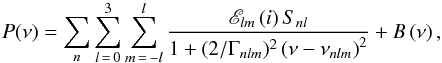 (1)where ν is the frequency, and B(ν) is the background noise. Here the sums are over the radial orders (typically ~8 values of n), the angular degrees l ≤ 3 and the azimuthal orders − l ≤ m ≤ l. Not all radial orders show clear l = 3 modes, and so only a few l = 3 modes are included in the fits, depending on the star. The mode power in a multiplet, Snl, is a free parameter. The mode visibility Elm(i) is a function of the inclination angle i of the rotation axis relative to the line of sight (see Gizon & Solanki 2003). We assume here that all modes share the same value of i.
The frequencies νnlm of the modes reveal the rotation information. For Sun-like stars rotating no more than a few times the solar rotation rate the mode frequencies can be parametrized as νnlm ≈ νnl + mδν, where δν is the rotational splitting. In our model fit we assume that the stellar interior rotates as a solid body, so that all modes share a common rotational splitting.
The full widths Γnlm = Γ(νnlm) of the Lorentzian profiles depend on the mode lifetimes, which in turn depend on the mode frequencies νnlm. In the Sun this variation with frequency can be modeled by a low-order polynomial (Stahn 2010). We therefore opt to parametrize the mode widths as a third-order polynomial in (ν − νmax), where νmax is the frequency at maximum power of the p-mode envelope. Note that only the l = 0 modes contribute to the fit of this function since they are not broadened or split by rotation.
The background noise level  is caused by several terms: the very long-term variability (hours to days) from magnetic activity, the variability (tens of minutes) from stellar surface granulation, and the photon noise. For asteroseismology applications, these noise components can be adequately described by two Harvey-like background terms (e.g., Handberg & Campante 2011) and a constant term to account for the white photon noise.
We find the best fit with maximum likelihood estimation using a Markov chain Monte Carlo sampler (Foreman-Mackey et al. 2013). The best-fit values of each parameter are estimated by the median of the corresponding marginalized posterior distribution, and the 16th and 84th percentile values of the distributions represent the errors. We fit the entire spectrum, including all mode parameters and background terms simultaneously (a so-called global fit), in contrast to Nielsen et al. (2014) who fit the background and separate sets of p-modes individually. A comparison between the global rotational splitting obtained in this work, and the mean of the rotational splittings measured by Nielsen et al. (2014) are shown in Table 1.
An example spectrum of KIC005184732 is shown in Fig. 1. The background terms dominate the low frequency end of the spectrum, while the p-mode envelope appears clearly above the noise level at ~1800 μHz. The inset shows a part of the p-mode envelope, where the splitting of an l = 2 mode is clearly visible.
2.2. Surface variability periods
The rotation of stars can also be inferred from the periodic variability of their light curves caused by surface features on the stellar disk, such as active regions. For the Sun, active regions are good tracers of the surface rotation of the plasma, to within a few percent (Beck 2000). In other stars this difference could potentially be larger.
From the periodic variation of the stellar light curve it is relatively straightforward to identify the rotation period of the star, and this has been done using automated routines for tens of thousands of stars (Nielsen et al. 2013; Reinhold & Reiners 2013; McQuillan et al. 2014). However, these routines typically rely on coherent surface variability over long time periods. The stars studied here do not show simple and regular surface variability and, therefore, they do not appear in these catalogs. Furthermore, the PDC_MAP pipeline (Smith et al. 2012; Stumpe et al. 2014) is known to suppress variability on timescales longer than ~20 days (Christiansen et al. 2013).
We therefore manually reduce the raw pixel data for each star, and search this and the PDC_MAP reduced data for signs of rotational variability. To reduce the raw data, we use the kepcotrend procedure in the PyKe software package2. The PyKe software uses a series of so-called cotrending basis vectors (CBVs) in an attempt to remove instrumental variability from the raw light curves. The CBVs are computed based on variability common to a large sample of stars on the detector, and so in principle represent the systematic variability. The number of CBVs to use in the reduction is not clear and we therefore compute several sets of reduced light curves using a sequentially increasing number of CBVs (up to six) for each star. We require that the variability appears in light curves reduced with different numbers of CBVs. This minimizes the risk of variability signatures that are caused by the reduction.
To measure the rotation period of each star we used the method of Nielsen et al. (2013). We compute the Lomb-Scargle periodogram (Lomb 1976; Scargle 1982) of each quarter and identify the peak of maximum power for periods less than 45 days. The median period of these peaks is used as a first order estimate of the rotation period. We then assume that active regions appear at similar latitudes, and so should have similar periods. This is done by requiring that peaks must lie within 4 median absolute deviations (MAD) from the median. The median and MAD of the remaining peak periods are the measured rotation period and error on the rotation period. Examples are shown in Fig. 2. The rotation periods of these stars measured using this method agree with those found by García et al. (2014)do Nascimento et al. (2014).
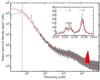 |
Fig. 1 Power density spectrum of the short cadence white light photometry time series of KIC005184732. Gray represents the spectrum smoothed with a 0.1 μHz wide Gaussian kernel, with the best-fit model shown in red. Black dashed indicates the surface variability frequency. The inset shows a zoom of the p-mode envelope at an l = 2,0 pair, where the black markers indicate the individual m-components. The separation between components of the l = 2 mode is the rotational splitting. |
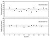 |
Fig. 2 Peak periods in the Lomb-Scargle periodogram as a function of observation quarter for KIC004914923 (top) and KIC005184732 (bottom). Solid gray shows the median period, and dashed gray shows the median absolute deviation. |
3. Comparing asteroseismic and surface variability periods
In Table 1 we list the periods for each analysis. These values are also shown in Fig. 3. The asteroseismic and surface variability periods agree very well for all the stars analyzed here. However, the asteroseismic rotation period measurements are systematically lower than those from surface variability. As a first order significance estimate of this difference we fit a linear function PS = aPA to the measured values. We find the best fit by maximum likelihood estimation, using the marginalized posterior distributions for the asteroseismic measurements, and assume Gaussian posterior distributions for the surface variability periods. The best-fit solution returns  , showing that the difference between the two measurement methods is insignificant (see Fig. 3). As a consistency check we perform an identical fit to the average rotation periods PN from Nielsen et al. (2014), assuming Gaussian errors (see Table 1). We find a slope of
  , in good agreement with the slope of PA. However, this does not account for the non-Gaussian form of the marginalized posteriors of the fits performed in that work.
 |
Fig. 3 Surface variability period PS as a function of asteroseismic period PA. The 1:1 line is shown with a black dashed line. The best-fit value and errors to the slope are shown with red solid and dashed lines, respectively. For comparison the Carrington period of 27.3 days is also shown (this is not included in the fit). |
4. Gyrochronology
Here we estimate the stellar ages from three different gyrochronology relations provided by Mamajek & Hillenbrand (2008), Barnes (2010), and García et al. (2014). These relations represent distinct methods of estimating gyrochronology ages. In all these relations, we use the asteroseismic rotation periods from Sect. 2.1.
The type of gyro-relation used by Mamajek & Hillenbrand (2008), first proposed by Barnes (2007), assumes that the rotation period of a star varies as powers of age and mass, where the B − V color is used as a proxy for the latter. This relation is calibrated to young cluster stars with ages ≲625 Gyr, with only the Sun representing the older stellar populations. For the stars studied here we use B − V values from Høg et al. (2000), using extinction values from the KIC catalog (Brown et al. 2011).
The relation by García et al. (2014) is calibrated to stars with asteroseismically determined ages from Mathur et al. (2012) and Metcalfe et al. (2014). However, this relation does not include a mass dependence since the calibrators are all similar in mass (~1 M⊙), and so this relation only depends on the rotation period of the star.
Lastly, the relation by Barnes (2010) incorporates the effects of a rapid spin-down phase, experienced by very young stars (~100 Myr), into the prediction of the stellar age. This relation uses convective turnover time τ as a proxy for mass, and is also calibrated using young cluster stars, with the Sun as the only anchoring point for older stars.
We determine the convective turnover times from stellar models fit to the stellar oscillation frequencies (see online material in Nielsen et al. 2014). These stellar models are produced using the Modules for Experiments in Stellar Astrophysics (MESA, Paxton et al. 2011, 2013), with the same input physics as in Ball & Gizon (2014). Initial fits were determined using the SEEK method (Quirion et al. 2010) to compare a grid of models to observed spectroscopic and global asteroseismic parameters. The models cover the mass range 0.60–1.60 M⊙ and initial metal abundances Z in the range 0.001–0.040. The helium abundance was presumed to follow the enrichment law Y = 0.245 + 1.45Z and the mixing length parameter was fixed at α⊙ = 1.908.
As initial guesses, we used the median values of the grid-based fit and also generated ten random, uniformly-distributed realizations of the parameters. The 11 initial guesses were optimized in five parameters (age, mass, metallicity, helium abundance, and mixing length) using a downhill simplex (Nelder & Mead 1965) to match spectroscopic data (Bruntt et al. 2012) and individual oscillation frequencies, computed with ADIPLS (Christensen-Dalsgaard 2008) and corrected according to the cubic correction by Ball & Gizon (2014). As in Ball & Gizon (2014), the seismic and nonseismic observations are weighted only by their respective measurement uncertainties. Best-fit parameters and uncertainties are estimated from ellipses bounding surfaces of constant χ2 for all the models determined during the optimizations, corresponding to a total of about 3000 models for each star.
The best-fit models yield local convective velocities and we use these to compute τ as in Kim & Demarque (1996), these are listed in Table 1. From these values of τ and the asteroseismic rotation periods from Sect. 2.1, we compute the gyrochronology ages using Eq. (32) from Barnes (2010) and the suggested calibration values therein.
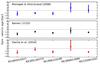 |
Fig. 4 Differences between gyrochronology ages and asteroseismic ages for three different gyrochronology relations. The relations are Mamajek & Hillenbrand (2008), Barnes (2010), and García et al. (2014). |
In addition to providing values of τ, the stellar models also produce estimates of the stellar ages. In Fig. 4 these ages are compared with those derived from the three gyrochronology relations. It is immediately obvious that the gyro-relations are in general not consistent with the seismic ages. For some stars a particular gyro-relation may agree well with the seismic age, but for other stars that same relation deviates significantly, as seen, e.g., for the ages from García et al. (2014) and Mamajek & Hillenbrand (2008) relations for KIC005184732 and KIC010963065. However, it appears that the gyro-relations tend to underestimate the stellar ages relative to the seismic values.
For the star KIC006933963, the gyro-relations predict an age older than the stellar models, which is likely because this star is a subgiant, with a slightly contracted core and expanded envelope. Thus, by angular momentum conservation one expects the surface and near-surface regions to have slowed down faster than the gyro-relations predict, leading to an overestimated age. KIC004914923 also appears to be a subgiant based on its core hydrogen content (see Table 1), but close inspection of the best-fit stellar model shows that this star has only just moved off the main sequence, and so may still adhere to these gyro-relations.
It should be noted that the errors on the asteroseismic ages are internal errors from the fit. However, even conservatively assuming a precision of ~20% on the asteroseismic ages (Aerts 2015), the two methods of age estimation are still in poor agreement.
5. Conclusions
We measured the rotation periods of five Sun-like stars, using asteroseismology and surface variability. The measurements show that the asteroseismic rotation periods are ~4% lower than those from surface variability, but this was not found to be a statistically significant difference given the measurement uncertainties. Thus there is no evidence for any radial (or latitudinal) differential rotation between the regions that the two methods are sensitive to.
Previous efforts to calibrate gyrochronology relations have focused on measuring rotation from surface variability of cluster stars. Given that rotation periods can be reliably determined by asteroseismology compared to the surface variability, gyrochronology may also be applied to very inactive stars for which surface variability rotation periods are not available.
Our comparison of three different gyrochronology relations from the literature found that these ages differed by up to several Gyr from the seismic ages. In general, the gyro-relations seemed to underestimate the stellar ages relative to the asteroseismic ages. It also demonstrated that the gyro-relations are not internally consistent.
When considering these discrepancies it is important to remember the calibrations used for each method. The Barnes (2010) and Mamajek & Hillenbrand (2008) relations are both calibrated using ages and rotation periods of the Sun and cluster stars, and so may not accurately predict ages of stars similar to or older than the Sun (e.g., Meibom et al. 2015). On the other hand, asteroseismic ages from stellar models are only calibrated to the Sun, and in addition are dependent on the input physics and assumptions of the stellar models (Lebreton & Goupil 2014). The relation by García et al. (2014) lacks a mass dependent term, in contrast to the two other tested relations. However, this was not expected to have a remarkable effect since the stars in our sample were approximately 1 M⊙ stars, similar to the calibrators used by García et al. (2014). Despite this, there is still a discrepancy of several Gyr between the ages derived from this relation and our seismic ages for some of the stars.
Tighter asteroseismic constraints for stellar modeling will become available when calibrations are obtained from cluster stars to be observed by space missions like K2 (Chaplin et al. 2015) and the Planetary Transits and Oscillations of stars (PLATO) mission (Rauer et al. 2014). This in turn will allow us to reliably use asteroseismic rotation periods to further refine gyrochronology relations for magnetically inactive field stars.
Downloaded from the Mikulski Archive for Space Telescopes, http://archive.stsci.edu/kepler/
Acknowledgments
The authors acknowledge research funding by Deutsche Forschungsgemeinschaft (DFG) under grant SFB 963/1 “Astrophysical flow instabilities and turbulence” (Project A18). L.G. acknowledges support from the Center for Space Science at NYU Abu Dhabi Institute under grant 73-71210-ADHPG-G1502. This paper includes data collected by the Kepler mission. Funding for the Kepler mission is provided by the NASA Science Mission directorate. Data presented in this paper were obtained from the Mikulski Archive for Space Telescopes (MAST). STScI is operated by the Association of Universities for Research in Astronomy, Inc., under NASA contract NAS5-26555. Support for MAST for non-HST data is provided by the NASA Office of Space Science via grant NNX09AF08G and by other grants and contracts.
References
- Aerts, C. 2015, Astron. Nachr., 336, 477 [NASA ADS] [CrossRef] [Google Scholar]
- Aerts, C., Thoul, A., Daszyńska, J., et al. 2003, Science, 300, 1926 [NASA ADS] [CrossRef] [PubMed] [Google Scholar]
- Ball, W. H., & Gizon, L. 2014, A&A, 568, A123 [NASA ADS] [CrossRef] [EDP Sciences] [Google Scholar]
- Barnes, S. A. 2007, ApJ, 669, 1167 [NASA ADS] [CrossRef] [Google Scholar]
- Barnes, S. A. 2010, ApJ, 722, 222 [NASA ADS] [CrossRef] [Google Scholar]
- Beck, J. G. 2000, Sol. Phys., 191, 47 [NASA ADS] [CrossRef] [Google Scholar]
- Borucki, W. J., Koch, D., Basri, G., et al. 2010, Science, 327, 977 [NASA ADS] [CrossRef] [PubMed] [Google Scholar]
- Brown, T. M., Latham, D. W., Everett, M. E., & Esquerdo, G. A. 2011, AJ, 142, 112 [NASA ADS] [CrossRef] [Google Scholar]
- Bruntt, H., Basu, S., Smalley, B., et al. 2012, MNRAS, 423, 122 [NASA ADS] [CrossRef] [Google Scholar]
- Chaplin, W. J., Bedding, T. R., Bonanno, A., et al. 2011, ApJ, 732, L5 [Google Scholar]
- Chaplin, W. J., Lund, M. N., Handberg, R., et al. 2015, PASP, accepted [arXiv:1507.01827] [Google Scholar]
- Charpinet, S., Fontaine, G., & Brassard, P. 2009, Nature, 461, 501 [NASA ADS] [CrossRef] [PubMed] [Google Scholar]
- Christensen-Dalsgaard, J. 2008, Ap&SS, 316, 113 [NASA ADS] [CrossRef] [Google Scholar]
- Christiansen, J. L., Jenkins, J. M., Caldwell, D. A., et al. 2013, Kepler Data Characteristics Handbook (KSCI – 19040 – 004) [Google Scholar]
- Davies, G. R., Chaplin, W. J., Farr, W. M., et al. 2015, MNRAS, 446, 2959 [NASA ADS] [CrossRef] [Google Scholar]
- do Nascimento, Jr., J.-D., García, R. A., Mathur, S., et al. 2014, ApJ, 790, L23 [NASA ADS] [CrossRef] [Google Scholar]
- D’Silva, S., & Howard, R. F. 1994, Sol. Phys., 151, 213 [NASA ADS] [CrossRef] [Google Scholar]
- Foreman-Mackey, D., Hogg, D. W., Lang, D., & Goodman, J. 2013, PASP, 125, 306 [CrossRef] [Google Scholar]
- García, R. A., Ceillier, T., Salabert, D., et al. 2014, A&A, 572, A34 [NASA ADS] [CrossRef] [EDP Sciences] [Google Scholar]
- Gizon, L., & Solanki, S. K. 2003, ApJ, 589, 1009 [NASA ADS] [CrossRef] [Google Scholar]
- Gizon, L., Ballot, J., Michel, E., et al. 2013, PNAS, 110, 13267 [NASA ADS] [CrossRef] [Google Scholar]
- Handberg, R., & Campante, T. L. 2011, A&A, 527, A56 [NASA ADS] [CrossRef] [EDP Sciences] [Google Scholar]
- Høg, E., Fabricius, C., Makarov, V. V., et al. 2000, A&A, 355, L27 [NASA ADS] [Google Scholar]
- Kim, Y.-C., & Demarque, P. 1996, ApJ, 457, 340 [NASA ADS] [CrossRef] [Google Scholar]
- Kurtz, D. W., Saio, H., Takata, M., et al. 2014, MNRAS, 444, 102 [NASA ADS] [CrossRef] [Google Scholar]
- Lebreton, Y., & Goupil, M. J. 2014, A&A, 569, A21 [NASA ADS] [CrossRef] [EDP Sciences] [Google Scholar]
- Lomb, N. 1976, Astrophys. Space Sci., 39, 447 [Google Scholar]
- Lund, M. N., Miesch, M. S., & Christensen-Dalsgaard, J. 2014, ApJ, 790, 121 [NASA ADS] [CrossRef] [Google Scholar]
- Mamajek, E. E., & Hillenbrand, L. A. 2008, ApJ, 687, 1264 [NASA ADS] [CrossRef] [Google Scholar]
- Mathur, S., Metcalfe, T. S., Woitaszek, M., et al. 2012, ApJ, 749, 152 [NASA ADS] [CrossRef] [Google Scholar]
- McQuillan, A., Mazeh, T., & Aigrain, S. 2014, ApJS, 211, 24 [NASA ADS] [CrossRef] [MathSciNet] [Google Scholar]
- Meibom, S., Barnes, S. A., Platais, I., et al. 2015, Nature, 517, 589 [NASA ADS] [CrossRef] [PubMed] [Google Scholar]
- Metcalfe, T. S., Creevey, O. L., Doğan, G., et al. 2014, ApJS, 214, 27 [NASA ADS] [CrossRef] [Google Scholar]
- Nelder, J. A., & Mead, R. 1965, The Computer Journal, 7, 308 [CrossRef] [Google Scholar]
- Nielsen, M. B., Gizon, L., Schunker, H., & Karoff, C. 2013, A&A, 557, L10 [NASA ADS] [CrossRef] [EDP Sciences] [Google Scholar]
- Nielsen, M. B., Gizon, L., Schunker, H., & Schou, J. 2014, A&A, 568, L12 [NASA ADS] [CrossRef] [EDP Sciences] [Google Scholar]
- Paxton, B., Bildsten, L., Dotter, A., et al. 2011, ApJS, 192, 3 [Google Scholar]
- Paxton, B., Cantiello, M., Arras, P., et al. 2013, ApJS, 208, 4 [NASA ADS] [CrossRef] [Google Scholar]
- Quirion, P.-O., Christensen-Dalsgaard, J., & Arentoft, T. 2010, ApJ, 725, 2176 [NASA ADS] [CrossRef] [Google Scholar]
- Rauer, H., Catala, C., Aerts, C., et al. 2014, Exp. Astron., 38, 249 [NASA ADS] [CrossRef] [Google Scholar]
- Reinhold, T., & Reiners, A. 2013, A&A, 557, A11 [NASA ADS] [CrossRef] [EDP Sciences] [Google Scholar]
- Scargle, J. D. 1982, ApJ, 283, 835 [NASA ADS] [CrossRef] [Google Scholar]
- Schou, J., Antia, H. M., Basu, S., et al. 1998, ApJ, 505, 390 [NASA ADS] [CrossRef] [Google Scholar]
- Skumanich, A. 1972, ApJ, 171, 565 [NASA ADS] [CrossRef] [Google Scholar]
- Smith, J. C., Stumpe, M. C., Van Cleve, J. E., et al. 2012, PASP, 124, 1000 [NASA ADS] [CrossRef] [Google Scholar]
- Snodgrass, H. B., & Ulrich, R. K. 1990, ApJ, 351, 309 [Google Scholar]
- Stahn, T. 2010, Ph.D. thesis, Göttingen University, Germany [Google Scholar]
- Stumpe, M. C., Smith, J. C., Catanzarite, J. H., et al. 2014, PASP, 126, 100 [NASA ADS] [CrossRef] [Google Scholar]
All Tables
All Figures
|
Fig. 1 Power density spectrum of the short cadence white light photometry time series of KIC005184732. Gray represents the spectrum smoothed with a 0.1 μHz wide Gaussian kernel, with the best-fit model shown in red. Black dashed indicates the surface variability frequency. The inset shows a zoom of the p-mode envelope at an l = 2,0 pair, where the black markers indicate the individual m-components. The separation between components of the l = 2 mode is the rotational splitting. |
| In the text | |
|
Fig. 2 Peak periods in the Lomb-Scargle periodogram as a function of observation quarter for KIC004914923 (top) and KIC005184732 (bottom). Solid gray shows the median period, and dashed gray shows the median absolute deviation. |
| In the text | |
|
Fig. 3 Surface variability period PS as a function of asteroseismic period PA. The 1:1 line is shown with a black dashed line. The best-fit value and errors to the slope are shown with red solid and dashed lines, respectively. For comparison the Carrington period of 27.3 days is also shown (this is not included in the fit). |
| In the text | |
|
Fig. 4 Differences between gyrochronology ages and asteroseismic ages for three different gyrochronology relations. The relations are Mamajek & Hillenbrand (2008), Barnes (2010), and García et al. (2014). |
| In the text | |
Current usage metrics show cumulative count of Article Views (full-text article views including HTML views, PDF and ePub downloads, according to the available data) and Abstracts Views on Vision4Press platform.
Data correspond to usage on the plateform after 2015. The current usage metrics is available 48-96 hours after online publication and is updated daily on week days.
Initial download of the metrics may take a while.