| Issue |
A&A
Volume 582, October 2015
|
|
|---|---|---|
| Article Number | A59 | |
| Number of page(s) | 90 | |
| Section | Interstellar and circumstellar matter | |
| DOI | https://doi.org/10.1051/0004-6361/201425190 | |
| Published online | 07 October 2015 | |
The large- and small-scale Ca II K structure of the Milky Way from observations of Galactic and Magellanic sightlines⋆,⋆⋆
1
European Southern Observatory,
Alonso de Cordova 3107, Vitacura,
Santiago,
Chile
e-mail:
This email address is being protected from spambots. You need JavaScript enabled to view it.
2
Astrophysics Research Centre, School of Mathematics and Physics,
Queen’s University Belfast, Belfast, BT7
1NN, UK
3
Space Telescope Science Institute, 3700 San Martin Drive, Baltimore, MD
21218,
USA
Received: 20 October 2014
Accepted: 18 June 2015
Abstract
Aims. The large and small-scale (pc) structure of the Galactic interstellar medium can be investigated by utilising spectra of early-type stellar probes of known distances in the same region of the sky. This paper determines the variation in line strength of Ca ii at 3933.661 Å as a function of probe separation for a large sample of stars, including a number of sightlines in the Magellanic Clouds.
Methods. FLAMES-GIRAFFE data taken with the Very Large Telescope towards early-type stars in 3 Galactic and 4 Magellanic open clusters in Ca ii are used to obtain the velocity, equivalent width, column density, and line width of interstellar Galactic calcium for a total of 657 stars, of which 443 are Magellanic Cloud sightlines. In each cluster there are between 43 and 111 stars observed. Additionally, FEROS and UVES Ca ii K and Na i D spectra of 21 Galactic and 154 Magellanic early-type stars are presented and combined with data from the literature to study the calcium column density – parallax relationship.
Results. For the four Magellanic clusters studied with FLAMES, the strength of the Galactic interstellar Ca ii K equivalent width on transverse scales from ~0.05−9 pc is found to vary by factors of ~1.8−3.0, corresponding to column density variations of ~0.3−0.5 dex in the optically-thin approximation. Using FLAMES, FEROS, and UVES archive spectra, the minimum and maximum reduced equivalent widths for Milky Way gas are found to lie in the range ~35−125 mÅ and ~30−160 mÅ for Ca ii K and Na i D, respectively. The range is consistent with a previously published simple model of the interstellar medium consisting of spherical cloudlets of filling factor ~0.3, although other geometries are not ruled out. Finally, the derived functional form for parallax (π) and Ca ii column density (NCaII) is found to be π(mas) = 1 / (2.39 × 10⁻¹³ × NCaII (cm-2) + 0.11). Our derived parallax is ~25 per cent lower than predicted by Megier et al. (2009, A&A, 507, 833) at a distance of ~100 pc and ~15 percent lower at a distance of ~200 pc, reflecting inhomogeneity in the Ca ii distribution in the different sightlines studied.
Key words: ISM: lines and bands / Galaxy: abundances / Magellanic Clouds / stars: early-type
Reduced spectra and Tables A.1−A.17 are only available at the CDS via anonymous ftp to cdsarc.u-strasbg.fr (130.79.128.5) or via http://cdsarc.u-strasbg.fr/viz-bin/qcat?J/A+A/582/A59
Figures A.1–A.37 are available in electronic form at http://www.aanda.org
Based on observations taken from the ESO archive, programme IDs 078.C-0493(A) and 171.D-0237(A).
© ESO, 2015
1. Introduction
Since its discovery in the interstellar medium more than 100 yr ago (Hartmann 1904), the Ca ii K line has been extensively studied. At 3933 Å it lies in a region of the spectrum that is free of strong telluric features and where CCD detectors are sensitive. Perhaps most importantly the transition itself is strong and hence easily detected in most high- resolution stellar spectra of medium signal-to-noise ratio (S/N). Recent studies of Ca ii include those by Albert et al. (1993), Sembach et al. (1993), Welty et al. (1996; at very high spectral resolution to obtain detailed information on cloud velocity components), Wakker & Mathis (2000; to determine the spread in the Ca/H ratio as a function of H i column density), and Smoker et al. (2003; to determine the Galactic scale-height of the transition). More recently, Megier et al. (2005; 2009) have compared the strength of the Ca ii K interstellar absorption with distances from the Hipparcos catalogue (ESA 1997) and open cluster distances to determine whether the line strength can be used to estimate distances to faraway objects. They found several cases of significant column density difference in the interstellar component of stars in the same cluster or association, but were unable to determine whether this was caused by a local contribution to the derived profiles, or by background or foreground stars being misclassified as cluster objects. Similar results were obtained by Smoker et al. (2011a,b), who observed three open clusters with UVES and found, within the same cluster, variations in interstellar column density in Ca ii and Na i D of up to ~0.5 and 1 dex, respectively. Authors such as Bowen et al. (1991), Kennedy et al. (1998), Meyer & Lauroesch (1999), Andrews et al. (2001), Smoker et al. (2003; 2011a,b), van Loon et al. (2009; 2013), Welsh et al. (2009), and Nasoudi-Shoar et al. (2010) attempted to eliminate the confusion by observing the centre of globular clusters, active galactic nuclei, or stars at high Galactic latitude in order to obtain the reduced Ca ii or Na i equivalent width. The current paper builds on some previous work by observing a total of 657 stars within seven open clusters, of which 443 objects lie in the Large and Small Magellanic Clouds. By comparison with many previous studies, smaller scales (~12 arcsec to 27 arcmin corresponding to ~0.05 to 15 pc) are studied, corresponding to the fieldsize of FLAMES1 which is ~30 arcmin, but still at a reasonable spectral resolution (~16 km s-1).
In addition to the small-scale FLAMES observations, the large-scale structure of the Milky Way is studied using FEROS2 and UVES3 via the observation in Ca ii K and Na i D of 154 stars in the Magellanic Clouds and 21 within the Galaxy at a resolution of ~4−8 km s-1. Our aim is to determine if current models of the interstellar medium (ISM) match the observations.
Section 2 describes the sample of open clusters and field stars, plus the data reduction and analysis performed to estimate the equivalent width and column density in the Galactic component in Ca ii and/or Na i D of the sightlines studied. In Sect. 3 we give the main results, including figures showing the interstellar profiles of the sightlines studied, as well as tables of the component fit parameters. Section 4 contains the discussion, in particular, focusing on the large- and small-scale variation observed in the Ca ii K and Na i D profiles towards the target stars and how variation in the former affects the use of the former species as a distance indicator. Using the FEROS and UVES Galactic sightlines plus archive data we determine the parallax – column density relationship for Ca ii and other lines and compare with the distance derived using spectroscopic parallax. Finally, Sect. 5 contains the summary and suggestions for future work. In what follows we define low velocity gas as having absolute values of velocity less than ~35 km s-1, intermediate- velocity gas with ~35 <v< ~90 km s-1, and high velocity gas with absolute velocities greater than ~90 km s-1.
2. The sample, data reduction, and analysis
The data on which the current paper is based were extracted from the ESO archive and are FLAMES-GIRAFFE observations towards three open clusters located in the Milky Way, and two in each of the Large and Small Magellanic Clouds, plus FEROS and UVES observations towards stars located in the Magellanic system and Milky Way.
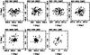 |
Fig. 1 FLAMES-GIRAFFE sample: Galactic coordinates of the sightlines for which low-velocity interstellar Ca ii K was detected. |
2.1. FLAMES-GIRAFFE archive sample towards open clusters in the MW and Magellanic System
The FLAMES data for the seven open clusters were taken from the ESO archive. Data reduction was performed using the ESO FLAMES pipeline within gasgano (Izzo et al. 2004) using calibrations taken on the day following the observation. For some observations the simultaneous calibration fibre was used. The HR2 grating was employed and measurements from a few spectra with the simultaneous calibration fibre enabled shows that the wavelength range was from ~3850 to 4045 Å with a spectral resolution around Ca ii K of R = λ/ Δλ ~ 18 500 or ~16 km s-1. The re-binned data from the pipeline were imported into IRAF4 where they were co-added using median addition within scombine and then read into dipso (Howarth et al. 1996). Subsequently, the spectra were normalised by fitting the continuum in regions bereft of interstellar features, and the S/N measured. At this stage a small number of late-type stars were excluded from the sample as in these cases distinguishing stellar from interstellar lines was problematical. For the early-type stars the stellar features were normally broad (cf. Mooney et al. 2002, 2004) and hence easily removed in the normalisation process. Table 1 shows basic data on the open clusters for which FLAMES data were analysed. Columns 1−5 give the cluster name, alternative name, location (Galactic or Magellanic), Galactic coordinates of the plate centre, and distance in kpc. Columns 6–8 give the total exposure time in seconds, median S/N per pixel around Ca ii K, and the number of stars used in the analysis. This number only includes objects where the Galactic interstellar component was useful and varies from 43 usable spectra for NGC 6611 to 111 for NGC 330, or a total of 657 sightlines with Ca ii interstellar measurements. Finally, Cols. 9−10 give the range of Galactic scales probed with the current measurements, being the minimum or maximum star-star separation at the distance of the cluster. For the Magellanic objects we assumed the scale height of the Galaxy in Ca ii K is ~800 pc (Smoker et al. 2003). Figure 1 shows the (l,b) coordinates of the stars used for each of the clusters. Tables A.1 to A.7 show the coordinates and magnitudes of the individual stars on which the FLAMES-MEDUSA fibres were placed.
Open cluster basic data observed with FLAMES sorted in terms of increasing NGC number.
2.2. FEROS and UVES archive data towards the Magellanic system
FEROS and UVES spectra of stars within the Large and Small Magellanic Clouds from several observing runs were also extracted from the ESO archive.
They are typically observations towards bright early-type O- and B- type stars. The Na i D observations are sometimes affected by Na in emission, although this always appears slightly offset from the Galactic absorption and was not fitted when performing profile fits. Telluric correction around the Na i D lines was performed by removing a scaled model of the sky smoothed to the spectral resolution of the observations using skycalc5.
The aim of extracting these spectra was to determine the variation in the Ca ii and Na i D Galactic column density on large scales. Authors such as Megier et al. (2009) found large variations in the Ca ii K line strength in Galactic open clusters, although could not rule out non-cluster contamination by background and foreground stars. The current observations of Magellanic targets eliminate the distance uncertainty and have median S/N of ~35 and ~80 per pixel in Ca ii and Na i, respectively. Table A.8 lists details of the 154 Magellanic Cloud targets observed. They are plotted in Fig. 2 and probe structures of size ≈5 deg, and hence act as a useful comparison to FLAMES observations of LMC and SMC targets in Sect. 2.1 that probe scales of less than ~30 arcmin.
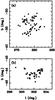 |
Fig. 2 Positions on the sky of stars taken from the FEROS and UVES archives used to investigate the large-scale structure variation of interstellar Galactic Ca ii K and Na i D. a) LMC sample; b) SMC sample. |
2.3. FEROS archive data towards Galactic early-type stars
Data towards Milky Way early-type stars from two observing runs were extracted from the FEROS archive. They are typically observations towards bright early-type O- and B- type stars. Authors such as Struve (1928), Megier et al. (2005; 2009) and references therein, have postulated the use of the Ca ii K line strength as a distance indicator for objects close to the Galactic plane. Table A.8 lists details of the Milky Way targets observed, with Fig. 3 showing their sky positions. The median S/N was ~200 and ~230 in Ca ii and Na i D, respectively. In Sect. 4.6 these observations are used with archive data to investigate the parallax – column density relationship for Ca ii K.
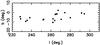 |
Fig. 3 Positions on the sky of data taken from the FEROS archive used to investigate the large-scale structure variation of Galactic Ca ii K and Na i D and the relationship between parallax and Ca ii column density. |
2.4. Data analysis; component fitting
For the Galactic absorption, interstellar components were fitted using both Gaussian fitting using the elf routine within the dipso software package, and also full profile Voigt-profile fitting using vapid (Howarth et al. 2002).
Simultaneous fitting was used for the Ca ii H and K line profiles within the whole sample, and for Na i D1 and D2 in the FEROS and UVES datasets. The Ca ii H line lies in the wing of Hϵ, and was hence normalised to provide a profile which could be fitted simultaneously with Ca ii K. Examples of Ca ii H and K spectra are shown in Fig. A.1.
ELF gives velocity centroids, full width half maxima and equivalent widths of the interstellar components. In addition, vapid yields estimates of the b-values and column densities of the profiles. The wavelength for Ca ii of 3933.661 Å and f-value of 0.627 were taken from Morton et al. (2003; 2004); conversion from Topocentric to the Local Standard of Rest (LSR) reference frame was performed using rv (Wallace & Clayton 1996). We note that due to the spectral resolution of the FLAMES-GIRAFFE data (~16 km s-1) it is likely that the interstellar profiles observed are in fact a superposition of many different components. For example, observations of Galactic gas in Ca ii K by Welty et al. (1996) show that the vast majority of components in their sample have b-values of between 0.5−3.0 km s-1, components that would be unresolved in the current dataset. In total Galactic interstellar profiles towards 657 stars were fitted. Smoker et al. (2015) separately describe the analysis of intermediate- and high-velocity clouds observed in the spectra towards the Magellanic Cloud targets.
Errors in the interstellar components were estimated using procedures outlined in Hunter et al. (2006). Briefly, these involve changing the column density and b-value of each component in turn until the residual in the model-data exceeds 1σ in 3 adjacent velocity bins. For the cases where no residual was above the limit even when the change equaled the measurement value, the error was set to the value of the measurement. This most frequently happened in the components with small b-values.
Two of the FEROS sample stars (HD 53244 and HD 76728) have very strong stellar lines around Ca ii and Na i hence profile fitting was not performed for these objects.
3. Results
In this section we present the reduced spectra and model fits for the FLAMES-GIRAFFE and FEROS/UVES sample.
3.1. FLAMES-GIRAFFE spectra
Figures A.2 to A.8 show the Ca ii K spectra towards each of the stars in the sample as well as the model fit obtained using Gaussian (ELF) fitting and the (data-model) residual fit. In order to assess the variations in the profiles, Figs. A.9 to A.15 show the 16 star-star pairs in each cluster with the largest differences in equivalent width, with no star being plotted more than once. Tables A.9 to A.15 show the corresponding Voigt profile fit results for each of the seven clusters studied.
3.2. FEROS and UVES spectra
Figure A.16 shows the FEROS and UVES Ca ii K, Na i D and corresponding GASS and LABS Survey 21-cm H i (Kalberla et al. 2005; McClure-Griffiths et al. 2009) spectra towards the 154 Magellanic Cloud and 21 Milky Way stars. The latter data have velocity resolution of ~1 km s-1, brightness temperature sensitivity of 0.06−0.07 K and spatial resolution of ~0.5° (LAB) and 16 arcmin (GASS). Tables A.16 and A.17 show the corresponding profile fits and total column densities derived from the optical data, plus the total derived H i Galactic column density derived from the equation; 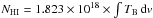 , where TB is the detected brightness temperature and dv is in km s-1.
Figures A.17 and A.18 show the 16 Magellanic sightlines pairs in Ca ii K and Na i D for which there is the greatest difference in column density. Each sightline is only plotted once.
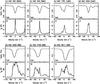 |
Fig. 4 Top panels: composite Ca ii K spectra towards each of the 7 clusters, formed by median combining the individual fibres after continuum normalisation. Bottom panels: 21-cm H i data taken from the GASS (full lines) and LABS survey (dotted lines) towards the FLAMES plate centres. a) NGC 330 (S/N~ 500; b) NGC 346 (S/N~ 900; c) NGC 1761 (S/N~ 1200; d) NGC 2004 (S/N~ 1000); e) NGC 3293 (S/N~ 800); f) NGC 4755 (S/N~ 800; g) NGC 6611 (S/N~ 500). Absorption-line features at ~ 50 km s-1 are caused by IV gas. |
4. Discussion
In this section we discuss the composite Ca ii K spectra and their comparison with single-dish H i 21-cm observations, the reduced equivalent widths and column densities for the local Ca ii gas as a function of sky position, the variation in the equivalent width with sky position and the velocity structure, the Ca/H i and Na/H i ratios as a function of N(H i), the Ca ii/Na i ratio, and finally the parallax – Ca ii column density relationship.
4.1. Composite GIRAFFE Ca II K spectra and comparison with 21-cm H I observations
Figure 4 shows the composite Ca ii K spectra towards each of the seven clusters, formed by median-combining the individual normalised spectra, weighting by the square of the S/N, and boxcar smoothing using a box of 3 pixels. We note that the FWHM of the arc lines is 4 pixels, so no degradation in resolution occurs due to the smoothing. The composite spectra have S/N ranging from ~500−1200, and display between 1−2 main components with velocities from –35 to +35 km s-1. Also shown in Fig. 4 are 21-cm H i data taken from the LABS and GASS surveys. Tables 2 and 3 show the results of component fitting to the composite Ca ii K and single-dish H i spectra, with values of the abundance A = log (N(Ca) /N(H i)) given. Although the ATCA-Parkes H i survey (Kim et al. 2003) of the Magellanic Clouds covers the LMC, no velocity information is available for the Galactic component.
For the three Galactic clusters the H i in emission has significantly more velocity structure than the Ca ii in absorption, which is simply a reflection of the difference in path lengths studied, with the clusters being at distances of ~2-kpc compared with the extent of the Milky Way disc in H i that extends beyond a radius of 40-kpc (e.g. Kalberla et al. 2007 and references therein). For three of the four Magellanic clusters, the main low-velocity peaks observed in the H i spectra are also visible in the Ca ii data. The exception is NGC 2004 for which there are two bright H i components separated by ~8 km s-1 plus an IV component at +40 km s-1 but for which only one Ca ii component is detected at a spectral resolution of ~16 km s-1. This Ca ii feature has a FWHM (corrected for instrumental broadening) of ~27 km s-1, indicative of two or more components (otherwise the kinetic temperature of the gas would be extremely high).
We comment finally on the NGC 1761 interstellar spectra in H i and Ca ii K. In H i there is a weak emission feature at ~−20 km s-1 and another much stronger one at ~3 km s-1. The component at −20 km s-1 has a [Ca ii/H i] equivalent width/column density ratio approximately 4 times larger than that at +3 km s-1. This increasing ratio with velocity is frequently seen and is generally thought to be caused by calcium being liberated from dust into the gas phase in intermediate- and high-velocity gas (e.g. Wakker & Matthis 2000).
Ca ii ELF fit results for the composite FLAMES-GIRAFFE spectra.
H i fit results for the LABS spectrum at the coordinate of the centre of the FLAMES-GIRAFFE pointing for the Magellanic objects.
4.2. Reduced equivalent widths and column densities for Ca II K and Na I D and comparison with previous work
Figure A.19 shows the point-to-point variation in total column density and percentage difference in equivalent width as a function of transverse separation for each of the 7 clusters observed with FLAMES. The column densities and equivalent widths were integrated between the velocity limits shown on the figures in order to exclude intermediate-, high- and Magellanic Cloud velocity components. We again note that due to the relatively low spectral resolution of the FLAMES-GIRAFFE dataset, unresolved components are likely to be present that make the column densities very uncertain.
Bowen et al. (1991) and Smoker et al. (2003) find reduced equivalent width (REW) values in the Ca ii K line for objects at infinity of ~110 mÅ (with 95 percent of lines lying between 60−310 mÅ) and 113 mÅ, respectively, where the REW is defined as EW × sin(b). In the current FLAMES-GIRAFFE dataset for the 4 Magellanic clusters in Ca ii K we find REW values for Galactic gas ranging from ~35−125 mÅ (see Table 4), with median values of ~40–70 mÅ on scales of ~0.05–6 pc. For the individual stars observed by FEROS and UVES, the corresponding range is ~30–125 mÅ in Ca ii K and ~50–155 mÅ in Na i D, with median values of 45 and 100 mÅ, respectively. Figure 5 shows histogrammes of the REW for low-velocity gas observed in absorption towards four Magellanic clusters, with Fig. 6 showing the corresponding histogrammes for the Galactic clusters. For the MC sightlines the reduced equivalent widths are approximately half the values of those observed in previous work (Bowen et al. 1991), and again indicate large-scale variations in the EW of optical absorption lines.
For the FLAMES-GIRAFFE sightlines, the maximum variation in REW in low-velocity gas over the ~5 pc field of view is a factor 3.0 for NGC 330 (which has lower S/N than the other sightlines), 1.8 for NGC 346, 1.8 for NGC 1761 and 1.6 for NGC 2004. These variations are somewhat smaller than observed in the intermediate-velocity and high-velocity gas towards the same sightlines, where the Ca ii K REW for example towards NGC 2004 varies by factors exceeding 10 (Smoker et al. 2015). Of course, the IV gas is likely to be at larger distances than the LV gas, hence the transverse scales sampled are bigger. Previous studies of small-scale (~0.03 pc) structure using binaries or the cores of globular clusters (e.g. Meyer & Blades 1996; Lauroesch & Meyer 1999; Lauroesch 2007 and references therein) have found strong variations in Na i D profiles on small scales, but much smaller changes in Ca ii K equivalent widths or column densities. The current observations confirm that such equivalent width variations in Ca ii also exist on scales of ~0.05–6 pc, with variation of ~0.3–0.5 dex in the optically thin approximation.
Figure 7 shows histograms of the reduced equivalent width and reduced column density for the two FEROS/UVES-observed species. For the LMC-only sightlines, 68 percent of the Ca ii reduced column densities lie within ±0.16 dex of log[N(Ca ii cm-2)] = 11.85. For the Na i data, 68 percent of the reduced column densities lie within ±0.32 dex of log[N(Na i cm-2)] = 11.93, reflecting the generally higher clumpiness of this neutral species compared with Ca ii. Finally, Fig. 8 shows the sightlines that display the biggest and smallest reduced equivalent width values for the low velocity gas in Ca ii K and Na i D for the Magellanic Cloud targets.
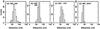 |
Fig. 5 Panels a)–d) Histogrammes of reduced equivalent width in the Ca ii K interstellar line for Magellanic open clusters NGC 330, NGC 346, NGC 1761 and NGC 2004. The integration limits are the same as in Fig. A.19. |
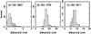 |
Fig. 6 Panels a)–c) Histogrammes of reduced equivalent width in the Ca ii K interstellar line for Milky Way clusters NGC 3293, NGC 4755, NGC 6611. The integration limits are the same as in Fig. A.19. |
Reduced equivalent width values for Galactic (low-velocity) gas using stellar probes.
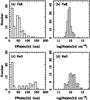 |
Fig. 7 Histogrammes of reduced equivalent width (REW) (panels a) and c)), and reduced column density (panels b) and d)) for Ca ii K and Na i D data from the Magellanic FEROS and UVES sample for gas with LSR velocities between –35 and +35 km s-1. Note that a number of targets do not have REW measurements due to the presence of stellar lines. See Table 9 for details. |
For over fifty years astronomers have thought that hierarchical structures and turbulence exist in the ISM (von Weizsacker 1951; von Hoerner 1951; see reviews by Elmegreen & Scalo 2004; Dickey 2007; Hennebelle & Falgarone 2012; and Falceta-Goncalves et al. 2014). The power spectrum of the ISM has often been used to provide coarse-scale information on structures present in the ISM and indicate how much material is present at each scale. However, it provides little information about the shape of the structures themselves, i.e. very different structures can produce similar power spectra (Chappell & Scalo 2001). In any case, with the incompletely-sampled FLAMES and FEROS data we cannot obtain a reliable power spectrum of the column density variations. Hence we restrict ourselves to a comparison between our work and the similar observational and theoretical study of Van Loon et al. (2009). Their observations towards ω Cen found that the real fluctuations in the column density maps on scales of half a degree were seven per cent in Ca ii (1 standard deviation). The fluctuations detected in Ca ii K are shown in Table 4 for our seven clusters. In the case of the Magellanic clusters, the 1σ variation in equivalent width for the FLAMES-observed field-of-view ranges from nine to 15 per cent (for NGC 330 and NGC 346, respectively) for Ca ii in the gas phase with velocities between –35 and +35 km s-1. For the three Galactic clusters the variation is 63 percent (NGC 3293), ten per cent (NGC 4755) and 15 per cent for NGC 6611. These are upper limits, not taking the errors on the measurements into account. For the FEROS/UVES spectra which span tens of degrees on the plane of the sky, the variation in column density is unsurprisingly much larger, being ~51 per cent in Ca ii.
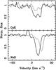 |
Fig. 8 FEROS and UVES spectra. Top panel: Ca ii spectra of Magellanic targets for the sightlines that have largest and smallest reduced equivalent widths between –35 and +35 km s-1. One star is from the SMC and one from the LMC although we are probing Galactic gas. Bottom panel: Corresponding data for the same two stars for Na i D. Filled lines: LHA 115-S 23 (SMC). Dotted lines: SK –67 256 (LMC). |
Van Loon et al. (2009) presented a simple model of the ISM as a collection of spherical cloudlets with filling factor 0.3 and sizes between 1 AU and 10 pc (their Appendix B). The model predicts observed fluctuations in the column density of the ISM on scales of 0.5 deg of 0.1–0.2, consistent with our observed values. However, other physical forms of the ISM such as sheets or filaments may also be consistent with the observed variations (e.g. Heiles 1997; Gómez & Vázquez-Semadeni 2014 and refs. therein). Indeed, Herschel observations of molecular clouds have detected a wealth of filaments towards the Gould Belt, with typical widths of around 0.1 pc (André et al. 2010), although to our knowledge there are no existing optical absorption line data that show filaments of such size in the warm ISM.
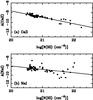 |
Fig. 9 A vs. N(H i) for FEROS and UVES Magellanic sightlines for gas with LSR velocities between –35 and +35 km s-1. The full lines are from Wakker & Mathis (2000) a) Ca ii K. b) Na i D. |
4.3. Variation in the Galactic velocity centroid and component structure
Figures A.20 to A.26 show the velocity centroid of the main Galactic Ca ii K component for each of the clusters observed with FLAMES-GIRAFFE. There are hints of gradients in the velocity centroid for this low-velocity component in the GIRAFFE data only towards NGC 1761 (north to south in Galactic coordinates with a magnitude of a few km s-1), and towards NGC 2004 (north-west to south-east of a few km s-1 over a 0.5 deg field). These probe Galactic gas with maximum transverse scales of ~5 pc. Figures A.27 and A.28 show the corresponding plots for the LV gas for the Magellanic stars observed with FEROS. The SMC clusters NGC 330 and NGC 346 are generally well fitted by only one component at low velocities, although in particular for NGC 330 there are sometimes indications of two-component structure that would need a better S/N and/or spectral resolution to resolve. Considering the LMC clusters, for NGC 1761 there are generally two strong low-velocity components, and one for NGC 2004 (although both frequently show intermediate- and high-velocity gas, discussed in Smoker et al. 2015). For the Galactic clusters, NGC 3293 can often be fit with a single component (e.g. Star 2372 in Fig. A.6), although the residuals in other sightlines (e.g. Star 2341) imply another component may be needed, and in yet other sightlines (e.g. Star 2303) there is clearly more than one component. Nevertheless, the overall shape of the Ca ii K profile is similar in all sightlines. More variation in profile shape is apparent towards Galactic cluster NGC 4755, with all sightlines needing two or three components to be well-fitted. Finally, towards NGC 6611 there is also a large variation in the two to four interstellar components present.
4.4. Ca II/H I and Na I/H I ratios in the Galactic ISM from observations of stars in the Magellanic Clouds
Values of the estimated Galactic Ca ii and Na i abundances A were derived from log(Nopt)/log(NHI) (where Nopt is the column density of either Ca ii or Na i). Figures 9a and b show the corresponding fits of A against NHI for Ca ii and Na i respectively, with the best-fitting lines from Wakker & Mathis (2000) overlaid. We note that Wakker & Mathis only plotted data up to log[N(H i cm-2)] ~ 21.4, and that for the current dataset ionisation effects have not been taken into account. Neither has H2 nor the large difference in resolution between the optical and H i observations. For both Ca ii and Na i, at column densities smaller than log[N(H i)] = 21.4, the values of A lie within the 1σ scatter of 0.42 and 0.52 dex, respectively, given in Wakker & Mathis (2000). However, at higher H i column densities the extrapolation of the best fit of Wakker & Mathis (2000) lies ~1 dex above the observed A values for Ca ii. Also, the scatter in A for Na i markedly increases at high values of H i. This may be caused in part by saturation effects, and ideally the current sightlines should be re-observed in Na i at 3303 Å to eliminate this possibility.
4.5. The Ca II/Na I ratio in the FEROS/UVES Magellanic sightlines
For LV gas the [Ca ii/Na i] ratio ranges from ~–0.9 to +0.6 dex which is within the range of ~–1 to 100 derived for example by Siluk & Silk (1974) and Vallerga et al. (1993). The Ca ii/Na i column density ratio is a common diagnostic of the ISM (Hobbs 1975; Welty et al. 1999; van Loon et al. 2009; Welsh et al. 2009 amongst others), due to the fact that Ca shows a large range in depletion, depending on the temperature and presence of dust (e.g. Bertin et al. 1993). Welty et al. (1999) note that if Ca ii is the dominant species, then the ratio [Ca ii/Na i] depends primarily on the Ca depletion and the temperature. In warm gas (T ~ 3000 K), Ca i is enhanced and Ca iii can also be a major contributor to the total Ca column density (Sembach et al. 2000). Figure 10 shows this ratio plotted against Ca ii K column density for the FEROS and UVES Magellanic sightlines alone. A weak trend in increasing [Ca ii/Na i] with Ca ii K column density is present, although this could be in part explained by saturation issues. A future paper will look at these and other data in more detail to investigate the [Ca ii/Na i] ratio as a function of velocity (the Routly-Spitzer effect; Routly & Spitzer 1952; Vallerga et al. 1993).
Figure 11 shows the FEROS and UVES-observed [Ca ii/Na i] ratio for low-velocity gas, derived using Magellanic objects, as a function of H i column density for LV gas as obtained from the LABS survey. There is an anti-correlation between the two quantities, explained by the fact that the neutral species Na i and H i both probe cooler parts of the ISM than Ca ii which tends to be depleted onto dust as the H i column density increases.
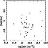 |
Fig. 10 [Ca ii K/Na i D] ratio plotted against log[Ca ii K] for low velocity gas for the FEROS and UVES Magellanic sightlines alone. |
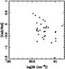 |
Fig. 11 [Ca ii K/Na i D] ratio plotted against log[H i] for low velocity gas for the FEROS and UVES Magellanic sightlines alone. |
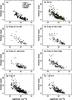 |
Fig. 12 a) Hipparcos parallax against log N(Ca ii K) for stars in the current Galactic FEROS sample plus objects taken from the literature. The red line is the best-fit from Megier et al. (2009). The green line is the best fit derived from the current data to the function π = 1 / (A × N + b) where A = 2.39 × 10⁻¹³ and b = 0.11. b)–h) Corresponding plots with data taken from the compilation of Gudennavar et al. (2012) and a range of Galactic latitude and longitudes. |
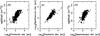 |
Fig. 13 a) Log(Ca ii cm-2) against Log(paralactic distance pc). b) Log(Spectroscopic parallax distance pc) against Log(paralactic distance pc) c) Log(Ca ii cm-2) against Log(Spectroscopic parallax distance pc). Parallaxes and spectral types are from simbad. Only stars of spectral type V are included in the plot. Ca ii column densities are taken from Gudennavar et al. (2012). |
4.6. The parallax – column density correlation for Ca II and other species
Authors including Beals & Oke (1953), Megier et al. (2005; 2009) and Welsh et al. (2010) find a slowly-increasing Ca ii equivalent width with increasing distance, although with a large scatter. At distances greatly exceeding 100 pc, Welsh et al. (1997) note that the increase in column density is more associated with the number of clouds sampled along a particular sight-line as opposed to the actual distance. Figure 12a shows the Hipparcos parallax plotted against the log of the Ca ii K column density for all the objects in the current paper for which both quantities are available. Additionally, we have used results from Sembach et al. (1993); Hunter et al. (2006) and Smoker et al. (2011a,b) to produce a sample of 125 sightlines with parallaxes ranging from ~11 mas down to zero. Superimposed on the plot is the best-fit line from Megier et al. (2009) which has the form π = 1 / (2.29 × 10⁻¹³ × NCaII + 0.77) (n = 262), where NCaII is in cm-2. At small distances (large values of parallax), the equation from Megier et al. predicts larger parallaxes at a given log(NCaII) than observed in our present dataset, ranging from a ~25 per cent difference at 100 pc distance, to ~15 per cent at 200 pc. This is likely just a reflection of the differing sightlines used in the two datasets, as previously observed when results from Megier et al. (2005) and Megier et al. (2009) are compared. We note that the Local Bubble has dimensions of around ~100 pc (e.g. Breitschwerdt et al. 1998; Welsh & Shelton 2009 and references therein), and hence the column densities in this region are frequently very low (e.g. Frisch & York 1983). Therefore, any analytical formula for the parallax/column density is likely to fail in this regime. The best fit that we obtain is;  (1)which is also displayed on the figure. To further evaluate the relationship, we have plotted in Figs. 12b−h the parallaxes against Ca ii column densities taken from the compilation of Gudennavar et al. (2012), the most extensive dataset of such measurements available in the literature. In particular, Fig. 12b shows 419 data points with absolute values of Galactic latitude less than 10.0°, with the best-fit lines from Megier et al. (2009) and the current result superimposed. Figures A.29 to A.37 shows the corresponding plot of parallax against column density for the 38 species from Gudennavar et al. (2012). Clear correlations (although with large scatters) are visible in Al i (few data points), Ca ii, D i (few data points), Mn ii, Na i, O vi, P ii and Ti ii. Of these, only Mn ii and P ii are typically the dominant ionisation stage in the warm ISM (Sembach et al. 2000). Hence it is likely that other factors, such as dust depletion and inherant clumpiness of the element, causes much of the observed scatter. In particular, S ii is both the dominant ionisation stage and typically the element is thought to be little depleted onto dust grains in the diffuse ISM. However, the parallax/column density relationship for this line shows no reduced scatter compared with other elements.
Finally, in Fig. 13 we plot the Hipparcos parallax against the Ca ii column density, the Hipparcos parallax against the spectroscopic parallax and the spectroscopic parallax against the Ca ii column density. Data are taken from Gudennavar et al. (2012) and we only include stars of spectral type V in the comparision. The spectroscopic parallaxes used absolute magnitudes and colours from Schmidt-Kaler (1982) and Wegner (1994), from which we estimated the reddening and hence the distance to the stars in question. Straight line fits between 100 pc and 1000 pc for CaII/Hipparcos, Spectroscopic/Hipparcos and CaII/Spectroscopic result in scatters in the ordinate of 0.67, 0.35 and 0.60, respectively. Hence between these distance limits the scatter in the parallax vs. spectroscopic parallax fit is 0.25 dex or a factor 1.8 smaller than the parallax vs. Ca ii column density fit. We have attempted to improve the correlation by only including sightlines where log(Ca ii/Na i) exceeds 0.5, to exclude instances with cooler gas present in which the Ca ii is locked up in dust grains. However, the correlation between parallax and Ca ii is not significantly improved when using this subsample.
5. Summary and suggestions for future work
We have described the use of FLAMES, FEROS, and UVES archive data towards field stars and open clusters in the Milky Way and Magellanic Clouds to obtain information on the variability of Ca ii in the Galactic interstellar medium and its possible use as a distance indicator. We find that towards four Magellanic open clusters the maximum variation observed is between a factor of ~1.8 and 3 in equivalent width or ~0.3−0.5 dex in column density in the optically thin approximation over fields of size ~0.05–6 pc. These observations can be explained by a simple model of the ISM presented in van Loon et al. (2009) although likely other functional forms of the ISM would also match the observations. Using archive observations and results from the literature we derive a parallax – column density relationship for Milky Way gas in Ca ii of π(mas) = 1/(2.39 × 10-13 × NCaII (cm-2 + 0.11) that predicts parallaxes to within 15 percent of the Megier et al. (2009) values for distances of 200 pc.
A future paper will use the FLAMES HR4 grating setting to study the variation in the Ca i and CH+ lines at 4226 Å and 4232 Å, respectively, for the sample of clusters discussed here, to determine the variation in neutral and molecular column density. New observations using the Na i D line could probe the variation in the Routley-Spitzer effect on small scales and how it changes with reddening.
Online material
Appendix A: Additional figures
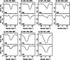 |
Fig. A.1 Example Ca ii H and K spectra towards the seven clusters observed with FLAMES-GIRAFFE. |
 |
Fig. A.2 FLAMES-GIRAFFE Ca ii K spectra towards NGC 330 in the SMC. Data are in the LSR and the spectral resolution is ~16 km s-1. |
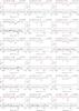 |
Fig. A.2 continued. NGC 330 Ca ii FLAMES-GIRAFFE spectra. |
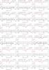 |
Fig. A.2 continued. NGC 330 Ca ii FLAMES-GIRAFFE spectra. |
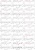 |
Fig. A.2 continued. NGC 330 Ca ii FLAMES-GIRAFFE spectra. |
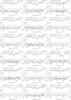 |
Fig. A.2 continued. NGC 330 Ca ii FLAMES-GIRAFFE spectra. |
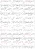 |
Fig. A.2 continued. NGC 330 Ca ii FLAMES-GIRAFFE spectra. |
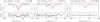 |
Fig. A.2 continued. NGC 330 Ca ii FLAMES-GIRAFFE spectra. |
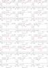 |
Fig. A.3 FLAMES-GIRAFFE Ca ii K spectra towards NGC 346 in the SMC. Data are in the LSR and the spectral resolution is ~16 km s-1. |
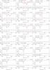 |
Fig. A.3 continued. NGC 346 Ca ii FLAMES-GIRAFFE spectra. |
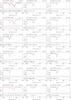 |
Fig. A.3 continued. NGC 346 Ca ii FLAMES-GIRAFFE spectra. |
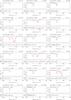 |
Fig. A.3 continued. NGC 346 Ca ii FLAMES-GIRAFFE spectra. |
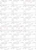 |
Fig. A.3 continued. NGC 346 Ca ii FLAMES-GIRAFFE spectra. |
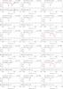 |
Fig. A.3 continued. NGC 346 Ca ii FLAMES-GIRAFFE spectra. |
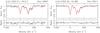 |
Fig. A.3 continued. NGC 346 Ca ii FLAMES-GIRAFFE spectra. |
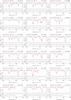 |
Fig. A.4 FLAMES-GIRAFFE Ca ii K spectra towards NGC 1761 (LH 09) in the LMC. Data are in the LSR and the spectral resolution is ~16 km s-1. |
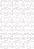 |
Fig. A.4 continued. NGC 1761 Ca ii FLAMES-GIRAFFE spectra. |
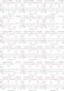 |
Fig. A.4 continued. NGC 1761 Ca ii FLAMES-GIRAFFE spectra. |
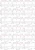 |
Fig. A.4 continued. NGC 1761 Ca ii FLAMES-GIRAFFE spectra. |
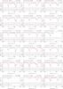 |
Fig. A.4 continued. NGC 1761 Ca ii FLAMES-GIRAFFE spectra. |
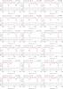 |
Fig. A.4 continued. NGC 1761 Ca ii FLAMES-GIRAFFE spectra. |
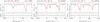 |
Fig. A.4 continued. NGC 1761 Ca ii FLAMES-GIRAFFE spectra. |
 |
Fig. A.5 FLAMES-GIRAFFE Ca ii K spectra towards NGC 2004 in the LMC. Data are in the LSR and the spectral resolution is ~16 km s-1. |
 |
Fig. A.5 continued. NGC 2004 Ca ii FLAMES-GIRAFFE spectra. |
 |
Fig. A.5 continued. NGC 2004 Ca ii FLAMES-GIRAFFE spectra. |
 |
Fig. A.5 continued. NGC 2004 Ca ii FLAMES-GIRAFFE spectra. |
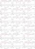 |
Fig. A.5 continued. NGC 2004 Ca ii FLAMES-GIRAFFE spectra. |
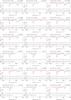 |
Fig. A.5 continued. NGC 2004 Ca ii FLAMES-GIRAFFE spectra. |
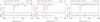 |
Fig. A.5 continued. NGC 2004 Ca ii FLAMES-GIRAFFE spectra. |
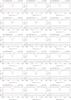 |
Fig. A.6 FLAMES-GIRAFFE Ca ii K spectra towards NGC 3293 in the Milky Way. Data are in the LSR and the spectral resolution is ~16 km s-1. |
 |
Fig. A.6 continued. NGC 3293 Ca ii FLAMES-GIRAFFE spectra. |
 |
Fig. A.6 continued. NGC 3293 Ca ii FLAMES-GIRAFFE spectra. |
 |
Fig. A.6 continued. NGC 3293 Ca ii FLAMES spectra. |
 |
Fig. A.6 continued. NGC 3293 Ca ii FLAMES spectra. |
 |
Fig. A.7 FLAMES-GIRAFFE Ca ii K spectra towards NGC 4755 in the Milky Way. Data are in the LSR and the spectral resolution is ~16 km s-1. |
 |
Fig. A.7 continued. NGC 4755 Ca ii FLAMES-GIRAFFE spectra. |
 |
Fig. A.7 continued. NGC 4755 Ca ii FLAMES-GIRAFFE spectra. |
 |
Fig. A.7 continued. NGC 4755 Ca ii FLAMES-GIRAFFE spectra. |
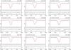 |
Fig. A.7 continued. NGC 4755 Ca ii FLAMES-GIRAFFE spectra. |
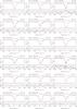 |
Fig. A.8 FLAMES-GIRAFFE Ca ii K spectra towards NGC 6611 in the Milky Way. Data are in the LSR and the spectral resolution is ~16 km s-1. |
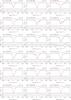 |
Fig. A.8 continued. NGC 6611 Ca ii FLAMES-GIRAFFE spectra. |
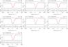 |
Fig. A.8 continued. NGC 6611 Ca ii FLAMES-GIRAFFE spectra. |
 |
Fig. A.9 Ca ii K spectra towards NGC 330 showing the spectra of 16 star-to-star pairs in which the maximum difference in the equivalent width was detected between a velocity of −35 and +35 km s-1 in the LSR. Each star is only plotted once. |
 |
Fig. A.10 Ca ii K spectra towards NGC 346 showing the spectra of 16 star-to-star pairs in which the maximum difference in the equivalent width was detected between a velocity of −35 and +35 km s-1 in the LSR. Each star is only plotted once. |
 |
Fig. A.11 Ca ii K spectra towards NGC 1761 showing the spectra of 16 star-to-star pairs in which the maximum difference in the equivalent width was detected between a velocity of −60 and +30 km s-1 in the LSR. Each star is only plotted once. |
 |
Fig. A.12 Ca ii K spectra towards NGC 2004 showing the spectra of 16 star-to-star pairs in which the maximum difference in the equivalent width was detected between a velocity of −35 and +35 km s-1 in the LSR. Each star is only plotted once. |
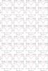 |
Fig. A.13 Ca ii K spectra towards NGC 3293 showing the spectra of 16 star-to-star pairs in which the maximum difference in the equivalent width was detected between a velocity of −80 and +60 km s-1 in the LSR. Each star is only plotted once. |
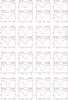 |
Fig. A.14 Ca ii K spectra towards NGC 4755 showing the spectra of 16 star-to-star pairs in which the maximum difference in the equivalent width was detected between a velocity of −80 and +60 km s-1 in the LSR. Each star is only plotted once. |
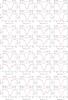 |
Fig. A.15 Ca ii K spectra towards NGC 6611 showing the spectra of 16 star-to-star pairs in which the maximum difference in the equivalent width was detected between a velocity of −80 and +100 km s-1 in the LSR. Each star is only plotted once. |
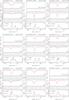 |
Fig. A.16 Top panels: FEROS or UVES Ca ii K (3933 Å) and Na i D1 (5889 Å) profiles towards Galactic and Magellenic stars, showing the observed spectrum in the LSR, Voigt model fit and data-model residual. Bottom panel: corresponding H i data from the GASS (black line) and LABS (dotted red line) surveys. |
 |
Fig. A.16 continued. FEROS or UVES Ca ii K, Na i D and GASS or LABS H i spectra. |
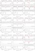 |
Fig. A.16 continued. FEROS or UVES Ca ii K, Na i D and GASS or LABS H i spectra. |
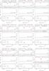 |
Fig. A.16 continued. FEROS or UVES Ca ii K, Na i D and GASS or LABS H i spectra. |
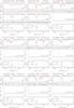 |
Fig. A.16 continued. FEROS or UVES Ca ii K, Na i D and GASS or LABS H i spectra. |
 |
Fig. A.16 continued. FEROS or UVES Ca ii K, Na i D and GASS or LABS H i spectra. |
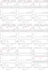 |
Fig. A.16 continued. FEROS or UVES Ca ii K, Na i D and GASS or LABS H i spectra. |
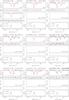 |
Fig. A.16 continued. FEROS or UVES Ca ii K, Na i D and GASS or LABS H i spectra. |
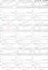 |
Fig. A.16 continued. FEROS or UVES Ca ii K, Na i D and GASS or LABS H i spectra. |
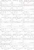 |
Fig. A.16 continued. FEROS or UVES Ca ii K, Na i D and GASS or LABS H i spectra. |
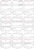 |
Fig. A.16 continued. FEROS or UVES Ca ii K, Na i D and GASS or LABS H i spectra. |
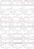 |
Fig. A.16 continued. FEROS or UVES Ca ii K, Na i D and GASS or LABS H i spectra. |
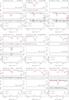 |
Fig. A.16 continued. FEROS or UVES Ca ii K, Na i D and GASS or LABS H i spectra. |
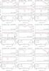 |
Fig. A.16 continued. FEROS or UVES Ca ii K, Na i D and GASS or LABS H i spectra. |
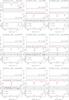 |
Fig. A.16 continued. FEROS or UVES Ca ii K, Na i D and GASS or LABS H i spectra. |
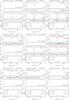 |
Fig. A.16 continued. FEROS or UVES Ca ii K, Na i D and GASS or LABS H i spectra. |
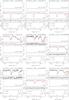 |
Fig. A.16 continued. FEROS or UVES Ca ii K, Na i D and GASS or LABS H i spectra. |
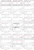 |
Fig. A.16 continued. FEROS or UVES Ca ii K, Na i D and GASS or LABS H i spectra. |
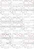 |
Fig. A.16 continued. FEROS or UVES Ca ii K, Na i D and GASS or LABS H i spectra. |
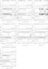 |
Fig. A.16 continued. FEROS or UVES Ca ii K, Na i D and GASS or LABS H i spectra. |
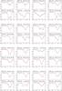 |
Fig. A.17 FEROS Ca ii K spectra towards the Magellanic clouds showing the spectra of 16 star-to-star pairs in which the maximum difference in the equivalent width was detected between a velocity of −35 and +35 km s-1 in the LSR. Each star is only plotted once. |
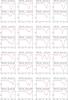 |
Fig. A.18 FEROS Na i D spectra towards the Magellanic clouds showing the spectra of 16 star-to-star pairs in which the maximum difference in the equivalent width was detected between a velocity of −35 and +35 km s-1 in the LSR. Each star is only plotted once. |
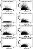 |
Fig. A.19 Left panels: variation in total Ca ii K column density between the limits in LSR km s-1 shown on the figures as a function of star-to-star sky separation in degrees as observed by FLAMES-GIRAFFE. Right panels: corresponding percentage variation in observed Ca ii K equivalent width. a), b): NGC 330, c), d): NGC 346, e), f): NGC 1761, g), h): NGC 2004. |
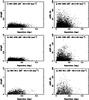 |
Fig. A.19 continued. i), j): NGC 3293, k), l): NGC 4755, m), n): NGC 6611. |
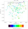 |
Fig. A.20 FLAMES-GIRAFFE NGC 330 (SMC) equivalent width and velocity map for low velocity gas where larger symbol sizes correspond to larger equivalent widths. Sightlines with uncorrected FWHM velocities greater than 20 km s-1 have been excluded from the plot. |
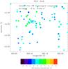 |
Fig. A.21 FLAMES-GIRAFFE NGC 346 (SMC) equivalent width and velocity map for low velocity gas where larger symbol sizes correspond to larger equivalent widths. Sightlines with uncorrected FWHM velocities greater than 20 km s-1 have been excluded from the plot. |
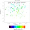 |
Fig. A.22 FLAMES-GIRAFFE NGC 1761 (LMC) equivalent width and velocity map for low velocity gas where larger symbol sizes correspond to larger equivalent widths. Sightlines with uncorrected FWHM velocities greater than 20 km s-1 have been excluded from the plot. |
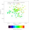 |
Fig. A.23 FLAMES-GIRAFFE NGC 2004 (LMC) equivalent width and velocity map for low velocity gas where larger symbol sizes correspond to larger equivalent widths. Sightlines with uncorrected FWHM velocities greater than 20 km s-1 have been excluded from the plot. |
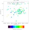 |
Fig. A.24 FLAMES-GIRAFFE NGC 3293 (Milky Way) equivalent width and velocity map for low velocity gas where larger symbol sizes correspond to larger equivalent widths. Sightlines with uncorrected FWHM velocities greater than 20 km s-1 have been excluded from the plot. |
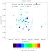 |
Fig. A.25 FLAMES-GIRAFFE NGC 4755 (LMC) equivalent width and velocity map for low velocity gas where larger symbol sizes correspond to larger equivalent widths. Sightlines with uncorrected FWHM velocities greater than 20 km s-1 have been excluded from the plot. |
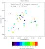 |
Fig. A.26 FLAMES-GIRAFFE NGC 6611 (LMC) equivalent width and velocity map for low velocity gas where larger symbol sizes correspond to larger equivalent widths. Sightlines with uncorrected FWHM velocities greater than 20 km s-1 have been excluded from the plot. |
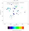 |
Fig. A.27 The Magellanic Clouds. Equivalent width and velocity map for Low-Velocity gas for Ca ii K where larger symbol sizes correspond to larger equivalent widths. Sightlines with uncorrected FWHM velocities greater than 20 km s-1 have been excluded from the plot. |
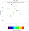 |
Fig. A.28 The Magellanic Clouds. Equivalent width and velocity map for Low-Velocity gas for Na i D where larger symbol sizes correspond to larger equivalent widths. Sightlines with uncorrected FWHM velocities greater than 20 km s-1 have been excluded from the plot. |
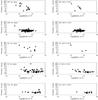 |
Fig. A.29 (a) Parallax vs. column density for Al ii, Al iii, Ar i, C i and C i* with the data being taken from Gudennavar et al. (2012). All available sightlines and sighlines with |b| < 10° are shown. |
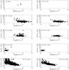 |
Fig. A.30 (b) Parallax vs. column density for Cl ii, C iv, C2, Ca i and Ca ii with the data being taken from Gudennavar et al. (2012). All available sightlines and sighlines with |b| < 10° are shown. |
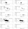 |
Fig. A.31 (c) Parallax vs. column density for Cu ii, D i, F i, Fe ii and Fe iii with the data being taken from Gudennavar et al. (2012). All available sightlines and sighlines with |b| < 10° are shown. |
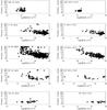 |
Fig. A.32 (d) Parallax vs. column density for Ge ii, H, H i, H2 and HD with the data being taken from Gudennavar et al. (2012). All available sightlines and sighlines with |b| < 10° are shown. |
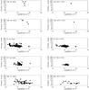 |
Fig. A.33 (e) Parallax vs. column density for He i, He ii, K .i, Kr i and Mg i with the data being taken from Gudennavar et al. (2012). All available sightlines and sighlines with |b| < 10° are shown. |
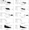 |
Fig. A.34 (f) Parallax vs. column density for Mg ii, Mn ii, N i, N ii and Na i with the data being taken from Gudennavar et al. (2012). All available sightlines and sighlines with |b| < 10° are shown. |
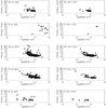 |
Fig. A.35 (g) Parallax vs. column density for Ni ii, O i, O vi, P ii, and S i with the data being taken from Gudennavar et al. (2012). All available sightlines and sighlines with |b| < 10° are shown. |
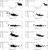 |
Fig. A.36 (h) Parallax vs. column density for S ii, Si ii, Si iv, Ti ii, Zn i and a combination of Ca ii, Mn ii and P ii with the data being taken from Gudennavar et al. (2012). All available sightlines and sighlines with |b| < 10° are shown. |
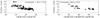 |
Fig. A.37 (i) Parallax vs. column density for a combination of a combination of Ca ii plus Ti ii and Ca ii, Mn ii and P ii with the data being taken from Gudennavar et al. (2012). All available sightlines and sighlines with |b| < 10° are shown. |
FLAMES (Pasquini et al. 2002) is a multi-object, intermediate- and high-resolution spectrograph, mounted at the VLT/Unit Telescope 2 (Kueyen) at Cerro Paranal, Chile, operated by ESO.
FEROS (Kaufer et al. 1999) is a high- resolution echelle spectrograph, mounted at the 2.2 m Telescope at La Silla, Chile, operated by ESO.
IRAF is distributed by the National Optical Astronomy Observatories, USA.
skycalc is available at https://www.eso.org/observing/etc/skycalc
Acknowledgments
This paper makes use of data taken from the Archive of the European Southern Observatory. This research has made use of the simbad database, operated at CDS, Strasbourg, France. J.V.S. thanks Queen’s University Belfast for financial support under the visiting scientist scheme and to ESO for financial support under the Director General’s Discressionary fund. We would like to thank an anonymous referee for their careful reading of the original manuscript.
References
- Albert, C. E., Blades, J. C., Morton, D. C., et al. 1993, ApJS, 88, 81 [NASA ADS] [CrossRef] [Google Scholar]
- André, Ph., Men’shchikov, A., Bontemps, S., et al. 2010, A&A, 518, A102 [Google Scholar]
- Andrews, S. M., Meyer, D. M., & Lauroesch, J. T. 2001, ApJ, 552, 73 [Google Scholar]
- Beals, C. S., & Oke, J. B. 1953, MNRAS, 113, 530 [NASA ADS] [CrossRef] [Google Scholar]
- Bertin, P., Lallement, R., Ferlet, R., & Vidal-Madjar, A. 1993, A&A, 278, 549 [NASA ADS] [Google Scholar]
- Bowen, D. V. 1991, MNRAS, 251, 649 [NASA ADS] [Google Scholar]
- Breitschwerdt, D., Freyberg, M., & Truemper, J. 1998, in The local bubble and beyond, LNP (Berlin: Springer), IAU Coloq., 166, 506 [Google Scholar]
- Chappell, D., & Scalo, J. 2001, MNRAS, 325, 1 [NASA ADS] [CrossRef] [Google Scholar]
- Dekker, H., D’Odorico, S., Kaufer, A., Delabre, B., & Kotzlowski, H. 2000, SPIE, 4008, 534 [Google Scholar]
- Dickey, J. M. 2007, IAU Symp., 237, 1 [NASA ADS] [Google Scholar]
- Elmegreen, B. G., & Scalo, J. 2004, ARA&A, 42, 211 [NASA ADS] [CrossRef] [Google Scholar]
- ESA 1997, The Hipparcos and Tycho Catalogues (Noordwijk: ESA), ESA SP 1200 [Google Scholar]
- Falceta-Goncalves, D., Kowal, G., Falgarone, E., & Chian, A. C.-L. 2014, Nonlin. Processes Geophys., 21, 587 [CrossRef] [Google Scholar]
- Frisch, P. C., & York, D. G. 1983, ApJ, 271, 59 [NASA ADS] [CrossRef] [Google Scholar]
- Gómez Gilberto, C., & Vázquez-Semadeni, E. 2014, ApJ, 791, 124 [NASA ADS] [CrossRef] [Google Scholar]
- Gudennavar, S. B., Bubbly, S. G., Preethi, K., & Murthy, J. 2012, ApJS, 199, 8 [NASA ADS] [CrossRef] [Google Scholar]
- Hartmann, J. 1904, ApJ, 19, 268 [Google Scholar]
- Heiles, C. 1997, ApJ, 481, 193 [NASA ADS] [CrossRef] [Google Scholar]
- Hennebelle, P., & Falgarone, E. 2012, A&ARv, 20, 55 [NASA ADS] [CrossRef] [Google Scholar]
- Hobbs, L. 1975, ApJ, 202, 628 [NASA ADS] [CrossRef] [Google Scholar]
- Howarth, I. D., Murray, J., Mills, D., & Berry, D. S. 1996, Starlink User Note SUN 50, Rutherford Appleton Laboratory/CCLRC [Google Scholar]
- Howarth, I. D., Price, R. J., Crawford, I. A., & Hawkins, I. 2002, 335, 267 [Google Scholar]
- Hunter, I., Smoker, J. V., Keenan, F. P., et al. 2006, MNRAS, 367, 1478 [CrossRef] [Google Scholar]
- Izzo, C., Kornweibel, N., McKay, D., et al. 2004, The Messenger, 117, 33 [NASA ADS] [Google Scholar]
- Kalberla, P. M. W., Burton, W. B., Hartmann, D., et al. 2005, A&A, 440, 775 [NASA ADS] [CrossRef] [EDP Sciences] [Google Scholar]
- Kalberla, P. M. W., Dedes, L., Kerp, J., & Haud, U. 2007, A&A, 469, 511 [NASA ADS] [CrossRef] [EDP Sciences] [Google Scholar]
- Kaufer, A., Stahl, O., Tubbesing, S., et al. 1999, The Messenger 95, 8 [Google Scholar]
- Keller, S. C., & Wood, P. R. 2006, ApJ, 642, 834 [NASA ADS] [CrossRef] [Google Scholar]
- Kennedy, D. C., Bates, B., & Kemp, S. N. 1998, A&A, 336, 315 [NASA ADS] [Google Scholar]
- Kim, S., Staveley-Smith, L., Dopita, M. A., et al. 2003, ApJS, 148, 473 [NASA ADS] [CrossRef] [Google Scholar]
- Lauroesch, J. T. 2007, SINS – Ionized and Neutral Structures in the diffuse interstellar medium, ASP Conf. Ser., 365, 40 [NASA ADS] [Google Scholar]
- Lauroesch, J. T., & Meyer, D. M. 1999, Apj, 519, 181 [Google Scholar]
- McClure-Griffiths, N. M., Pisano, D. J., Calabretta, M. R., et al. 2009, ApJS, 181, 398 [NASA ADS] [CrossRef] [Google Scholar]
- Megier, A., Strobel, A., Bondar, A., et al. 2005, ApJ, 634, 451 [NASA ADS] [CrossRef] [Google Scholar]
- Megier, A., Strobel, A., Galazutdinov, G. A., & Krelowski, J. 2009, A&A, 507, 833 [NASA ADS] [CrossRef] [EDP Sciences] [Google Scholar]
- Meyer, D. M., & Blades, J. C. 1996, ApJ, 464, 179 [Google Scholar]
- Meyer, D., & Lauroesch, J. T. 1999, ApJ, 520, 103 [Google Scholar]
- Mooney, C. J., Rolleston, W. R. J., Keenan, F. P., et al. 2002, MNRAS, 337, 851 [NASA ADS] [CrossRef] [Google Scholar]
- Mooney, C. J., Rolleston, W. R. J., Keenan, F. P., et al. 2004, A&A, 419, 1123 [NASA ADS] [CrossRef] [EDP Sciences] [Google Scholar]
- Morton, D. C. 2003, ApJS, 149, 205 [NASA ADS] [CrossRef] [MathSciNet] [Google Scholar]
- Morton, D. C. 2004, ApJS, 151, 403 [NASA ADS] [CrossRef] [Google Scholar]
- Nasoudi-Shoar, S., Richter, P., de Boer, K. S., & Wakker, B. P. 2010, A&A, 520, A26 [NASA ADS] [CrossRef] [EDP Sciences] [Google Scholar]
- Pasquini, L., Avila, G., Blecha, A., et al. 2002, The Messenger 110, 1 [Google Scholar]
- Routly, P. M., & Spitzer, L. 1952, ApJ, 115, 227 [NASA ADS] [CrossRef] [Google Scholar]
- Schmidt-Kaler, Th. 1982, in eds. K. Schaifers, & H. H. Voigt, Vol. 2, Landolt-Boernstein, group VI, subvol. b, Stars and Star Clusters (Berlin: Springer), 17 [Google Scholar]
- Sembach, K. R., Danks, A. C., & Savage, B. D. 1993, A&AS, 100, 107 [NASA ADS] [Google Scholar]
- Sembach, K. R., Howk, J. C., Ryans, R. S. I., & Keenan, F. P. 2000, ApJ, 528, 310 [NASA ADS] [CrossRef] [Google Scholar]
- Siluk, R. S., & Silk, J. 1974, ApJ, 192, 51 [NASA ADS] [CrossRef] [Google Scholar]
- Smoker, J. V., Rolleston, W. R. J., Kay, H. R. M., et al. 2003, MNRAS, 346, 119 [NASA ADS] [CrossRef] [Google Scholar]
- Smoker, J. V., Haddad, N., Iwert, O., et al. 2009, Msngr, 138, 8 [Google Scholar]
- Smoker, J. V., Fox, F. P., & Keenan, F. P. 2011a, MNRAS, 415, 1105 [NASA ADS] [CrossRef] [Google Scholar]
- Smoker, J. V., Bagnulo, S., Cabanac, R., et al. 2011b, MNRAS, 414, 59 [NASA ADS] [CrossRef] [Google Scholar]
- Smoker, J. V., Fox, A. J., & Keenan, F. P. 2015, MNRAS, 451, 4346 [NASA ADS] [CrossRef] [Google Scholar]
- Struve, O., Bailey, M., & Tatton, B. L. 1928, ApJ, 108, 242 [Google Scholar]
- Vallerga, J. V., Vedder, P. W., Craig, N., & Welsh, B. Y. 1993, ApJ, 411, 729 [NASA ADS] [CrossRef] [Google Scholar]
- von Hoerner, S. 1951, Astrophysik, 30, 17 [Google Scholar]
- van Loon, J. T., Smith, K. T., McDonald, I., et al. 2009, MNRAS, 399, 195 [NASA ADS] [CrossRef] [Google Scholar]
- van Loon, J. T., Bailey, M., Tatton, B. L., et al. 2013, A&A, 550, A108 [NASA ADS] [CrossRef] [EDP Sciences] [Google Scholar]
- von Weizsacker, C. F., 1951, ApJ, 114, 165 [NASA ADS] [CrossRef] [Google Scholar]
- Wakker, B. P., & Mathis, J. S. 2000, ApJ, 544, 107 [Google Scholar]
- Wallace, P., & Clayton, C 1996, rv, Starlink User Note SUN 78, Rutherford Appleton Laboratory/CCLRC [Google Scholar]
- Wegner, W. 1994, MNRAS, 270, 229 [NASA ADS] [CrossRef] [Google Scholar]
- Welsh, B. Y., & Shelton, R. L. 2009, ApSS, 323, 1 [Google Scholar]
- Welsh, B. Y., Sasseen, T., Craig, N., et al. 1997, ApJS, 112, 507 [NASA ADS] [CrossRef] [Google Scholar]
- Welsh, B. Y., Wheatley, J., & Lallement, R. 2009, PASP, 121, 606 [NASA ADS] [CrossRef] [Google Scholar]
- Welsh, B. Y., Lallement, R., Vergely, J.-L., & Raimond, S. 2010, A&A, 510, A54 [NASA ADS] [CrossRef] [EDP Sciences] [Google Scholar]
- Welty, D. E., Morton, D. C., & Hobbs, L. M. 1996, ApJS, 106, 533 [NASA ADS] [CrossRef] [Google Scholar]
- Welty, D. E., Frisch, P. C., Sonnerborn, G., & York, D. G. 1999, ApJ, 512, 636 [NASA ADS] [CrossRef] [Google Scholar]
All Tables
Open cluster basic data observed with FLAMES sorted in terms of increasing NGC number.
H i fit results for the LABS spectrum at the coordinate of the centre of the FLAMES-GIRAFFE pointing for the Magellanic objects.
Reduced equivalent width values for Galactic (low-velocity) gas using stellar probes.
All Figures
|
Fig. 1 FLAMES-GIRAFFE sample: Galactic coordinates of the sightlines for which low-velocity interstellar Ca ii K was detected. |
| In the text | |
|
Fig. 2 Positions on the sky of stars taken from the FEROS and UVES archives used to investigate the large-scale structure variation of interstellar Galactic Ca ii K and Na i D. a) LMC sample; b) SMC sample. |
| In the text | |
|
Fig. 3 Positions on the sky of data taken from the FEROS archive used to investigate the large-scale structure variation of Galactic Ca ii K and Na i D and the relationship between parallax and Ca ii column density. |
| In the text | |
|
Fig. 4 Top panels: composite Ca ii K spectra towards each of the 7 clusters, formed by median combining the individual fibres after continuum normalisation. Bottom panels: 21-cm H i data taken from the GASS (full lines) and LABS survey (dotted lines) towards the FLAMES plate centres. a) NGC 330 (S/N~ 500; b) NGC 346 (S/N~ 900; c) NGC 1761 (S/N~ 1200; d) NGC 2004 (S/N~ 1000); e) NGC 3293 (S/N~ 800); f) NGC 4755 (S/N~ 800; g) NGC 6611 (S/N~ 500). Absorption-line features at ~ 50 km s-1 are caused by IV gas. |
| In the text | |
|
Fig. 5 Panels a)–d) Histogrammes of reduced equivalent width in the Ca ii K interstellar line for Magellanic open clusters NGC 330, NGC 346, NGC 1761 and NGC 2004. The integration limits are the same as in Fig. A.19. |
| In the text | |
|
Fig. 6 Panels a)–c) Histogrammes of reduced equivalent width in the Ca ii K interstellar line for Milky Way clusters NGC 3293, NGC 4755, NGC 6611. The integration limits are the same as in Fig. A.19. |
| In the text | |
|
Fig. 7 Histogrammes of reduced equivalent width (REW) (panels a) and c)), and reduced column density (panels b) and d)) for Ca ii K and Na i D data from the Magellanic FEROS and UVES sample for gas with LSR velocities between –35 and +35 km s-1. Note that a number of targets do not have REW measurements due to the presence of stellar lines. See Table 9 for details. |
| In the text | |
|
Fig. 8 FEROS and UVES spectra. Top panel: Ca ii spectra of Magellanic targets for the sightlines that have largest and smallest reduced equivalent widths between –35 and +35 km s-1. One star is from the SMC and one from the LMC although we are probing Galactic gas. Bottom panel: Corresponding data for the same two stars for Na i D. Filled lines: LHA 115-S 23 (SMC). Dotted lines: SK –67 256 (LMC). |
| In the text | |
|
Fig. 9 A vs. N(H i) for FEROS and UVES Magellanic sightlines for gas with LSR velocities between –35 and +35 km s-1. The full lines are from Wakker & Mathis (2000) a) Ca ii K. b) Na i D. |
| In the text | |
|
Fig. 10 [Ca ii K/Na i D] ratio plotted against log[Ca ii K] for low velocity gas for the FEROS and UVES Magellanic sightlines alone. |
| In the text | |
|
Fig. 11 [Ca ii K/Na i D] ratio plotted against log[H i] for low velocity gas for the FEROS and UVES Magellanic sightlines alone. |
| In the text | |
|
Fig. 12 a) Hipparcos parallax against log N(Ca ii K) for stars in the current Galactic FEROS sample plus objects taken from the literature. The red line is the best-fit from Megier et al. (2009). The green line is the best fit derived from the current data to the function π = 1 / (A × N + b) where A = 2.39 × 10⁻¹³ and b = 0.11. b)–h) Corresponding plots with data taken from the compilation of Gudennavar et al. (2012) and a range of Galactic latitude and longitudes. |
| In the text | |
|
Fig. 13 a) Log(Ca ii cm-2) against Log(paralactic distance pc). b) Log(Spectroscopic parallax distance pc) against Log(paralactic distance pc) c) Log(Ca ii cm-2) against Log(Spectroscopic parallax distance pc). Parallaxes and spectral types are from simbad. Only stars of spectral type V are included in the plot. Ca ii column densities are taken from Gudennavar et al. (2012). |
| In the text | |
|
Fig. A.1 Example Ca ii H and K spectra towards the seven clusters observed with FLAMES-GIRAFFE. |
| In the text | |
|
Fig. A.2 FLAMES-GIRAFFE Ca ii K spectra towards NGC 330 in the SMC. Data are in the LSR and the spectral resolution is ~16 km s-1. |
| In the text | |
|
Fig. A.2 continued. NGC 330 Ca ii FLAMES-GIRAFFE spectra. |
| In the text | |
|
Fig. A.2 continued. NGC 330 Ca ii FLAMES-GIRAFFE spectra. |
| In the text | |
|
Fig. A.2 continued. NGC 330 Ca ii FLAMES-GIRAFFE spectra. |
| In the text | |
|
Fig. A.2 continued. NGC 330 Ca ii FLAMES-GIRAFFE spectra. |
| In the text | |
|
Fig. A.2 continued. NGC 330 Ca ii FLAMES-GIRAFFE spectra. |
| In the text | |
|
Fig. A.2 continued. NGC 330 Ca ii FLAMES-GIRAFFE spectra. |
| In the text | |
|
Fig. A.3 FLAMES-GIRAFFE Ca ii K spectra towards NGC 346 in the SMC. Data are in the LSR and the spectral resolution is ~16 km s-1. |
| In the text | |
|
Fig. A.3 continued. NGC 346 Ca ii FLAMES-GIRAFFE spectra. |
| In the text | |
|
Fig. A.3 continued. NGC 346 Ca ii FLAMES-GIRAFFE spectra. |
| In the text | |
|
Fig. A.3 continued. NGC 346 Ca ii FLAMES-GIRAFFE spectra. |
| In the text | |
|
Fig. A.3 continued. NGC 346 Ca ii FLAMES-GIRAFFE spectra. |
| In the text | |
|
Fig. A.3 continued. NGC 346 Ca ii FLAMES-GIRAFFE spectra. |
| In the text | |
|
Fig. A.3 continued. NGC 346 Ca ii FLAMES-GIRAFFE spectra. |
| In the text | |
|
Fig. A.4 FLAMES-GIRAFFE Ca ii K spectra towards NGC 1761 (LH 09) in the LMC. Data are in the LSR and the spectral resolution is ~16 km s-1. |
| In the text | |
|
Fig. A.4 continued. NGC 1761 Ca ii FLAMES-GIRAFFE spectra. |
| In the text | |
|
Fig. A.4 continued. NGC 1761 Ca ii FLAMES-GIRAFFE spectra. |
| In the text | |
|
Fig. A.4 continued. NGC 1761 Ca ii FLAMES-GIRAFFE spectra. |
| In the text | |
|
Fig. A.4 continued. NGC 1761 Ca ii FLAMES-GIRAFFE spectra. |
| In the text | |
|
Fig. A.4 continued. NGC 1761 Ca ii FLAMES-GIRAFFE spectra. |
| In the text | |
|
Fig. A.4 continued. NGC 1761 Ca ii FLAMES-GIRAFFE spectra. |
| In the text | |
|
Fig. A.5 FLAMES-GIRAFFE Ca ii K spectra towards NGC 2004 in the LMC. Data are in the LSR and the spectral resolution is ~16 km s-1. |
| In the text | |
|
Fig. A.5 continued. NGC 2004 Ca ii FLAMES-GIRAFFE spectra. |
| In the text | |
|
Fig. A.5 continued. NGC 2004 Ca ii FLAMES-GIRAFFE spectra. |
| In the text | |
|
Fig. A.5 continued. NGC 2004 Ca ii FLAMES-GIRAFFE spectra. |
| In the text | |
|
Fig. A.5 continued. NGC 2004 Ca ii FLAMES-GIRAFFE spectra. |
| In the text | |
|
Fig. A.5 continued. NGC 2004 Ca ii FLAMES-GIRAFFE spectra. |
| In the text | |
|
Fig. A.5 continued. NGC 2004 Ca ii FLAMES-GIRAFFE spectra. |
| In the text | |
|
Fig. A.6 FLAMES-GIRAFFE Ca ii K spectra towards NGC 3293 in the Milky Way. Data are in the LSR and the spectral resolution is ~16 km s-1. |
| In the text | |
|
Fig. A.6 continued. NGC 3293 Ca ii FLAMES-GIRAFFE spectra. |
| In the text | |
|
Fig. A.6 continued. NGC 3293 Ca ii FLAMES-GIRAFFE spectra. |
| In the text | |
|
Fig. A.6 continued. NGC 3293 Ca ii FLAMES spectra. |
| In the text | |
|
Fig. A.6 continued. NGC 3293 Ca ii FLAMES spectra. |
| In the text | |
|
Fig. A.7 FLAMES-GIRAFFE Ca ii K spectra towards NGC 4755 in the Milky Way. Data are in the LSR and the spectral resolution is ~16 km s-1. |
| In the text | |
|
Fig. A.7 continued. NGC 4755 Ca ii FLAMES-GIRAFFE spectra. |
| In the text | |
|
Fig. A.7 continued. NGC 4755 Ca ii FLAMES-GIRAFFE spectra. |
| In the text | |
|
Fig. A.7 continued. NGC 4755 Ca ii FLAMES-GIRAFFE spectra. |
| In the text | |
|
Fig. A.7 continued. NGC 4755 Ca ii FLAMES-GIRAFFE spectra. |
| In the text | |
|
Fig. A.8 FLAMES-GIRAFFE Ca ii K spectra towards NGC 6611 in the Milky Way. Data are in the LSR and the spectral resolution is ~16 km s-1. |
| In the text | |
|
Fig. A.8 continued. NGC 6611 Ca ii FLAMES-GIRAFFE spectra. |
| In the text | |
|
Fig. A.8 continued. NGC 6611 Ca ii FLAMES-GIRAFFE spectra. |
| In the text | |
|
Fig. A.9 Ca ii K spectra towards NGC 330 showing the spectra of 16 star-to-star pairs in which the maximum difference in the equivalent width was detected between a velocity of −35 and +35 km s-1 in the LSR. Each star is only plotted once. |
| In the text | |
|
Fig. A.10 Ca ii K spectra towards NGC 346 showing the spectra of 16 star-to-star pairs in which the maximum difference in the equivalent width was detected between a velocity of −35 and +35 km s-1 in the LSR. Each star is only plotted once. |
| In the text | |
|
Fig. A.11 Ca ii K spectra towards NGC 1761 showing the spectra of 16 star-to-star pairs in which the maximum difference in the equivalent width was detected between a velocity of −60 and +30 km s-1 in the LSR. Each star is only plotted once. |
| In the text | |
|
Fig. A.12 Ca ii K spectra towards NGC 2004 showing the spectra of 16 star-to-star pairs in which the maximum difference in the equivalent width was detected between a velocity of −35 and +35 km s-1 in the LSR. Each star is only plotted once. |
| In the text | |
|
Fig. A.13 Ca ii K spectra towards NGC 3293 showing the spectra of 16 star-to-star pairs in which the maximum difference in the equivalent width was detected between a velocity of −80 and +60 km s-1 in the LSR. Each star is only plotted once. |
| In the text | |
|
Fig. A.14 Ca ii K spectra towards NGC 4755 showing the spectra of 16 star-to-star pairs in which the maximum difference in the equivalent width was detected between a velocity of −80 and +60 km s-1 in the LSR. Each star is only plotted once. |
| In the text | |
|
Fig. A.15 Ca ii K spectra towards NGC 6611 showing the spectra of 16 star-to-star pairs in which the maximum difference in the equivalent width was detected between a velocity of −80 and +100 km s-1 in the LSR. Each star is only plotted once. |
| In the text | |
|
Fig. A.16 Top panels: FEROS or UVES Ca ii K (3933 Å) and Na i D1 (5889 Å) profiles towards Galactic and Magellenic stars, showing the observed spectrum in the LSR, Voigt model fit and data-model residual. Bottom panel: corresponding H i data from the GASS (black line) and LABS (dotted red line) surveys. |
| In the text | |
|
Fig. A.16 continued. FEROS or UVES Ca ii K, Na i D and GASS or LABS H i spectra. |
| In the text | |
|
Fig. A.16 continued. FEROS or UVES Ca ii K, Na i D and GASS or LABS H i spectra. |
| In the text | |
|
Fig. A.16 continued. FEROS or UVES Ca ii K, Na i D and GASS or LABS H i spectra. |
| In the text | |
|
Fig. A.16 continued. FEROS or UVES Ca ii K, Na i D and GASS or LABS H i spectra. |
| In the text | |
|
Fig. A.16 continued. FEROS or UVES Ca ii K, Na i D and GASS or LABS H i spectra. |
| In the text | |
|
Fig. A.16 continued. FEROS or UVES Ca ii K, Na i D and GASS or LABS H i spectra. |
| In the text | |
|
Fig. A.16 continued. FEROS or UVES Ca ii K, Na i D and GASS or LABS H i spectra. |
| In the text | |
|
Fig. A.16 continued. FEROS or UVES Ca ii K, Na i D and GASS or LABS H i spectra. |
| In the text | |
|
Fig. A.16 continued. FEROS or UVES Ca ii K, Na i D and GASS or LABS H i spectra. |
| In the text | |
|
Fig. A.16 continued. FEROS or UVES Ca ii K, Na i D and GASS or LABS H i spectra. |
| In the text | |
|
Fig. A.16 continued. FEROS or UVES Ca ii K, Na i D and GASS or LABS H i spectra. |
| In the text | |
|
Fig. A.16 continued. FEROS or UVES Ca ii K, Na i D and GASS or LABS H i spectra. |
| In the text | |
|
Fig. A.16 continued. FEROS or UVES Ca ii K, Na i D and GASS or LABS H i spectra. |
| In the text | |
|
Fig. A.16 continued. FEROS or UVES Ca ii K, Na i D and GASS or LABS H i spectra. |
| In the text | |
|
Fig. A.16 continued. FEROS or UVES Ca ii K, Na i D and GASS or LABS H i spectra. |
| In the text | |
|
Fig. A.16 continued. FEROS or UVES Ca ii K, Na i D and GASS or LABS H i spectra. |
| In the text | |
|
Fig. A.16 continued. FEROS or UVES Ca ii K, Na i D and GASS or LABS H i spectra. |
| In the text | |
|
Fig. A.16 continued. FEROS or UVES Ca ii K, Na i D and GASS or LABS H i spectra. |
| In the text | |
|
Fig. A.16 continued. FEROS or UVES Ca ii K, Na i D and GASS or LABS H i spectra. |
| In the text | |
|
Fig. A.17 FEROS Ca ii K spectra towards the Magellanic clouds showing the spectra of 16 star-to-star pairs in which the maximum difference in the equivalent width was detected between a velocity of −35 and +35 km s-1 in the LSR. Each star is only plotted once. |
| In the text | |
|
Fig. A.18 FEROS Na i D spectra towards the Magellanic clouds showing the spectra of 16 star-to-star pairs in which the maximum difference in the equivalent width was detected between a velocity of −35 and +35 km s-1 in the LSR. Each star is only plotted once. |
| In the text | |
|
Fig. A.19 Left panels: variation in total Ca ii K column density between the limits in LSR km s-1 shown on the figures as a function of star-to-star sky separation in degrees as observed by FLAMES-GIRAFFE. Right panels: corresponding percentage variation in observed Ca ii K equivalent width. a), b): NGC 330, c), d): NGC 346, e), f): NGC 1761, g), h): NGC 2004. |
| In the text | |
|
Fig. A.19 continued. i), j): NGC 3293, k), l): NGC 4755, m), n): NGC 6611. |
| In the text | |
|
Fig. A.20 FLAMES-GIRAFFE NGC 330 (SMC) equivalent width and velocity map for low velocity gas where larger symbol sizes correspond to larger equivalent widths. Sightlines with uncorrected FWHM velocities greater than 20 km s-1 have been excluded from the plot. |
| In the text | |
|
Fig. A.21 FLAMES-GIRAFFE NGC 346 (SMC) equivalent width and velocity map for low velocity gas where larger symbol sizes correspond to larger equivalent widths. Sightlines with uncorrected FWHM velocities greater than 20 km s-1 have been excluded from the plot. |
| In the text | |
|
Fig. A.22 FLAMES-GIRAFFE NGC 1761 (LMC) equivalent width and velocity map for low velocity gas where larger symbol sizes correspond to larger equivalent widths. Sightlines with uncorrected FWHM velocities greater than 20 km s-1 have been excluded from the plot. |
| In the text | |
|
Fig. A.23 FLAMES-GIRAFFE NGC 2004 (LMC) equivalent width and velocity map for low velocity gas where larger symbol sizes correspond to larger equivalent widths. Sightlines with uncorrected FWHM velocities greater than 20 km s-1 have been excluded from the plot. |
| In the text | |
|
Fig. A.24 FLAMES-GIRAFFE NGC 3293 (Milky Way) equivalent width and velocity map for low velocity gas where larger symbol sizes correspond to larger equivalent widths. Sightlines with uncorrected FWHM velocities greater than 20 km s-1 have been excluded from the plot. |
| In the text | |
|
Fig. A.25 FLAMES-GIRAFFE NGC 4755 (LMC) equivalent width and velocity map for low velocity gas where larger symbol sizes correspond to larger equivalent widths. Sightlines with uncorrected FWHM velocities greater than 20 km s-1 have been excluded from the plot. |
| In the text | |
|
Fig. A.26 FLAMES-GIRAFFE NGC 6611 (LMC) equivalent width and velocity map for low velocity gas where larger symbol sizes correspond to larger equivalent widths. Sightlines with uncorrected FWHM velocities greater than 20 km s-1 have been excluded from the plot. |
| In the text | |
|
Fig. A.27 The Magellanic Clouds. Equivalent width and velocity map for Low-Velocity gas for Ca ii K where larger symbol sizes correspond to larger equivalent widths. Sightlines with uncorrected FWHM velocities greater than 20 km s-1 have been excluded from the plot. |
| In the text | |
|
Fig. A.28 The Magellanic Clouds. Equivalent width and velocity map for Low-Velocity gas for Na i D where larger symbol sizes correspond to larger equivalent widths. Sightlines with uncorrected FWHM velocities greater than 20 km s-1 have been excluded from the plot. |
| In the text | |
|
Fig. A.29 (a) Parallax vs. column density for Al ii, Al iii, Ar i, C i and C i* with the data being taken from Gudennavar et al. (2012). All available sightlines and sighlines with |b| < 10° are shown. |
| In the text | |
|
Fig. A.30 (b) Parallax vs. column density for Cl ii, C iv, C2, Ca i and Ca ii with the data being taken from Gudennavar et al. (2012). All available sightlines and sighlines with |b| < 10° are shown. |
| In the text | |
|
Fig. A.31 (c) Parallax vs. column density for Cu ii, D i, F i, Fe ii and Fe iii with the data being taken from Gudennavar et al. (2012). All available sightlines and sighlines with |b| < 10° are shown. |
| In the text | |
|
Fig. A.32 (d) Parallax vs. column density for Ge ii, H, H i, H2 and HD with the data being taken from Gudennavar et al. (2012). All available sightlines and sighlines with |b| < 10° are shown. |
| In the text | |
|
Fig. A.33 (e) Parallax vs. column density for He i, He ii, K .i, Kr i and Mg i with the data being taken from Gudennavar et al. (2012). All available sightlines and sighlines with |b| < 10° are shown. |
| In the text | |
|
Fig. A.34 (f) Parallax vs. column density for Mg ii, Mn ii, N i, N ii and Na i with the data being taken from Gudennavar et al. (2012). All available sightlines and sighlines with |b| < 10° are shown. |
| In the text | |
|
Fig. A.35 (g) Parallax vs. column density for Ni ii, O i, O vi, P ii, and S i with the data being taken from Gudennavar et al. (2012). All available sightlines and sighlines with |b| < 10° are shown. |
| In the text | |
|
Fig. A.36 (h) Parallax vs. column density for S ii, Si ii, Si iv, Ti ii, Zn i and a combination of Ca ii, Mn ii and P ii with the data being taken from Gudennavar et al. (2012). All available sightlines and sighlines with |b| < 10° are shown. |
| In the text | |
|
Fig. A.37 (i) Parallax vs. column density for a combination of a combination of Ca ii plus Ti ii and Ca ii, Mn ii and P ii with the data being taken from Gudennavar et al. (2012). All available sightlines and sighlines with |b| < 10° are shown. |
| In the text | |
Current usage metrics show cumulative count of Article Views (full-text article views including HTML views, PDF and ePub downloads, according to the available data) and Abstracts Views on Vision4Press platform.
Data correspond to usage on the plateform after 2015. The current usage metrics is available 48-96 hours after online publication and is updated daily on week days.
Initial download of the metrics may take a while.