© ESO, 2015

1. Introduction

Long-lived magnetic fields in the solar corona have often been described through force-free fields that are everywhere aligned with their current densities. In this case, the Lorenz force vanishes and the fields (neglecting all other body forces in the tenuous corona) provide one of the most useful approximations for understanding the long-time behavior. The basic problem is nonlinear, and therefore many numerical models have been used to indicate various forms of field structures in the corona. Low & Lou (1990, hereafter LL) investigated axisymmetric force-free fields and provided a rich class of three-dimensional (3D) fields that are not only physically interesting in their own right, but that also serve as explicit solutions against which one can test the veracity of numerical methods for solution of the force-free equations.

Of particular importance both for observations and for theoretical modeling is the so-called decay index, which can be defined through n = −∂log B/∂log h, with B the magnetic field strength and h the geometrical height above the solar photosphere (e.g., Liu 2008; Filippov et al. 2015, and references therein). Since then, many authors have attempted to measure or infer from models the decay index for eruptive and non-eruptive coronal magnetic field configurations (e.g., Cheng et al. 2011; Nindos et al. 2012; Wang et al. 2015). These attempts at measuring and/or modeling the decay index for real coronal fields indicate that the decay index continuously varies between 0 and ≳2 to 3. In this context, it is useful to note that in the results presented here, which will involve the parameter n to describe the decay rate of the model field away from a central source, bipolar magnetic fields can only exist for n< 1, corresponding to relatively small h ≲ 10 Mm.

The nonlinear nature of the LL solutions is best exemplified when the solutions are separable in r and θ and independent of φ, in spherical coordinates, which means that the force-free problem is reduced to a nonlinear ordinary differential equation for the θ-dependence of the field. Application of homogeneous boundary conditions then poses a nonlinear eigenvalue problem.

A particular facet of the LL solutions is of great benefit when attempting numerical methods. As noted in LL, each solution can be reinterpreted to be a 3D field (in Cartesian geometry) over a localized region of the solar photosphere. If one then idealizes the photosphere to be an infinite plane located to one side of the origin of the spherical coordinate system with an arbitrary orientation to the symmetry axis, then the LL solutions describe a force-free field filling the unbounded atmosphere on the side of the plane away from the origin. Because these solutions can be computed numerically using a Runge-Kutta solver, they provide useful tests of computational programs that have been developed to solve the force-free equations in more general geometries (Lerche & Low 2014).

However, the nonlinear LL eigenvalue problem has certain mathematical properties not given in the original LL paper nor, surprisingly, in many subsequent papers by many other authors. The main purpose here is to spell out these properties because they relate the full spectrum of eigenvalues to the multipolar geometries of the LL force-free fields. In addition, the nature of the solutions is examined as a particular power-law index tends to zero–a problem that has not been satisfactorily addressed as of yet. The corresponding nonlinear eigenvalue problem on a sphere when the φ-dependence is not ignorable remains an outstanding challenge.

This article is organized as follows: in Sect. 2, the nonlinear eigenvalue problem is outlined and the ordinary differential equation for the vector potential function is derived. In Sect. 3, limiting values are given for the angular coordinate θ as the index n is varied in 0 <n< 1. Section 4 provides a discussion of the results and a visualization of the resulting bipolar magnetic field structures.

2. Development of the nonlinear eigenvalue problem

The force-free equations are $\begin{array}{ccc}\mathrm{\nabla }\mathrm{\times }{B}& \mathrm{=}& \mathrm{0}\\ \mathrm{\nabla }\mathrm{·}{B}& \mathrm{=}& \mathrm{0}\end{array}$for a magnetic field B. Alternatively, one can write $\begin{array}{ccc}\mathrm{\nabla }\mathrm{\times }{B}& \mathrm{=}& \mathit{\alpha }{B}\\ \mathit{B}\mathrm{·}\mathrm{\nabla }\mathit{\alpha }& \mathrm{=}& \mathrm{0}\mathit{,}\end{array}$introducing the proportionality function α constrained to be constant on each field line. In spherical coordinates, axisymmetric fields are described through $\begin{array}{ccc}{B}\mathrm{=}\frac{\mathrm{1}}{\mathit{r}\sin \mathit{\theta }}\left(\frac{\mathrm{1}}{\mathit{r}}\hspace{0.17em}\frac{\mathit{\partial A}}{\mathit{\partial \theta }}\mathit{,}\frac{\mathit{\partial A}}{\mathit{\partial r}}\mathit{,Q}\right)& & \end{array}$(3)in terms of two flux functions A and Q for the poloidal and toroidal field components, respectively. Under force-free conditions, Eqs. (2)require Q = Q(A). Thus a field-line has a constant Q = B_φrsinθ with A being constant along the field line so that one has the Grad-Shafranov equations: $\begin{array}{ccc}& & \mathit{\alpha }\mathrm{=}\frac{\mathrm{d}\mathit{Q}}{\mathrm{d}\mathit{A}}\\ & & \frac{{\mathit{\partial }}^{\mathrm{2}}\mathit{A}}{\mathit{\partial }{\mathit{r}}^{\mathrm{2}}}\mathrm{+}\frac{\mathrm{1}\mathrm{-}{\mathit{\mu }}^{\mathrm{2}}}{{\mathit{r}}^{\mathrm{2}}}\hspace{0.17em}\frac{{\mathit{\partial }}^{\mathrm{2}}\mathit{A}}{\mathit{\partial }{\mathit{\mu }}^{\mathrm{2}}}\mathrm{+}\mathit{Q}\hspace{0.17em}\frac{\mathit{\partial Q}}{\mathit{\partial A}}\mathrm{=}\mathrm{0}\mathit{,}\end{array}$with μ = cosθ.

The LL solutions are separable results generated by the power-law choice 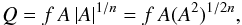$\begin{array}{ccc}\mathit{Q}\mathrm{=}\mathit{f}\hspace{0.17em}\mathit{A}{\left|\mathit{A}\right|}^{\mathrm{1}\mathit{/}\mathit{n}}\mathrm{=}\mathit{f}\hspace{0.17em}\mathit{A}\mathrm{(}{\mathit{A}}^{\mathrm{2}}{\mathrm{)}}^{\mathrm{1}\mathit{/}\mathrm{2}\mathit{n}}\mathit{,}& & \end{array}$(5)with f and n both positive when the Grad-Shafranov equations can be written $\begin{array}{ccc}\frac{{\mathit{\partial }}^{\mathrm{2}}\mathit{A}}{\mathit{\partial }{\mathit{r}}^{\mathrm{2}}}\mathrm{+}\frac{\mathrm{1}}{{\mathit{r}}^{\mathrm{2}}}\mathrm{(}\mathrm{1}\mathrm{-}{\mathit{\mu }}^{\mathrm{2}}\mathrm{)}\frac{{\mathit{\partial }}^{\mathrm{2}}\mathit{A}}{\mathit{\partial }{\mathit{\mu }}^{\mathrm{2}}}\mathrm{+}\frac{\mathit{n}\mathrm{+}\mathrm{1}}{\mathit{n}}\hspace{0.17em}{\mathit{f}}^{\mathrm{2}}\mathit{A}\mathrm{(}{\mathit{A}}^{\mathrm{2}}{\mathrm{)}}^{\mathrm{1}\mathit{/}\mathit{n}}\mathrm{=}\mathrm{0.}& & \end{array}$(6)Equation (6) admits of separable solutions of the form $\begin{array}{ccc}\mathit{A}\mathrm{=}\frac{{\mathit{A}}_{\mathit{n}}\mathrm{\left(}\mathit{\mu }\mathrm{\right)}}{{\mathit{r}}^{\mathit{n}}}\mathit{,}& & \end{array}$(7)with A_n(μ) satisfying the nonlinear ordinary differential equation (ODE) $\begin{array}{ccc}\mathrm{(}\mathrm{1}\mathrm{-}{\mathit{\mu }}^{\mathrm{2}}\mathrm{)}\frac{{\mathrm{d}}^{\mathrm{2}}{\mathit{A}}_{\mathit{n}}}{\mathrm{d}{\mathit{\mu }}^{\mathrm{2}}}\mathrm{+}\mathit{n}\mathrm{(}\mathit{n}\mathrm{+}{\mathrm{1}}^{\mathrm{)}}{\mathit{A}}_{\mathit{n}}\mathrm{+}\frac{\mathit{n}\mathrm{+}\mathrm{1}}{\mathit{n}}\hspace{0.17em}{\mathit{f}}^{\mathrm{2}}{\mathit{A}}_{\mathit{n}}\mathrm{(}{\mathit{A}}_{\mathit{n}}^{\mathrm{2}}{\mathrm{)}}^{\mathrm{1}\mathit{/}\mathit{n}}\mathrm{=}\mathrm{0.}& & \end{array}$(8)Here and in Eq. (7), n can be identified with the decay index discussed in the Introduction.

The geometric condition B_θ = 0 on μ = ± 1 implies that one can set A = 0 along the polar axis, so that one has the homogeneous boundary conditions 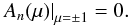$\begin{array}{ccc}{{\mathit{A}}_{\mathit{n}}\mathrm{\left(}\mathit{\mu }\mathrm{\right)}|}_{\mathit{\mu }\mathrm{=}\mathrm{\pm }\mathrm{1}}\mathrm{=}\mathrm{0.}& & \end{array}$(9)Thus Eq. (8)with the boundary conditions (9)forms a nonlinear eigenvalue problem to determine the parameter n. The scale value f can be removed by a simple proportionality factor and therefore plays no role in the eigenvalue problem; one can set f = 1 (or any other convenient value) without loss of generality. However, to track the behavior of various terms through complicated transformations, it is useful to leave f in the eigenvalue equation.

Each solution of the eigenvalue problem provides a magnetic field of the form $\begin{array}{ccc}{B}\mathrm{=}\mathrm{-}\frac{\mathrm{1}}{{\mathit{r}}^{\mathit{n}\mathrm{+}\mathrm{2}}}\left(\frac{\mathrm{d}{\mathit{A}}_{\mathit{n}}}{\mathrm{d}\mathit{\mu }}\mathit{,}\frac{\mathit{n}{\mathit{A}}_{\mathit{n}}}{\sqrt{\mathrm{1}\mathrm{-}{\mathit{\mu }}^{\mathrm{2}}}}\mathit{,}\mathrm{-}\mathit{f}\hspace{0.17em}{\mathit{A}}_{\mathit{n}}\mathrm{(}{\mathit{A}}_{\mathit{n}}^{\mathrm{2}}{\mathrm{)}}^{\mathrm{1}\mathit{/}\mathrm{2}\mathit{n}}\right)\mathit{.}& & \end{array}$(10)Such fields are known as self-similar fields because on any sphere of radius r₀ the flux-profile B_r(r₀,μ) is the same except for a normalization constant. The nonlinear ODE determines such a self-similar flux profile with index n for the radial decay of the global field.

If f = 0, the ODE becomes a linear equation $\begin{array}{ccc}\mathrm{(}\mathrm{1}\mathrm{-}{\mathit{\mu }}^{\mathrm{2}}\mathrm{)}\frac{{\mathrm{d}}^{\mathrm{2}}{\mathit{A}}_{\mathit{n}}}{\mathrm{d}{\mathit{\mu }}^{\mathrm{2}}}\mathrm{+}\mathit{n}\mathrm{(}\mathit{n}\mathrm{+}{\mathrm{1}}^{\mathrm{)}}{\mathit{A}}_{\mathit{n}}\mathrm{=}\mathrm{0}\mathit{,}& & \end{array}$(11)with the familiar Legendre polynomial solutions $\begin{array}{ccc}{\mathit{A}}_{\mathit{n}}\mathrm{\left(}\mathit{\mu }\mathrm{\right)}\mathrm{=}{\mathit{Q}}_{\mathit{n}}\mathrm{\left(}\mathit{\mu }\mathrm{\right)}\mathrm{=}\sqrt{\mathrm{1}\mathrm{-}{\mathit{\mu }}^{\mathrm{2}}}\hspace{0.17em}{\mathit{P}}_{\mathit{n}}^{\mathrm{1}}\mathrm{\left(}\mathit{\mu }\mathrm{\right)}\mathit{,}& & \end{array}$(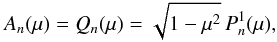12)with n = 1,2,3,..., where ${\mathit{P}}_{\mathit{\ell }}^{\mathit{m}}$ is the associated Legendre polynomial of order ℓ,m. There are no solutions satisfying the boundary conditions when n is not a positive integer. If f ≠ 0, there are, as yet, no known closed-form solutions to the nonlinear eigenvalue problem, so that numerical methods have so far been used as given in LL.

However, there is a mathematical theorem for the nonlinear eigenvalue equation with its associated boundary conditions that helps shed light on the structures allowed for solutions, and this is considered next.

3. Conditions for bipolar field structures

In this section, solutions to the nonlinear equation are investigated that permit dipolar fields. In particular, one requires that the solution be positive (or negative) everywhere, which, as discussed in the following subsection, requires at least 0 <n< 1.

3.1. Integral theorem

Write Eq. (8)in the form $\begin{array}{ccc}& & \frac{\mathrm{d}}{\mathrm{d}\mathit{\mu }}\left[\mathrm{(}\mathrm{1}\mathrm{-}{\mathit{\mu }}^{\mathrm{2}}\mathrm{)}\frac{\mathrm{d}{\mathit{A}}_{\mathit{n}}}{\mathrm{d}\mathit{\mu }}\mathrm{+}\mathrm{2}\mathit{\mu }{\mathit{A}}_{\mathit{n}}\right]\mathrm{+}\left[\mathit{n}\mathrm{(}\mathit{n}\mathrm{+}{\mathrm{1}}^{\mathrm{)}}\mathrm{-}\mathrm{2}\right]{\mathit{A}}_{\mathit{n}}\\ & & \end{array}$(13)Integrate Eq. (13)across −1 <μ< 1 subject to the boundary conditions (9)to obtain $\begin{array}{ccc}\mathrm{(}\mathit{n}\mathrm{+}{\mathrm{2}}^{\mathrm{)}}\mathrm{(}\mathit{n}\mathrm{-}{\mathrm{1}}^{\mathrm{)}}{\mathrm{\int }}_{-1}^{\mathrm{1}}\mathrm{d}\mathit{\mu }\hspace{0.17em}{\mathit{A}}_{\mathit{n}}\mathrm{\left(}\mathit{\mu }\mathrm{\right)}\mathrm{+}\frac{\mathit{n}\mathrm{+}\mathrm{1}}{\mathit{n}}\hspace{0.17em}{\mathit{f}}^{\mathrm{2}}{\mathrm{\int }}_{-1}^{\mathrm{1}}\mathrm{d}\mathit{\mu }{\mathit{A}}_{\mathit{n}}\mathrm{(}{\mathit{A}}_{\mathit{n}}^{\mathrm{2}}{\mathrm{)}}^{\mathrm{1}\mathit{/}\mathit{n}}\mathrm{=}\mathrm{0.}& & \\ & & \end{array}$(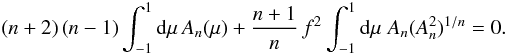14)Now condition (14)rules out the possibility of a bipolar field (i.e., A_n positive or negative everywhere) for n> 1 since both terms are then positive definite or negative definite together. For the case n = 1, treated extensively in LL, one has $\begin{array}{ccc}{\mathrm{\int }}_{-1}^{\mathrm{1}}\mathrm{d}\mathit{\mu }{\mathit{A}}_{\mathit{n}}\mathrm{(}{\mathit{A}}_{\mathit{n}}^{\mathrm{2}}{\mathrm{)}}^{\mathrm{1}\mathit{/}\mathit{n}}\mathrm{=}\mathrm{0}\mathit{,}& & \end{array}$(15)showing that any such eigenfunction (for f ≠ 0) must have at least one zero in −1 <μ< 1.

In the region n< 1 the two terms in Eq. (14)are of opposite sign, so there is no constraint. In particular, one knows from the detailed work reported in LL that dipolar self-similar fields do exist for n< 1. On the other hand, condition (14)is always satisfied for all n> 0 if A_n is an odd function of μ. Note that a zero of A_n corresponds to a purely radial field line separating two bipolar poloidal fields so that any such self-similar solution cannot be dipolar everywhere in −1 <μ< 1.

3.2. Behavior as n → 0

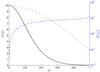Fig. 1 Solutions to the differential Eq. (23). The left vertical axis (black) shows the solution function w(μ) obtained numerically (solid line), the approximation from Eq. (25)neglecting w in Eq. (23)(dot-dashed line), and the approximation for small μ from Eq. (32)(dotted line). The right vertical axis (blue) shows the associated function T(μ).

Fig. 2 Numerical evaluation of the differential Eqs. (26)and (21)for n = 0.4. The left vertical axis (black) shows the result for the function w(μ), while the right vertical axis (blue) shows the absolute values of the function T(μ), with T itself being negative. The solid lines show the result for the initial value, w0, when w0 is less than (upper panel), equal to (middle panel), and greater than (lower panel) the critical value, w0,crit ≈ 5.742. The vertical dotted line in the lower panel marks the critical value μcrit at which T diverges, i.e., |T| → ∞ for μ → μcrit.

One of the more interesting aspects is to provide the behavior of A_n as n → 0. In Eq. (8)write $\begin{array}{ccc}{\mathit{A}}_{\mathit{n}}\mathrm{\left(}\mathit{\mu }\mathrm{\right)}\mathrm{=}\{\begin{array}{c}\\ & \\ & \end{array}& & \end{array}$(16)It is, therefore, sufficient to consider the situation where u is positive. Inserting Eq. (16)into Eq. (8)leads to $\begin{array}{ccc}& & \mathrm{(}\mathrm{1}\mathrm{-}{\mathit{\mu }}^{\mathrm{2}}\mathrm{)}\frac{\mathrm{d}\mathit{u}}{\mathrm{d}{\mathit{\mu }}^{\mathrm{2}}}\mathrm{-}\mathrm{(}\mathrm{1}\mathrm{-}{\mathit{\mu }}^{\mathrm{2}}\mathrm{)}\left(\mathrm{1}\mathrm{-}\frac{\mathit{n}}{\mathrm{2}}\right)\frac{\mathrm{1}}{\mathit{u}}{\left(\frac{\mathrm{d}\mathit{u}}{\mathrm{d}\mathit{\mu }}\right)}^{\mathrm{2}}\\ & & \end{array}$(17)As n → 0, Eq. (17)smoothly reduces to $\begin{array}{ccc}\mathrm{(}\mathrm{1}\mathrm{-}{\mathit{\mu }}^{\mathrm{2}}\mathrm{)}\frac{{\mathrm{d}}^{\mathrm{2}}\mathit{u}}{\mathrm{d}{\mathit{\mu }}^{\mathrm{2}}}\mathrm{-}\mathrm{(}\mathrm{1}\mathrm{-}{\mathit{\mu }}^{\mathrm{2}}\mathrm{)}\frac{\mathrm{1}}{\mathit{u}}{\left(\frac{\mathrm{d}\mathit{u}}{\mathrm{d}\mathit{\mu }}\right)}^{\mathrm{2}}\mathrm{+}\mathrm{2}\mathit{u}\mathrm{+}\mathrm{2}{\mathit{f}}^{\mathrm{2}}{\mathit{u}}^{\mathrm{2}}\mathrm{=}\mathrm{0.}& & \end{array}$(18)To remove the constant f, it is sufficient to introduce $\begin{array}{ccc}\mathit{w}\mathrm{=}{\mathit{f}}^{\mathrm{2}}\mathit{u,}& & \end{array}$(19)when one has $\begin{array}{ccc}\mathrm{(}\mathrm{1}\mathrm{-}{\mathit{\mu }}^{\mathrm{2}}\mathrm{)}\left[\mathit{w}\hspace{0.17em}\frac{{\mathrm{d}}^{\mathrm{2}}\mathit{w}}{\mathrm{d}{\mathit{\mu }}^{\mathrm{2}}}\mathrm{-}{\left(\frac{\mathrm{d}\mathit{w}}{\mathrm{d}\mathit{\mu }}\right)}^{\mathrm{2}}\right]\mathrm{+}\mathrm{2}{\mathit{w}}^{\mathrm{2}}\mathrm{+}\mathrm{2}{\mathit{w}}^{\mathrm{3}}\mathrm{=}\mathrm{0.}& & \end{array}$(20)Make the substitution $\begin{array}{ccc}\frac{\mathrm{d}\mathit{w}}{\mathrm{d}\mathit{\mu }}\mathrm{=}\mathit{w}\mathrm{\left(}\mathit{\mu }\mathrm{\right)}\mathit{T}\mathrm{\left(}\mathit{\mu }\mathrm{\right)}& & \end{array}$(21)so that Eq. (20)yields $\begin{array}{ccc}{\mathit{w}}^{\mathrm{2}}\left[\mathrm{(}\mathrm{1}\mathrm{-}{\mathit{\mu }}^{\mathrm{2}}\mathrm{)}\frac{\mathrm{d}\mathit{T}}{\mathrm{d}\mathit{\mu }}\mathrm{+}\mathrm{2}\mathrm{+}\mathrm{2}\mathit{w}\right]\mathrm{=}\mathrm{0.}& & \end{array}$(22)Equation (22)has two solutions: either w ≡ 0 or $\begin{array}{ccc}\mathrm{(}\mathrm{1}\mathrm{-}{\mathit{\mu }}^{\mathrm{2}}\mathrm{)}\frac{\mathrm{d}\mathit{T}}{\mathrm{d}\mathit{\mu }}\mathrm{+}\mathrm{2}\mathrm{+}\mathrm{2}\mathit{w}\mathrm{=}\mathrm{0.}& & \end{array}$(23)Consider Eq. (23)in the domains where |w| ≪ 1 (such as μ² → 1 when one requires w → 0). Then one has $\begin{array}{ccc}\mathit{T}\mathrm{\left(}\mathit{\mu }\mathrm{\right)}\mathrm{=}{\mathit{T}}_{\mathrm{0}}\mathrm{-}\ln \left(\frac{\mathrm{1}\mathrm{+}\mathit{\mu }}{\mathrm{1}\mathrm{-}\mathit{\mu }}\right)\mathit{,}& & \end{array}$(24)where T₀ is an arbitrary constant. It follows from Eq. (21)that, if |w| ≪ 1, one has $\begin{array}{ccc}\mathit{w}\mathrm{=}\frac{{\mathit{w}}_{\mathrm{0}}}{\mathrm{1}\mathrm{-}{\mathit{\mu }}^{\mathrm{2}}}{\left(\frac{\mathrm{1}\mathrm{-}\mathit{\mu }}{\mathrm{1}\mathrm{+}\mathit{\mu }}\right)}^{\mathit{\mu }}\hspace{0.17em}\exp \left({\mathit{T}}_{\mathrm{0}}\mathit{\mu }\right)\mathit{,}& & \end{array}$(25)where w₀ is a constant. However, Eq. (25)does not admit of w → 0 as μ² → 1 unless w₀ is itself zero. Thus the only remaining solution that is smoothly continuous as n → 0 is w ≡ 0.

Fig. 3 Critical initial value w0,crit as n is varied. The shaded area above the curve marks the region where no solution can be obtained that reaches to μ = 1.

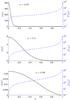Fig. 4 Numerical evaluation of the differential Eqs. (26)and (21)for n = 0.05 (upper panel), n = 0.4 (middle panel), and n = 0.99 (lower panel). For each sub-figure, the left vertical axes (black) show the result for the function w(μ), while the right vertical axes (blue) show the absolute values of the function T(μ). The black solid and blue dashed lines show the numerically evaluated functions w(μ) and |T(μ)|, respectively, while the black dotted line shows the approximate result from Eq. (32). In each case, the critical value w0,crit has been used for the parameter w0 (see Fig. 3).

Fig. 5 Critical value μcrit for the domain permitting a solution to the differential Eqs. (26)and (21)as n and w0 are varied.

Numerically, it can be shown that the contribution of the so far neglected contribution by the function w in Eq. (22)indeed changes the picture. However, the initial value, w₀, has to be large compared to unity to allow for a solution that asymptotically vanishes as μ² → 1, thereby contradicting the assumption that led to the approximate solution in Eq. (25). This result is illustrated in Fig. 1.

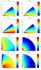Fig. 6 Magnetic field components based on Eq. (3)for a cut through the x–z plane. Shown are the cases of n = 0.05 (upper four panels) and of n = 0.99 (lower four panels), both for w0 = w0,crit. For each case, the panels represent the magnetic field components and the total field strength, all scaled logarithmically. For n = 0.05, the solution falls toward zero rapidly so that the corresponding parts are left blank in the logarithmic plot.

3.3. Approximate analytical evaluation

Based on Eq. (17), one can quite generally write $\begin{array}{ccc}\mathrm{(}\mathrm{1}\mathrm{-}{\mathit{\mu }}^{\mathrm{2}}\mathrm{)}\frac{\mathrm{d}\mathit{T}}{\mathrm{d}\mathit{\mu }}\mathrm{+}\mathrm{2}\mathrm{(}\mathrm{1}\mathrm{+}{\mathit{n}}^{\mathrm{)}}\mathrm{(}\mathrm{1}\mathrm{+}{\mathit{w}}^{\mathrm{)}}\mathrm{+}\frac{\mathit{n}}{\mathrm{2}}\mathrm{(}\mathrm{1}\mathrm{-}{\mathit{\mu }}^{\mathrm{2}}\mathrm{)}{\mathit{T}}^{\mathrm{2}}\mathrm{=}\mathrm{0}\mathit{,}& & \end{array}$(26)which is valid for arbitrary n.

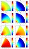Fig. 7 Magnetic field components based on Eq. (3)for a cut through the x–z plane. Shown are the cases of n = 0.4 with w0 = 3 <w0,crit (upper four panels) and w0 = 8 >w0,crit (lower four panels). For each case, the panels represent the magnetic field components and the total field strength, all scaled logarithmically. For w0>w0,crit, the solution does not reach to μ = 1 so that for high latitudes no magnetic field is available.

Note that in any domain where |w| ≪ 1 Eq. (26)reduces to $\begin{array}{ccc}\mathrm{(}\mathrm{1}\mathrm{-}{\mathit{\mu }}^{\mathrm{2}}\mathrm{)}\left(\frac{\mathrm{d}\mathit{T}}{\mathrm{d}\mathit{\mu }}\mathrm{+}\frac{\mathit{n}}{\mathrm{2}}\hspace{0.17em}{\mathit{T}}^{\mathrm{2}}\right)\mathrm{+}\mathrm{2}\mathrm{(}\mathrm{1}\mathrm{+}{\mathit{n}}^{\mathrm{)}}\mathrm{=}\mathrm{0.}& & \end{array}$(27)With the substitution $\begin{array}{ccc}\mathit{T}\mathrm{=}\frac{\mathrm{2}}{\mathit{n}}\hspace{0.17em}\frac{\mathrm{d}\mathit{y}}{\mathrm{d}\mathit{\mu }}\hspace{0.17em}\frac{\mathrm{1}}{\mathit{y}}& & \end{array}$(28)one then has $\begin{array}{ccc}\mathrm{(}\mathrm{1}\mathrm{-}{\mathit{\mu }}^{\mathrm{2}}\mathrm{)}\frac{{\mathrm{d}}^{\mathrm{2}}\mathit{y}}{\mathrm{d}{\mathit{\mu }}^{\mathrm{2}}}\mathrm{+}\mathit{n}\mathrm{(}\mathit{n}\mathrm{+}{\mathrm{1}}^{\mathrm{)}}\mathit{y}\mathrm{=}\mathrm{0.}& & \end{array}$(29)One is interested in the even solutions to Eq. (29)only because odd solutions would automatically have a location (i.e., μ = 0) where the solution would be zero and so no dipolar field is possible. For even solutions one has dy/ dμ = 0 on μ = 0. Furthermore, it is sufficient to consider solutions in μ> 0 only from symmetry considerations and also sufficient to consider those solutions with y> 0 on μ = 0. Under these conditions, the solution to Eq. (29)can be written in closed analytical form as $\begin{array}{ccc}\mathit{y}\mathrm{\left(}\mathit{\mu }\mathrm{\right)}\mathrm{=}{\mathit{y}}_{\mathrm{0}}2\mathit{F}1\left(\mathrm{-}\frac{\mathrm{1}\mathrm{+}\mathit{n}}{\mathrm{2}}\mathit{,}\frac{\mathit{n}}{\mathrm{2}}\mathit{,}\frac{\mathrm{1}}{\mathrm{2}}\mathit{,}{\mathit{\mu }}^{\mathrm{2}}\right)\mathit{,}& & \end{array}$(30)where 2F1 is the hypergeometric function (e.g., Gradshteyn & Ryzhik 2000). However, y(μ) from Eq. (30)allows for y( ± 1) = 0 if, and only if, n = 1.

There remain then two options: (i) either |w| is not much smaller than unity everywhere as postulated; or (ii) the solutions are bounded to domains of μ (for instance, −μ_⋆<μ<μ_⋆) that are smaller than −1 <μ< 1 and solutions are discontinuously joined outside of such domains. Under such conditions one can have a discontinuous matching of solutions so that dy/ dμ is negative on μ = μ_⋆ when approached from μ<μ_⋆ with y starting again from zero for μ>μ_⋆. It will now be shown that both the first option is true, meaning that |w| ≪ 1 cannot be justified, and the second option is also true, that is, limited spatial domain solutions.

3.4. Numerical evaluation

To study the global behavior of the solution over the entire domain −1 <μ< 1, it is shown here that it is imperative not to neglect the term w that led to the approximation (27). Instead, consider first the domain near μ = 0.

Expand T ≈ T₁μ and w ≈ w₀ with T₁ and w₀ constant. Then, to first order in μ, one has from Eq. (26)$\begin{array}{ccc}{\mathit{T}}_{\mathrm{1}}\mathrm{=}\mathrm{-}\mathrm{2}\mathrm{(}\mathrm{1}\mathrm{+}{\mathit{n}}^{\mathrm{)}}\mathrm{(}\mathrm{1}\mathrm{+}{\mathit{w}}_{\mathrm{0}}\mathrm{)}\mathit{.}& & \end{array}$(31)When inserted into the definition of T, that is, Eq. (21), one finds $\begin{array}{ccc}\mathit{w}\mathrm{=}{\mathit{w}}_{\mathrm{0}}\exp \mathrm{[}\mathrm{-}{\mathit{\mu }}^{\mathrm{2}}\mathrm{(}\mathrm{1}\mathrm{+}{\mathit{n}}^{\mathrm{)}}{\mathrm{(}\mathrm{1}\mathrm{+}{\mathit{w}}_{\mathrm{0}}\mathrm{)}}^{\mathrm{]}}\mathit{,}& & \end{array}$(32)again valid for μ ≪ 1. Accordingly, the solution w(μ) depends nonlinearly on both n and on the initial value w₀, which is confirmed by the numerical solution shown below.

The coupled system of differential equations, Eqs. (26)and (21), is solved using the Bulirsch-Stoer method (Stoer & Bulirsch 2002), which is a modified mid-point method combining the ideas of Richardson extrapolation and rational function extrapolation. This method has its strengths particularly if high accuracies are required (cf. Press et al. 2007). In addition, the method allows one to control the local truncation error by adapting the step size. Here the maximum tolerance per step size is taken to be one part in 10¹⁵.

For the example of n = 0.4, the resulting solutions w(μ) and T(μ) are shown in Fig. 2 using three different initial values w₀. As shown, there exists a critical initial value, w_0,crit, above which the function T goes to minus infinity, T(μ) → −∞ for μ → μ_crit with μ_crit< 1. The dependence of μ_crit on n and w₀ is illustrated in Fig. 5, showing that, to obtain a solution that reaches to μ = 1, either n or w₀ (or both) have to be small.

By repeating the same evaluations for varying n ∈ [ 0,1 ], Fig. 3 shows that the critical initial value, w_0,crit, depends sensitively on the parameter n with w_0,crit → 0 for n → 1. This result agrees with the argument in Sect. 3.1 that for , no bipolar solution is possible.

Additional examples are shown in Fig. 4, each for the critical initial value w_0,crit. In addition, Fig. 4 illustrates that for intermediate values of n (for example, n = 0.4), the approximate solution from Eq. (32)agrees surprisingly well with the numerical solution.

3.5. Alternative analytical approach

As shown in the previous subsections, while there are allowed bipolar solutions in n< 1, such solutions have a limited range for μ above a critical value for w(μ = 0).

An alternative is to set up a variational principle. One can carry through this variational principle calculation following standard methods, therefore we do not need to repeat them here.

4. Discussion and conclusion

A major challenge to increase the understanding of long-lived magnetic fields in the solar corona (that have often been described through force-free fields that are everywhere aligned with their current densities) is related to the complex nature of the nonlinear equations describing such behaviors. When the equations are separable, there results a highly nonlinear eigenvalue problem that is somewhat intractable analytically and that depends sensitively on the rate of radial decrease of the poloidal component of the magnetic field, given by r^{− n}. The parameter n can be identified with the decay index and is greater than or equal to zero.

The resulting magnetic field components are illustrated in Figs. 6 and 7 for several values of the index n and the initial value w₀. Likewise, Fig. 8 illustrates the pattern resulting from the direction of the axisymmetric magnetic field.

If attention is focused on purely dipolar fields, then any such dipolar behaviors are shown to be limited to n< 1, else one must have multipole behaviors. Even in the domain where n< 1, there is not complete freedom in obtaining a dipolar field when w exceeds a critical value as a function of n, as shown in Fig. 2.

Dipolar solutions only exist within restricted ranges of the angular coordinate θ. This pattern of behavior is firmly tied to the nonlinearity of the basic equations, because if the nonlinear terms are set exactly to zero, then there are indeed dipolar solutions stretching across the total range −1 < cosθ< 1.

The results obtained here should be of use in attempts to consider the problem in more depth and also may provide guidance when one attempts to address the considerably more complex problem of 3D non-axisymmetric force-free fields on a sphere.

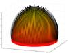Fig. 8 Visualization of the magnetic field pattern (in arbitrary units) for n = 0.4 with w0 = 3 <w0,crit as obtained from Eq. (3). The arrows merely indicate the magnetic field direction and are re-scaled for clarity so that their length does not reflect the magnetic field strength.

Acknowledgments

B.C. Low is thanked profusely for his unending support and help and for suggesting this problem. It would have been most appropriate if he had been able to co-author this paper, but his massive commitments to other works just prior to his retirement took their toll on his ability to participate.

References

All Figures

	Fig. 1 Solutions to the differential Eq. (23). The left vertical axis (black) shows the solution function w(μ) obtained numerically (solid line), the approximation from Eq. (25)neglecting w in Eq. (23)(dot-dashed line), and the approximation for small μ from Eq. (32)(dotted line). The right vertical axis (blue) shows the associated function T(μ).
In the text

Fig. 2 Numerical evaluation of the differential Eqs. (26)and (21)for n = 0.4. The left vertical axis (black) shows the result for the function w(μ), while the right vertical axis (blue) shows the absolute values of the function T(μ), with T itself being negative. The solid lines show the result for the initial value, w0, when w0 is less than (upper panel), equal to (middle panel), and greater than (lower panel) the critical value, w0,crit ≈ 5.742. The vertical dotted line in the lower panel marks the critical value μcrit at which T diverges, i.e., |T| → ∞ for μ → μcrit.

In the text

	Fig. 3 Critical initial value w0,crit as n is varied. The shaded area above the curve marks the region where no solution can be obtained that reaches to μ = 1.
In the text

Fig. 4 Numerical evaluation of the differential Eqs. (26)and (21)for n = 0.05 (upper panel), n = 0.4 (middle panel), and n = 0.99 (lower panel). For each sub-figure, the left vertical axes (black) show the result for the function w(μ), while the right vertical axes (blue) show the absolute values of the function T(μ). The black solid and blue dashed lines show the numerically evaluated functions w(μ) and |T(μ)|, respectively, while the black dotted line shows the approximate result from Eq. (32). In each case, the critical value w0,crit has been used for the parameter w0 (see Fig. 3).

In the text

	Fig. 5 Critical value μcrit for the domain permitting a solution to the differential Eqs. (26)and (21)as n and w0 are varied.
In the text

Fig. 6 Magnetic field components based on Eq. (3)for a cut through the x–z plane. Shown are the cases of n = 0.05 (upper four panels) and of n = 0.99 (lower four panels), both for w0 = w0,crit. For each case, the panels represent the magnetic field components and the total field strength, all scaled logarithmically. For n = 0.05, the solution falls toward zero rapidly so that the corresponding parts are left blank in the logarithmic plot.

In the text

Fig. 7 Magnetic field components based on Eq. (3)for a cut through the x–z plane. Shown are the cases of n = 0.4 with w0 = 3 <w0,crit (upper four panels) and w0 = 8 >w0,crit (lower four panels). For each case, the panels represent the magnetic field components and the total field strength, all scaled logarithmically. For w0>w0,crit, the solution does not reach to μ = 1 so that for high latitudes no magnetic field is available.

In the text

	Fig. 8 Visualization of the magnetic field pattern (in arbitrary units) for n = 0.4 with w0 = 3 <w0,crit as obtained from Eq. (3). The arrows merely indicate the magnetic field direction and are re-scaled for clarity so that their length does not reflect the magnetic field strength.
In the text

References

- Cheng, X., Zhang, J., Ding, M. D., Guo, Y., & Su, J. T. 2011, ApJ, 732, 87 [NASA ADS] [CrossRef] [Google Scholar]
- Filippov, B., Martsenyuk, O., Srivastava, A. K., & Uddin, W. 2015, JApA, 36, 157 [Google Scholar]
- Gradshteyn, I. S., & Ryzhik, I. N. 2000, Table of Integrals, Series, and Products (London: Academic Press) [Google Scholar]
- Lerche, I., & Low, B. C. 2014, Phys. Plasmas, 21, 102902 [NASA ADS] [CrossRef] [Google Scholar]
- Liu, Y. 2008, ApJ, 679, L151 [NASA ADS] [CrossRef] [Google Scholar]
- Low, B. C., & Lou, Y. O. 1990, ApJ, 352, 343 [NASA ADS] [CrossRef] [Google Scholar]
- Nindos, A., Patsourakos, S., & Wiegelmann, T. 2012, ApJ, 748, L6 [NASA ADS] [CrossRef] [Google Scholar]
- Press, W. H., Teukolsky, S. A., Vetterling, W. T., & Flannery, B. P. 2007, Numerical Recipes (Cambridge University Press) [Google Scholar]
- Stoer, J., & Bulirsch, R. 2002, Introduction to Numerical Analysis, 3rd edn. (New York: Springer) [Google Scholar]
- Wang, H., Cao, W., Liu, C., et al. 2015, Nature Commun., 6, 7008 [Google Scholar]