| Issue |
A&A
Volume 581, September 2015
|
|
|---|---|---|
| Article Number | A123 | |
| Number of page(s) | 9 | |
| Section | Galactic structure, stellar clusters and populations | |
| DOI | https://doi.org/10.1051/0004-6361/201526516 | |
| Published online | 21 September 2015 | |
Quasi integral of motion for axisymmetric potentials
1
Observatoire astronomique de Strasbourg, Université de Strasbourg, CNRS,
UMR 7550, 11 rue de l’Université,
67000
Strasbourg,
France
e-mail:
This email address is being protected from spambots. You need JavaScript enabled to view it.
2
Institut Utinam, CNRS UMR 6213, Université de Franche-Comté, OSU
THETA Franche-Comté-Bourgogne, Observatoire de Besançon, BP 1615, 25010
Besançon Cedex,
France
Received: 12 May 2015
Accepted: 20 July 2015
Abstract
We present an estimate of the third integral of motion for axisymmetric three-dimensional potentials. This estimate is based on a Stäckel approximation and is explicitly written as a function of the potential. We tested this scheme for the Besançon Galactic model and two other disc-halo models and find that orbits of disc stars have an accurately conserved third quasi integral. The accuracy ranges from of 0.1% to 1% for heights varying from z = 0 kpc to z = 6 kpc and Galactocentric radii R from 5 to 15 kpc. We also tested the usefulness of this quasi integral in analytic distribution functions of disc stellar populations: we show that the distribution function remains approximately stationary and that it allows to recover the potential and forces by applying Jeans equations to its moments.
Key words: methods: numerical / Galaxy: kinematics and dynamics
© ESO, 2015
1. Introduction
Many approaches exist for the galactic modelling of stellar dynamics. With the availability of a large amount of new accurate data for the velocity and position of stars in the extended solar neighbourhood, the development of the most precise tools for analysing the kinematics of stars is becoming inescapable.
Numerical modelling techniques are the most direct ones, such as for the Scharwschild method, the made-to-measure method (Syer & Tremaine 1996), or of course ab initio N-body and hydrodynamical simulations (Renaud et al. 2013). Spectral analysis (Papaphilippou & Laskar 1998; Valluri & Merritt 1998) also offers useful numerical tools for recognising and identifying resonances. Numerical resolution of the collisionless Boltzmann equation is another direct way to model, but it is still limited by available numerical resources (Yoshikawa et al. 2013; Colombi et al. 2015).
Analytical techniques are more explicit but imply analytical approximations. In the case of axisymmetric galactic potentials, it is known that orbits are generally constrained by an effective third integral of motion in addition to the energy and angular momentum. From the Jeans theorem, therefore, equilibrium models of axisymmetric galaxies should be represented by distribution functions that only depend on these three integrals. The modelling of stellar distribution functions can thus be achieved if the effective third integral can be approximated analytically or numerically.
A long list of works in this direction already exists, and very useful bibliographies may be found in de Zeeuw (1985), de Zeeuw & Lynden-Bell (1985), De Bruyne et al. (2000), Binney (2012), and Sanders & Binney (2014), among others. We concentrate here on the use of Stäckel potentials that have been shown in many cases to be efficient for modelling different families of orbits. Published works on this subject present a wide variety of approaches, and we can distinguish between the local and global approaches. The local modelling consists in locally fitting the true potential with a Stäckel potential. This allows nearly exact modelling of orbits and integrals of motion to be obtained in the immediate neighbourhood of the position considered.
Global modelling, either of the potential or of the orbits over a predefined phase-space volume, has opened the way to many different technicalities over the past 50 yr. In each case the goal was to use a Stäckel third integral as an approximate of the third quasi integral of the fitted potential, as in Wayman (1959), van de Hulst (1962), Ollongren (1962), Hori (1962), and more recently, Manabe (1979), Batsleer & Dejonghe (1994), or Famaey & Dejonghe (2003).
A recent novel application of the Stäckel potential approximations has been to model the local stellar kinematics and the gravitational potential in the solar neighbourhood at large z distances up to 1−2 kpc from the galactic plane (Bienaymé et al. 2014; Piffl et al. 2014). These recent studies put strict constraints on the vertical variation in the gravitational potential and in the local density of the dark matter halo. Recently, Sanders & Binney (2014) have proposed a global Stäckel fitting of 3D potentials, and they give algebraic expressions that allow recovery of the integrals of motion, expressed as action variables, and they present numerical applications.
In the present paper, we proceed to a Stäckel potential fitting by using a simple expression for the integral of motion that explicitly depends on the potential. Our study has similarities with the works recently published by Binney (2012) or by Sanders & Binney (2014), proposing different formulations of a third integral. Although there are also advantages in working with action integrals, the present approach is, however, much simpler and more straightforward to apply.
The paper proceeds as follows. In Sect. 2, we give a new expression for the third integral, and its derivation is described in the Appendix. In Sect. 3 we examine, for three potentials, the constancy of this third integral along orbits. Section 4 shows, in the case of the Besançon Galactic model, how moments of distribution functions based on this third integral are in accordance with Jeans equations. Section 5 finally considers the application to the collisionless Boltzmann equation.
2. Quasi integral of motion
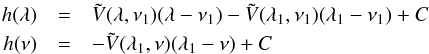
We let V(R,z) be an axisymmetric gravitational potential. Besides the energy E and the vertical component of the angular momentum Lz, which are integrals of motion, we define here, as an approximate third integral of motion,  (1)where L and Lz are the total and vertical angular momenta, z0 a fixed parameter at fixed E and Lz, vz the vertical velocity, and with
 ![Mathematical equation: \begin{equation} \label{eq2} \Psi(R,z)=- \left[ V (R,z) - V(\sqrt{\lambda},0 )\right] \, \frac{(\lambda +z_0^2)} {z_0^2} , \end{equation}](/articles/aa/full_html/2015/09/aa26516-15/aa26516-15-eq14.png) (2)and
(2)and  (3)This approximate integral Is is an exact integral in the case of Stäckel potentials expressed in an ellipsoidal coordinate system of focus z0, which is thus a known quantity. Its derivation is explained in the Appendix.
The only free quantity for determining Is, when V(R,z) is known, is the parameter z0. Here, it will be numerically adjusted by minimizing σIs the dispersion of the quasi integral Is along all the orbits with the same energy and vertical angular momentum. Thus z0 will itself be a function of the two integrals E and Lz.
In a preliminary analysis, which was not developed further, we used the generic differential equation of Stäckel potentials that can be rewritten to determine z0 locally as a function of the second derivatives of the potential at any positions (see Eq. (10) in Bienaymé 2009; de Zeeuw 1985). However, we find out that such a procedure gives us significantly fewer accurate results than fitting a single z0 for a given orbit or family of orbits. Here, we look for the z0 value that minimizes the dispersion of Is along each orbit of a family of orbits with the same E and Lz. We note, however, that for any (E, Lz)-family of orbits and with zshell being the maximum z-extent of the shell orbit, the value of z0 that gives the best fit is close to the value of z0 obtained by applying Eq. (10) of Bienaymé (2009) at position (Rc,zshell/ 2) (with Rc(Lz) the radius of the circular orbit with angular momentum Lz).
The degree of the approximation of the quasi integral Is can be controlled in several ways: (1) inspection of the surfaces of section; (2) conservation of orbital weights and of the spatial density; and (3) conservation of Is along the orbits to validate the labelling of orbits. The conservation of orbital weights and the conservation of Is are the criteria that can be best expressed numerically.
In the following sections, we test the degree of conservation of this quasi integral along orbits in the cases of three non-Stäckel potentials. We also determine its efficiency to build stationary stellar disc distribution functions and to measure the potential from the Jeans equations.
3. Testing the conservation of the integral along orbits
We examined the conservation of the quasi-integral of motion along orbits of stars corresponding to disc stellar populations. For these disc components, stellar motions have restricted oscillations in the radial and vertical directions. For the smallest oscillations, the phase-space domain explored by stars is the closest to a Stäckel potential, and the quasi integral tends to be constant.
We considered stars with identical angular momentum Lz (with Ec the energy of the corresponding circular orbit) and identical energy E (we define ΔE = E − Ec). For each star, we computed the mean value of Is and its dispersion σIs from ~10 000 steps along the orbit, and we determined the value of z0 that minimizes σIs. To ensure that σs is determined sufficiently well, the total time integration for each orbit is about 300 dynamical times (i.e. 300 galactic rotations). The numerical integration is a Runge-Kutta-Fehlberg of order 7(8) (Fehlberg 1968). We find that stellar orbits with the same values of Lz and ΔE all have σIs minimum for similar values of z0. For different energies and angular momenta, the adjusted z0 will be different.
To allow an easier presentation of our results, we normalized Is as  (4)still an integral of motion. I3 = 0 corresponds to orbits confined within the galactic plane, while I3 ~ 1 corresponds to shell orbits with minimum radial variations when they cross the plane z = 0.
In the following sections, we consider three potentials: a logarithmic potential with a disc component, a flattened logarithmic potential, and a potential similar to the Besançon Galactic model potential. In all the three cases, the constancy of the third integral is satisfied at 0.2 to 0.5 per cent for orbits corresponding to thin or thick stars and to a 1 to 2 per cent for orbits with larger vertical oscillations.
3.1. Logarithmic potential of Myamoto-Nagai type
The logarithmic potential of Myamoto-Nagai type  (5)has a positive density (Zotos 2011). It has a spherical halo and a disc component (with a + b the halo core radius and b the disc thickness). This potential presents analogy with the family of density-potential pairs of logarithmic Myamoto-Nagai type given by Bienaymé (2009).
We consider the orbits with the angular momentum Lz = 8.5 (v∞ = 1, a = 0.5, b = 0.2, Rc = 8.5) and with E = Ec + ΔE. The initial conditions of the computed orbits are vR = 0, with Rinitial equally spaced. These initial conditions do not include resonant orbits that do not cross the galactic plane perpendicularly.
Table 1 summarizes the results. For each energy ΔE, the adjusted z0 that minimizes σI3 is given. The maximum vertical extension zmax corresponds to an orbit with I3 close to 1. The dispersions of I3 always remain small, the mean dispersion being smaller than one per cent. However, for some resonant orbits, the dispersion is larger, of the order of 2 per cent. We also note that at large energies corresponding to halo stars the variation of I3 still remains small. This must be linked to the spherical shape of the potential at large z, easily modelled by a Stäckel potential.
Disc-halo logarithmic potential.
In the next section we consider a different requirement using a flattened potential.
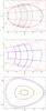 |
Fig. 1 Top panel: meridional projection for three orbits within the logarithmic potential (Sect. 3.2) with Lz = 8.5 and ΔE = 0.2. Zero velocity curve and some coordinate curves of the elliptic coordinates (with z0 = 5.9) are drawn. Middle panel: analytical determination of the envelopes of the orbits. Bottom panel: surfaces of section for the same three orbits. Black crosses: numerically computed orbits. Red lines: the corresponding sections obtained from Eqs. (1)−(3). Blue line: surface of section of the orbit confined in the mid-plane (i.e. vz = 0). |
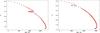 |
Fig. 2 Left: quasi integral I3 versus zmax for stars with ΔE = 6400 and Rc(Lz) = 8500 pc for the BGM potential. Errors bars are σI3. Right: idem with ΔE = 12 800. |
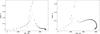 |
Fig. 3 Left: dispersion σI3 of the integral I3 along orbits versus zmax for stars with ΔE = 6400 and Rc(Lz) = 8500 for the BGM potential. Right: idem with ΔE = 12 800. |
3.2. Logarithmic potential
To examine the impact of the flattening of the dark halo on the dispersions σI3, we consider the traditional logarithmic potential Richstone (1980):  (6)We set vc = 1 and q = 0.8 to correspond to a flattening of the isodensity qρ = 0.65.
We computed orbits with Lz = 8.5 (Rc = 8.5, Ec = 1). Table 2 summarizes the results. Surfaces of section for Lz = 1, ΔE = 0.05, and 0.5 are shown in Fig. 9 of Bienaymé & Traven (2013), and we note the lack of resonant orbits. This may explain the excellent conservation of I3 at a level of 0.2 per cent for stellar disc orbits. Orbits with larger extension up to zmax = 9 (E = 0.4) have I3 conserved at 2 per cent.
The inspection (see Fig. 1) of the surface of section and of the meridional projection of three orbits (ΔE = 0.2 and Lz = 8.5) allows visualization of the relative agreement between the nearly exact numerical orbits and the contours obtained from the approximated third integral. For the meridional projection, the red dashed lines are ellipsoids and hyperboloids from the ellipsoidal coordinates with z0 = 5.9 (lines are drawn from the corner of the orbit envelopes). The blue continuous lines in Fig. 1 (middle panel) are the envelopes that are determined semi-analytically from E, Lz and the quasi integral I3 that are explicitly known: we determine surfaces of section at various fixed R (resp. fixed z) and find the z (resp. R) extension limits of the orbit from the condition ∂I3/∂vr = 0 (resp. ∂I3/∂vz = 0). We note small differences between the envelopes of numerical orbits (top panel) and semi-analytical envelopes (middle panel). We also note that the analytical hypersurfaces defined from E, I3 do not have the topology of a torus everywhere. The bottom panel of Fig. 1 shows a section of the phase space (z = 0) for the same three orbits from the numerically computed orbits and from the analytical section given by Eq. (1). If vc = 200 km s-1, the maximum vR of these three orbits is ~120, 50, and 20 km s-1.
3.3. The Besançon Galactic mass model
We apply our test to the gravitational potential of the Besançon Galactic model (BGM; Bienaymé et al. 1987; Robin et al. 2003; Czekaj et al. 2014), which is a more realistic one than the two previous ones, although we limited our analysis to its axisymmetric version. This model has a dynamical consistency at the solar Galactic radius position in the sense that the thickness of the stellar components are constrained by the potential and by the vertical velocity dispersions. However, outside of the solar neighbourhood, the vertical kinematics and the thickness of stellar components are constrained by observations and not by a dynamical consistency of the model. The motivation of this work is to improve the BGM dynamical consistency by using stationary distribution functions to model the stellar kinematics. Besides the integrals E and Lz, we therefore require an approximate third integral to describe the stellar kinematics.
We determined the gravitational potential of the Besançon Galactic model according to the characteristics of its components described in Robin et al. (2003) and Czekaj et al. (2014). The dark matter component is represented by a spherical component. The orbits with large vertical extensions have shapes that are mainly determined by the spherical halo. Since the exact shape of the dark halo remains uncertain in practice and is a controversial question, we consider a less favourable situation using a flattened dark matter component.
The dark matter halo density used in the BGM is  (7)We flatten the halo, replacing the quantity R with
  in the expression of the potential. With Rcore = 2700 pc and q = 0.8, the flattening of the density is qρ = 0.62. (For this value of q, negative densities only occur in a region far from our domain of interest.)
We also modify the point-mass bulge (Bienaymé et al. 1987) using the potential law  with Rbulbe = 2000 pc.
Logarithmic potential (see legend of Table 1).
We summarize the results for orbits with Lz corresponding to Rc = 8500 pc in Table 3. Results are listed by families of different energies ΔE. Figure 2 shows I3 versus zmax, the maximum vertical extension of orbits in cases ΔE = 6400 or 12 800 and Rc = 8500 pc. Error bars are the dispersion of I3 along each orbit. The dispersion of I3 is zero for orbits confined in the mid-plane. Shell orbits have I3 maximum and σI3 close to a few 10-4 (Fig. 3). This is unexpected since there is no reason that the potential along the “thin” orbits should have exactly the Stäckel form. On the other hand, when zmax ~ 2000 pc, the dispersion of I3 is maximum and increases sharply for all energies (see Fig. 3), also corresponding in Fig. 2 to a change of shape of the distribution of points. This is related to the presence of (1, 1) resonant orbits at this vertical height that are poorly modelled by our Stäckel adjustment. For these orbits the dispersion of the quasi integral is less than 5 per cent. The median dispersion of I3 for orbits with zmax smaller than 2 kpc remains very small ~0.002.
We performed the Stäckel adjustment for other galactic radii Rc from 1.5 to 15 kpc. For each pair of values (E = Ec + ΔE, Lz), we determine the z0 value that minimizes σI3. Figure 4 plots the fitted z0 (crosses) for ΔE = 100, 200, 400...12 800. Lines of constant ΔE are plotted. We obtain a tabulation of z0 that gives us a function of two integrals of motion z0(E,Lz) that can be used to build a distribution function for stellar populations.
The median dispersions of I3 remain low except at galactic radii smaller than 3 kc where many resonant orbits dominate the phase space. Figure 5 plots the histograms of σI3 for Rc from 3.5 to 15.5 kpc.
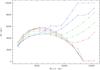 |
Fig. 4 BGM potential: z0 best fit versus Rc(Lz) and ΔE. Black lines ΔE = 100 and 200; red lines: 400 and 800; green lines: 1600 and 3200; blue lines: 64 000 and 128 000. |
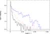 |
Fig. 5 Histograms of I3 dispersion along orbits for zmax intervals delimited by 0, 1000 pc, 2000 pc, and beyond (respectively black, dotted red, dashed blue lines). For each of the three zmax intervals, the medians of σI3 are respectively 5 × 10⁻⁴, 1.5 × 10⁻³, and 5 × 10⁻³. |
4. Distribution function and Jeans equations
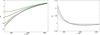 |
Fig. 6 Left: dark lines: radial forces KR of the BGM at several z above the galactic plane (0.5, 1, 2, and 3 kpc, bottom to top). Thin green lines: KR recovered from a Jeans equation in the case of a thick disc. Thin red lines: the case of a thin disc. Right: relative errors on the recovered radial force KR versus R at various z (0.5, 1, 2, and 3 kpc; resp. green, black, red, and blue lines) for thin disc DF (dotted lines) and thick disc DF (continuous lines). |
We tested the efficiency of using the quasi integral I3 to model the distribution function of disc stars using a Shu distribution function (DF) generalized to 3D axisymmetric potentials. It writes as (here, we correct a typographic error in Bienaymé 1999): ![Mathematical equation: \begin{eqnarray} \label{eq8} f(E,L_z, I_3) = &&\frac{2\Omega(R_{\rm c})}{ 2\pi\kappa(R_{\rm c})} \frac{\Sigma(L_z)}{ \sigma_R^2 } \exp \left[ -\frac{ \left(E-E_{\rm circ}\right)}{\sigma_R^2} \right] \nonumber\\ && \times \frac{ 1}{ \sqrt{2\pi} } \frac{1}{\sigma_z } \exp \left[ -\left( E-E_{\rm circ} \right) \left( \frac{1}{\sigma_z^2}-\frac{1}{\sigma_R^2} \right) I_3 \right] . \end{eqnarray}](/articles/aa/full_html/2015/09/aa26516-15/aa26516-15-eq93.png) (8)with Rc(Lz) the radius of the circular orbit with the angular momentum Lz, Ω the angular velocity, κ the epicyclic frequency, and Ecirc the energy of a circular orbiting star at radius Rc. For sufficiently small velocity dispersions, the number density distribution, Σ(Lz) = Σ0exp(−Rc/Rν), is close to Σ(R) = Σ0exp(−R/Rν). We set constant the parameters σR,z(Lz) and Rν = 2.5 kpc, which is close to the scale length of the number density distribution. The DF allows us to reproduce the triaxiality and tilt of the velocity ellipsoid and to model nearly exponential density disc distribution. It could be easily modified to reproduce any reasonable radial density law. We set a constant velocity dispersion (RσR,z = ∞) for a thin disc (σR,σz) = (40 km s-1, 20 km s-1) and for a thick disc (σR,σz) = (60 km s-1, 40 km s-1).
(8)with Rc(Lz) the radius of the circular orbit with the angular momentum Lz, Ω the angular velocity, κ the epicyclic frequency, and Ecirc the energy of a circular orbiting star at radius Rc. For sufficiently small velocity dispersions, the number density distribution, Σ(Lz) = Σ0exp(−Rc/Rν), is close to Σ(R) = Σ0exp(−R/Rν). We set constant the parameters σR,z(Lz) and Rν = 2.5 kpc, which is close to the scale length of the number density distribution. The DF allows us to reproduce the triaxiality and tilt of the velocity ellipsoid and to model nearly exponential density disc distribution. It could be easily modified to reproduce any reasonable radial density law. We set a constant velocity dispersion (RσR,z = ∞) for a thin disc (σR,σz) = (40 km s-1, 20 km s-1) and for a thick disc (σR,σz) = (60 km s-1, 40 km s-1).
The distribution function can also be written in a more readable form as ![Mathematical equation: \begin{equation} \label{eq9} f(E,L_z, I_3) =g(L_z) \exp \left[ -\frac{{\cal E}_R}{\sigma_R^2} \right] \exp \left[ -\frac{{\cal E}_z}{\sigma_z^2} \right] , \end{equation}](/articles/aa/full_html/2015/09/aa26516-15/aa26516-15-eq103.png) (9)where ℰR and ℰz are integrals of motion that can be easily deduced from Eq. (8):
(9)where ℰR and ℰz are integrals of motion that can be easily deduced from Eq. (8):  (10)They are respectively related to the amount of radial or vertical motions that can be controlled versus the parameters σR and σz. Within a Stäckel potential and for an orbit with angular momentum Lz, they are respectively at position (Rc(Lz),z = 0) the radial and vertical kinetic energies. Shell orbits have ℰR = 0.
We determine the moments of the distribution function (Eq. (8)) and recover the radial and vertical forces, KR and Kz, from the Jeans equations for a stationary axisymmetric potential. The moments are linked through the Jeans equations where the time derivative are not exactly zero since I3 is just an approximate integral:  By considering that I3 is close to an exact integral and neglecting the time derivative terms, we transform the Jeans equations as
 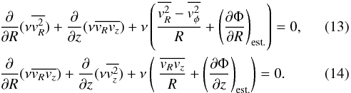 Thus, under the assumption that the approximate integral I3 is exact, Eqs. (13), (14) are used to obtain an estimate of the radial and vertical forces,
 . They can be compared to the exact forces to test the efficiency to recover the galactic potential using our Stäckel integral in a non-Stäckel potential. Figure 6 shows the radial forces KR of the BGM potential and its relative error at several z when recovered from Eqs. (13), (14).
Within the domain R = 3 to 16 kc and z smaller than 3 kpc, the relative error on the radial force KR is smaller than one per cent for R> 6 kpc. The relative error is ten per cent at R = 3 kpc and increases below R = 3 kpc.
Figure 7 shows the exact and recovered Kz force versus z at several R (3.5, 4.5, 6.5, 8.5, 12.5). At large R> 6 kpc, the Kz forces are accurately recovered for the thick disc up to 6 kpc and up to 3 kpc for the thin disc. The vertical force Kz at the solar position R = 8 kpc is remarkably well recovered at 0.5% up to 6 kpc for the thick disc (7 scale heights; Fig. 8). For the thin disc, the accuracy is lost above 3 kpc (corresponding however to ten scale heights of the thin disc). At lower radius R from 3.5 to 5, the Kz force is only approximately recovered up to z = 2 kpc.
For comparison (Fig. 8), we also plot the Kz force recovered neglecting the cross term ⟨ vRvz ⟩ in Jeans equations, a classical assumption valid at low z. We note that this hypothesis remains valid up to 500 pc for the thin disc. At higher z, the recovered force diverges quickly from the exact one.
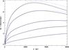 |
Fig. 7 Vertical force Kz versus z at R = (3.5, 4.5, 6.5, 8.5, 12.5 kpc) (top to bottom) from the BGM (black lines) and recovered Kz for a thick disc DF (blue dotted lines). |
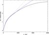 |
Fig. 8 Vertical force Kz versus z at R = 8500 pc (black line) and recovered Kz from simplified Jeans equation assuming the separability of vertical and radial motions: red dotted line for a thin disc DF and blue dashed lines for a thick disc DF. |
5. Collisionless Boltzmann equation
The stationarity of the Jeans equation is a necessary condition for validating the degree of stationarity of a distribution function, but this is not a sufficient condition. We should also have to test the stationarity of all the other moments of the collisionless Boltzmann equation (CBE), since it is easy to find solutions for the Jeans equations that are not solutions of the CBE, so the Jeans equation test can be more optimistic than the indications solely obtained from the conservation of the integral of motion. For this reason we examine hereafter the stationarity of the CBE.
5.1. First estimate
We estimate the stationarity of the distribution function built with the approximated third integral by looking at the time variation of the DF (Eq. (8)) over a dynamical time (~ an orbit revolution). We have ![Mathematical equation: \begin{equation} \label{eq14} \frac{\mathrm d \!\ln f}{\mathrm d t} = \frac{\partial \!\ln f}{\partial t}+\left[ \ln f, H \right] = 0 \end{equation}](/articles/aa/full_html/2015/09/aa26516-15/aa26516-15-eq123.png) (15)or
(15)or  (16)and the relative variation of f over a dynamical or longer time is determined by the variation σI3 of the quasi integral I3 along orbits:
  (17)Orbits with small radial or vertical amplitudes (ΔE and σI3 small) have the smallest variations in f. Thus the thinnest discs are the most accurately modelled.
The stationarity decreases quickly with z since we have  . It also decreases because of the significant presence of resonant orbits between 1 to 2 kpc. However, at the solar Galactic radius R0, orbits within the BGM with large vertical amplitude remain correctly modelled with a Stäckel potential thanks to small σI3 of the order of 0.005. In this situation, the distribution function remains stationary at many scale heights above the galactic plane. For the thick disc, the stationarity (Eq. (17)) is about one per cent at six scale heights (z ~ 6 kpc). For the thin disc, it becomes insufficient at about ten scale heights (z ~ 3 kpc).
The time derivative in Eq. (15) is the time variation from an initial position of stars in phase space at t = 0 given by the initial condition of Eq. (9). How divergent are the orbits evolving from this supposedly near-equilibrium initial condition? We know that for potentials similar to the three potentials considered in this paper, the orbits are essentially regular and an effective third integral must exist, which could be eventually estimated with a higher accuracy using, for instance, high-order polynomials (Bienaymé & Traven 2013) or a torus fitting (Sanders & Binney 2014). This would, however, not be true in cases of significant presence of ergodicity, for instance close to the corotation of a barred rotating potential. It turns out that our approximate integrals oscillate along each orbit around a mean value, that a typical periodicity of these oscillations is the dynamical time, and that the amplitude of these oscillations is of the order of σI3. This is illustrated in Fig. 9 where the maxima of dI3/ dt are of the order of σI3/tdyn with tdyn ~ 6.
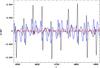 |
Fig. 9 dI3/ dt: time derivative of the quasi integral within the logarithmic potential for the three orbits shown in Fig. 1: (black I3 = 0.16, red I3 = 0.88, blue I3 = 1.06). |
5.2. Second estimate
It is also useful to consider the non-stationarity as a shift in positions or velocities of the modelled DF relative to a stationary DF. A simple 1D dimensional analysis allows it to be illustrated. With a quadratic potential Φ = az2 and a stationary DF as  (18)the shifted DF in velocity by a factor v0 is
 ![Mathematical equation: \begin{equation} f=\exp \left[ -\frac{1}{\sigma^2} \left(\phi(z)+\frac{(v_z-v_0)^2}{2} \right) \right] \cdot \end{equation}](/articles/aa/full_html/2015/09/aa26516-15/aa26516-15-eq140.png) (19)Such a DF could be considered satisfying if the shift is small even if we notice that the relative errors on f increase in the tails of the distribution.
(19)Such a DF could be considered satisfying if the shift is small even if we notice that the relative errors on f increase in the tails of the distribution.
We deduce from the CBE,  (20)which combined with Eq. (17), gives the variation in f over a dynamical time tdyn:
  (21)With a quadratic potential and h, the scale height of the disc population, we estimate the velocity shift:
 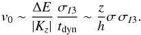 (22)For the thin disc DF at one scale height (h ~ 250 pc), the shift v0 is 0.2 km s-1 and at 4 kpc (16 scale heights), it is 10 km s-1 (to be compared to the 20 km s-1 of the vertical velocity dispersions) where the application of the Jeans equation shows that the DF is not stationary. At one scale height of ~1 kpc for the thick disc, the shift is v0 ~ 1 km s-1. At 6 kpc, it is 7 km s-1 (to be compared to the 40 km s-1 of the vertical velocity dispersion), and the Jeans equation still validates the stationarity.
6. Conclusion
In this paper we have shown that Stäckel potentials can be used to fit a wide variety of disc stellar orbits within different axisymmetric potentials of disc galaxies. We also proposed a new and simple formulation for the third integral of motion of Galactic potentials, explicitly depending on the potential, which is an integral known to be exact in the case of Stäckel potentials.
The quality of the fit of orbits was quantitatively measured by looking at the conservation of the approximate third integral of motion besides the energy and angular momentum. By using the Besançon Galactic model, we showed that the third integral is conserved to a few thousandths in a wide volume around the solar neigbourhood. It is conserved to better than one per cent at 6 kpc above the Galactic plane at the solar position. However, the fit fails at low galactic radius (R smaller than 4 kpc) owing to the presence of a large number of resonant orbits.
In light of the future Gaia data, we also used distribution functions of disc stars, depending on the three integrals, and checked the ability of Jeans equation to recover the gravitational potential. We also considered the stationarity of the CBE.
In conclusion, Stäckel potentials can be good local approximations of general realistic potentials. They have been used many times to fit the global potential of galaxies (see for instance Dejonghe & de Zeeuw 1988) or the potential of our own Galaxy (Famaey & Dejonghe 2003). The fit of stellar orbits are also frequently used using Stäckel potentials with local or global fitting (Kent & de Zeeuw 1991). We showed here that they be can used very efficiently to build distribution function of disc stellar populations. A straightforward application will consist in using such modelling of DFs and in extending the dynamical consistency of the Besançon Galactic model to describe the kinematics of disc stellar populations.
References
- Batsleer, P., & Dejonghe, H. 1994, A&A, 287, 43 [NASA ADS] [Google Scholar]
- Bienaymé, O. 1999, A&A, 341, 86 [NASA ADS] [Google Scholar]
- Bienaymé, O. 2009, A&A, 500, 781 [NASA ADS] [CrossRef] [EDP Sciences] [Google Scholar]
- Bienaymé, O., & Traven, G. 2013, A&A, 549, A89 [NASA ADS] [CrossRef] [EDP Sciences] [Google Scholar]
- Bienaymé, O., Robin, A. C., & Crézé, M. 1987, A&A, 186, 359 [NASA ADS] [Google Scholar]
- Bienaymé, O., Famaey, B., Siebert, A., et al. 2014, A&A, 571, A92 [NASA ADS] [CrossRef] [EDP Sciences] [Google Scholar]
- Binney, J. 2012, MNRAS, 426, 1324 [NASA ADS] [CrossRef] [Google Scholar]
- Colombi, S., Sousbie, T., Peirani, S., Plum, G., & Suto, Y. 2015, MNRAS, in press [arXiv:1504.07337] [Google Scholar]
- Czekaj, M. A., Robin, A. C., Figueras, F., Luri, X., & Haywood, M. 2014, A&A, 564, A102 [NASA ADS] [CrossRef] [EDP Sciences] [Google Scholar]
- De Bruyne, V., Leeuwin, F., & Dejonghe, H. 2000, MNRAS, 311, 297 [NASA ADS] [CrossRef] [Google Scholar]
- Dejonghe, H., & de Zeeuw, T. 1988, ApJ, 333, 90 [NASA ADS] [CrossRef] [Google Scholar]
- de Zeeuw, T. 1985, MNRAS, 216, 273 [NASA ADS] [CrossRef] [Google Scholar]
- de Zeeuw, P. T., & Lynden-Bell, D. 1985, MNRAS, 215, 713 [NASA ADS] [CrossRef] [Google Scholar]
- Famaey, B., & Dejonghe, H. 2003, MNRAS, 340, 752 [NASA ADS] [CrossRef] [Google Scholar]
- Fehlberg, E. 1968, NASA technical report TR R-287 [Google Scholar]
- Hori, G. 1962, PASJ, 14, 353 [NASA ADS] [Google Scholar]
- Kent, S. M., & de Zeeuw, T. 1991, AJ, 102, 1994 [NASA ADS] [CrossRef] [Google Scholar]
- Manabe, S. 1979, PASJ, 31, 369 [NASA ADS] [Google Scholar]
- Lynden-Bell, D. 1962, MNRAS, 124, 95 [NASA ADS] [CrossRef] [Google Scholar]
- Ollongren, A. 1962, Bull. Astron. Inst. Netherlands, 16, 241 [Google Scholar]
- Papaphilippou, Y., & Laskar, J. 1998, A&A, 329, 451 [NASA ADS] [Google Scholar]
- Piffl, T., Binney, J., McMillan, P. J., et al. 2014, MNRAS, 445, 3133 [NASA ADS] [CrossRef] [Google Scholar]
- Renaud, F., Bournaud, F., Emsellem, E., et al. 2013, MNRAS, 436, 1836 [NASA ADS] [CrossRef] [Google Scholar]
- Richstone, D. O. 1980, ApJ, 238, 103 [NASA ADS] [CrossRef] [Google Scholar]
- Robin, A. C., Reylé, C., Derrière, S., & Picaud, S. 2003, A&A, 409, 523 [NASA ADS] [CrossRef] [EDP Sciences] [Google Scholar]
- Sanders, J. L., & Binney, J. 2014, MNRAS, 441, 3284 [NASA ADS] [CrossRef] [Google Scholar]
- Syer, D., & Tremaine, S. 1996, MNRAS, 282, 223 [NASA ADS] [CrossRef] [Google Scholar]
- Valluri, M., & Merritt, D. 1998, ApJ, 506, 686 [NASA ADS] [CrossRef] [Google Scholar]
- van de Hulst, H. C. 1962, Bull. Astron. Inst. Netherlands, 16, 235 [NASA ADS] [Google Scholar]
- Wayman, P. A. 1959, MNRAS, 119, 34 [NASA ADS] [CrossRef] [Google Scholar]
- Yoshikawa, K., Yoshida, N., & Umemura, M. 2013, ApJ, 762, 116 [NASA ADS] [CrossRef] [Google Scholar]
- Zotos, E. E. 2011, New Astron., 16, 391 [NASA ADS] [CrossRef] [Google Scholar]
Appendix A: Quasi integral of motion
We refer the reader to de Zeeuw (1985) and de Zeeuw & Lynden-Bell (1985) for notations and for a detailed description of properties of Stäckel potentials.
An axisymmetric Stäckel potential is fully defined by two free functions h(λ) and
h(ν). In the case of prolate
spheroidal coordinates, ±
z0
( ) are
the foci of the confocal ellipsoids and hyperboloids used to define a system of
coordinates (λ,ν) in which Stäckel potentials are more easily
tractable.
) are
the foci of the confocal ellipsoids and hyperboloids used to define a system of
coordinates (λ,ν) in which Stäckel potentials are more easily
tractable.
Let  be the
true potential that we approximate locally at the position (R1,z1) =
(λ1,ν1) with
a Stäckel potential Φ(λ,ν). We assume that z0 is already
known.
be the
true potential that we approximate locally at the position (R1,z1) =
(λ1,ν1) with
a Stäckel potential Φ(λ,ν). We assume that z0 is already
known.
By definition, we have for a Stäckel potential:
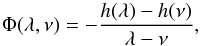 (A.1)and it is always
possible to find a Säckel potential that coincides with any potential on the chosen
coordinate surfaces λ =
λ1 and ν =
ν1. It writes as
(A.1)and it is always
possible to find a Säckel potential that coincides with any potential on the chosen
coordinate surfaces λ =
λ1 and ν =
ν1. It writes as  (A.2)Thus
 (A.3)and
C an
arbitrary constant.
(A.3)and
C an
arbitrary constant.
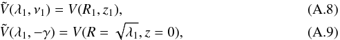
We can express the third integral Is associated to Φ as  (A.4)or
 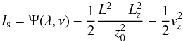 (A.5)with
 (A.6)We fix the
remaining free constant C by setting h(ν = −γ)
= 0, so Ψ
is null at z =
0 in the plane of symmetry of the potential. Then, evaluated at
(λ1,ν1),
this function simplifies as
(A.6)We fix the
remaining free constant C by setting h(ν = −γ)
= 0, so Ψ
is null at z =
0 in the plane of symmetry of the potential. Then, evaluated at
(λ1,ν1),
this function simplifies as 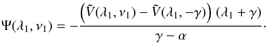 (A.7)If we set
 and
α = 0,
and
α = 0,
 and
and
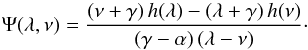
 (A.10)Thus,
from Eqs. (A.4) and (A.7) (similar to Eq. (2)), we obtain a simple expression for the
third integral Is at position (λ1,ν1),
which is exact in the case of a Stäckel potential and explicitly depends on the potential,
the coordinates, and the velocities. We note that, in practice, the intermediate functions
h(λ) and h(ν) do
not need to be evaluated.
(A.10)Thus,
from Eqs. (A.4) and (A.7) (similar to Eq. (2)), we obtain a simple expression for the
third integral Is at position (λ1,ν1),
which is exact in the case of a Stäckel potential and explicitly depends on the potential,
the coordinates, and the velocities. We note that, in practice, the intermediate functions
h(λ) and h(ν) do
not need to be evaluated.
In summary, the proposed quasi integral in Eq. (1) results from the exact third integral of the orbits in the Stäckel potential of Eq. (A.2), which is equal to the true potential on the surfaces λ = λ1 and ν = ν1. The integral is re-evaluated locally for each point (λ,ν) = (λ1,ν1).
The case of Stäckel potentials with oblate spheroidal coordinates leads to the same
equations, but with z0 imaginary,
 and
γ<α. In the z0 = ∞ limit, a
Stäckel potential is separable in R and z,
and
γ<α. In the z0 = ∞ limit, a
Stäckel potential is separable in R and z,  and
and
![Mathematical equation: \appendix \setcounter{section}{1} \begin{eqnarray*} -I_{\rm s}= \left[ V_2(z)-V_2(0) \right] +v_z^2/2 . \end{eqnarray*}](/articles/aa/full_html/2015/09/aa26516-15/aa26516-15-eq180.png) Thus
the vertical energy is an integral of motion.
Thus
the vertical energy is an integral of motion.
In the z0 =
0 limit, Stäckel potentials have the form
 where
r2 =
R2 + z2 and
θ is the
polar angle (Lynden-Bell 1962, Table 1), and the
integral of motion is
where
r2 =
R2 + z2 and
θ is the
polar angle (Lynden-Bell 1962, Table 1), and the
integral of motion is ![Mathematical equation: \appendix \setcounter{section}{1} \begin{eqnarray*} -\,z_0^2 I_{\rm s} \rightarrow [V_2(\theta)-V_2(\pi/2)] +\frac{1}{2}\left(L^2-L_z^2\right) . \end{eqnarray*}](/articles/aa/full_html/2015/09/aa26516-15/aa26516-15-eq185.png)
All Tables
All Figures
|
Fig. 1 Top panel: meridional projection for three orbits within the logarithmic potential (Sect. 3.2) with Lz = 8.5 and ΔE = 0.2. Zero velocity curve and some coordinate curves of the elliptic coordinates (with z0 = 5.9) are drawn. Middle panel: analytical determination of the envelopes of the orbits. Bottom panel: surfaces of section for the same three orbits. Black crosses: numerically computed orbits. Red lines: the corresponding sections obtained from Eqs. (1)−(3). Blue line: surface of section of the orbit confined in the mid-plane (i.e. vz = 0). |
| In the text | |
|
Fig. 2 Left: quasi integral I3 versus zmax for stars with ΔE = 6400 and Rc(Lz) = 8500 pc for the BGM potential. Errors bars are σI3. Right: idem with ΔE = 12 800. |
| In the text | |
|
Fig. 3 Left: dispersion σI3 of the integral I3 along orbits versus zmax for stars with ΔE = 6400 and Rc(Lz) = 8500 for the BGM potential. Right: idem with ΔE = 12 800. |
| In the text | |
|
Fig. 4 BGM potential: z0 best fit versus Rc(Lz) and ΔE. Black lines ΔE = 100 and 200; red lines: 400 and 800; green lines: 1600 and 3200; blue lines: 64 000 and 128 000. |
| In the text | |
|
Fig. 5 Histograms of I3 dispersion along orbits for zmax intervals delimited by 0, 1000 pc, 2000 pc, and beyond (respectively black, dotted red, dashed blue lines). For each of the three zmax intervals, the medians of σI3 are respectively 5 × 10⁻⁴, 1.5 × 10⁻³, and 5 × 10⁻³. |
| In the text | |
|
Fig. 6 Left: dark lines: radial forces KR of the BGM at several z above the galactic plane (0.5, 1, 2, and 3 kpc, bottom to top). Thin green lines: KR recovered from a Jeans equation in the case of a thick disc. Thin red lines: the case of a thin disc. Right: relative errors on the recovered radial force KR versus R at various z (0.5, 1, 2, and 3 kpc; resp. green, black, red, and blue lines) for thin disc DF (dotted lines) and thick disc DF (continuous lines). |
| In the text | |
|
Fig. 7 Vertical force Kz versus z at R = (3.5, 4.5, 6.5, 8.5, 12.5 kpc) (top to bottom) from the BGM (black lines) and recovered Kz for a thick disc DF (blue dotted lines). |
| In the text | |
|
Fig. 8 Vertical force Kz versus z at R = 8500 pc (black line) and recovered Kz from simplified Jeans equation assuming the separability of vertical and radial motions: red dotted line for a thin disc DF and blue dashed lines for a thick disc DF. |
| In the text | |
|
Fig. 9 dI3/ dt: time derivative of the quasi integral within the logarithmic potential for the three orbits shown in Fig. 1: (black I3 = 0.16, red I3 = 0.88, blue I3 = 1.06). |
| In the text | |
Current usage metrics show cumulative count of Article Views (full-text article views including HTML views, PDF and ePub downloads, according to the available data) and Abstracts Views on Vision4Press platform.
Data correspond to usage on the plateform after 2015. The current usage metrics is available 48-96 hours after online publication and is updated daily on week days.
Initial download of the metrics may take a while.