| Issue |
A&A
Volume 581, September 2015
|
|
|---|---|---|
| Article Number | A7 | |
| Number of page(s) | 7 | |
| Section | Planets and planetary systems | |
| DOI | https://doi.org/10.1051/0004-6361/201526346 | |
| Published online | 25 August 2015 | |
Planetary candidates around the pulsating sdB star KIC 5807616 considered doubtful
Mt. Suhora Observatory, Pedagogical University of Cracow,
ul. Podchora¸żych 2,
30-084
Cracow,
Poland
e-mail:
This email address is being protected from spambots. You need JavaScript enabled to view it.
Received: 17 April 2015
Accepted: 12 June 2015
Abstract
Context. It has been suggested that two weak signals observed in the low frequency region of the Fourier transform amplitude spectra from the KIC 5807616 Q5-Q8 data can be interpreted as a result of the light reflection from planets orbiting the host star. Ever since the last results on KIC 5807616 were presented, the Kepler spacecraft has collected over two years of additional data, which we analysed using asteroseismological methods.
Aims. To verify and improve on previous results, we used the Q 5-Q 17 Kepler data to identify pulsational modes, determine multiplet splitting, and to re-analyse the low frequency region between 33−49 μHz where two frequencies, claimed as the planetary signature, were found.
Methods. Since Fourier transform amplitude spectra of the KIC 5807616 data do not show any clear multiplets, we used two stable acoustic modes to determine the theoretical width of gravity mode multiplets and their splittings. The period spacing and histograms of common multiplet component separations were used to identify pulsation modes and the observed gravity mode splittings. In the low frequency region, we analysed the amplitude variations of two planetary signature frequencies over the whole observing run.
Results. We determined the rotational period of the star from the splittings. Analysis of the low frequency region shows that the amplitude and frequency change of the signals found there have similar characteristics to other gravity modes.
Conclusions. New data allow for identifying gravity modes in a limited period range, as well as better rotational period estimations. We suggest that the so-called planetary signature frequencies found in previous work might instead be pulsation modes visible beyond the cut-off frequency of the star.
Key words: subdwarfs / stars: rotation / asteroseismology / planetary systems
© ESO, 2015
1. Introduction
KIC 5807616 is a pulsating B-type hot subdwarf (sdB), also known as KPD 1943+4058, from the extreme horizontal branch of the H–R diagram. Its preliminary Q 2.3 data from the Kepler exploratory phase was initially analysed by Østensen et al. (2010) and Reed et al. (2010), while Van Grootel et al. (2010) derived KIC 5807616’s stellar parameters from spectroscopic observations. The star pulsates in both gravity (g-) and pressure (p-) modes, therefore it is a hybrid sdBV (Schuh et al. 2005; Baran et al. 2005). Its 27 730 ± 270 K effective temperature, log g = 5.52 ± 0.03 surface gravity, and 0.496 ± 0.002M⊙ mass (Van Grootel et al. 2010) are typical of this class of objects.
The following Q 5−Q 8 quarters of KIC 5807616 observing data have been analysed by Charpinet et al. (2011). They find that the star has a rich pulsation spectrum, but only two p-modes and several g-modes (one higher than l = 2) were identified. The reason for the limited success of mode identification was the lack of clear multiplet structures in the Lomb-Scargle periodograms of the KIC 5807616 light curve. Despite having a limited number of multiplets, Charpinet et al. (2011) were able to derive the rotational period of the star as 39.23 days, from the splitting of two p-mode multiplet components. Finally, Charpinet et al. (2011) argue that the weak modulations in the low frequency region can be explained by the existence of planets around KIC 5807616. Using the cut-off frequency (Hansen et al. 1985) to determine the limit for pulsational periods, as well as careful analysis of the light curve, Charpinet et al. (2011) conclude that 5.7625 and 8.2293 h periods visible in their periodogram come from the reflection effect of two planets orbiting KIC 5807616. The analysis of the amplitude ratio of multiplet components allowed them to determine the inclination of the star’s rotational axis to be ~ 65° ± 10° and in this way established the orbital plane inclination of the planetary system.
Since then the Kepler spacecraft has collected eight quarters of KIC 5807616 observing data, and in this work we present the results of the Fourier transform (FT) amplitude spectra analysis of the whole Q 5−Q 17 light curve, as well as of four shorter data sets (seasons). All significant FT signals were also analysed by means of the high resolution (200 days) time-frequency or running FT. We focused on the mode identification, multiplet structures, and the low frequency region, where the signatures of two planetary candidates were claimed. A nearly three times longer set of data allowed us to change some preliminary estimates and to shed new light on the interpretation of planetary signature frequencies.
2. Data and mode identification
During the exploratory phase, KIC 5807616 was observed in the second quarter for one month (Q 2.3) in the short cadence data mode of 58.89 s exposure time and for three months in the long cadence data mode of 30 min exposure time. Following a six month gap, the star has been observed continuously from Q 5 up to Q 17, i.e. until the failure of the second Kepler reaction wheel had occurred. We used this continuous set of short cadence data (1114.5 days or ~3 years) for the FT analysis.
To avoid possible flux contamination by the neighbouring stars in the field, we downloaded the short cadence data target pixel Kepler data from the Barbara A. Mikulski Archive for Space Telescopes (MAST). The fluxes were then extracted only from non-contaminated pixels and preprocessed using cotrending basis vectors (see Kepler Data Release 12 Notes). Points outlying more than 3σ from the running mean of ten points were removed from the data, along with the remaining trends (by fitting spline functions). Since Kepler pixel data before Q 15 suffer a time problem (Kepler Data Release 21 Notes), all data points were accordingly time-corrected. The fluxes were then converted into ppt units (parts per thousand) and used to calculate the FT of the whole light curve and FTs of the seasonal data resulting from the division of the whole 1114 day light curve into four approximately equal (~280 days) parts (seasons 1, 2, 3, and 4). Following standard procedures, the pulsation frequencies were selected from the FTs and simultaneously fitted to the time series data using nonlinear least-squares techniques and prewhitened from the data. The prewhitening process was repeated until most frequencies with a signal above the 4σ detection threshold of 0.01743 ppt (calculated for the whole data within 0−600 μHz) were removed.
For the low frequency region (10−100 μHz) and a couple of frequencies, we also used a local detection threshold of 0.015 ppt. The detection thresholds for seasonal data were 0.037 ppt (calculated between 0−600 μHz where all of the high amplitude modes are present) and 0.023 ppt (above 600 μHz). The frequency resolution calculated as 1.5/T (T − the time span of the data) for Q 5−Q 17 was ~0.01 μHz, allowing for very close frequencies to be fitted. The FT resolutions of any of the seasonal data were better than the 200 days running FTs (0.06 and 0.09 μHz, respectively). Owing to the amplitude, phase, or frequency variations, several of the frequencies could not be prewhitened. Therefore, some of them were manually added later to the fitted frequency list. In total, we were able to fit over 190 frequencies to the light curve of KIC 5807616.
Because the FT of the KIC 5807616 light curve does not show clear multiplet structures, less than half of the fitted frequencies were useful for mode identification. The only two clearly visible multiplets, with well separated and stable components, were found in the p-mode frequency region at 3431.8383 and 3447.2453 μHz. Therefore, for mode identification we used widths and general appearance of the multiplets in the FTs of the whole and seasonal data, as well as in high resolution running FTs calculated within a narrow ±1.7 μHz frequency range around multiplets. In most cases, their internal structure was ignored.
Central frequencies of 56 multiplets used for mode identification in the g-mode frequency region between 89.99−542,17 μHz.
2.1. Period spacing fit
Since there are no clear multiplet structures in the g-mode frequency region, we decided to visually choose central frequency positions of multiplets from the whole data FT, instead of relying on the fit frequencies. Then, we converted them to periods, for the period spacing fit. Because higher modes are expected to be reduced in amplitude by geometric cancellations (Dziembowski 1977), the selection of periods for spacing fits started with the assumption that the largest amplitude periods are l = 1 mode, and the rest were fitted as l = 2 modes. When all high amplitude modes were assigned, we used a deviation criteria. Modes that deviated noticeably from one-mode period spacing were fitted with another set of periods and assigned to the set in which their deviations from the period spacing were smaller. This preliminary assignment of modes was changed afterwards based on a visual inspection of l = 1 and l = 2 multiplet structure splittings and widths. For that purpose, following Charpinet et al. (2011), we determined the theoretical g-mode frequency splittings from two clear p-mode multiplets mentioned earlier (see also chapter Multipletsandrotation below). This way we estimated g-mode splittings equal to 0.129 and 0.215 μHz for l = 1, l = 2 modes, respectively, and used them for mode identification. In Fig. 1 we present final period spacing (ΔP) vs. reduced period (P) diagram for period spacing fits ΔPl = 1 = 241.48 ± 0.26 s and ΔPl = 2 = 139.43 ± 0.15 s. Since the reduced period for l = 1 is  and for l = 2 modes,
  , only l = 2 modes periods were multiplied by
  to avoid large numbers in Fig. 1. Some of the modes can be classified equally well as l = 1 or l = 2 modes. There are also a few modes that could be classified as l = 3, but we lack stronger evidence of that.
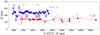 |
Fig. 1 ΔP vs. reduced period (divided by |

Using period spacing one can identify modes between ~2000 and ~12 000 s. For longer periods, the spacing becomes comparable to the width of multiplets, and period spacing fit does not work accurately. For shorter periods the scatter of spacings between consecutive periods varies too much to rely only on the period spacing fit. Therefore, without clear multiplets we could identify only 56 modes (35 l = 1 and 21 l = 2 modes) in a narrow range of periods. Table 1 summarizes our identification efforts. We note that the first period 11111.8 s (89.99421 μHz) in Table 1 identified as l = 2 modes falls below the l = 2 105.69 μHz cut-off frequency of gravity modes determined by Charpinet et al. (2011) (see the discussion of the cut-off frequency in Sect. 4 below). Since most of the fit frequencies can only be used for some statistical purposes (for example an average l = 1 or l = 2 multiplet component splitting determination), we decided to show only those frequencies that correspond to visually determined positions of the multiplet centres. The amplitudes given at these frequencies correspond to the amplitude of the highest peak of a given multiplet visible in the FT of the whole time series data.
In theory, the equal period spacing of gravity modes can be disturbed by mode trapping because of the transition zone between the hydrogen envelope and the helium mantle of the sdBV star (and perhaps by the transition zone between the mantle and the core, Charpinet et al. 2013). The deviations of trapped modes from equal period spacing make ΔP vs. P patterns dependent on the hydrogen mass and in some cases can be used to estimate hydrogen masses of sdBV stars (Krzesinski et al. 2014). However, the analysis of KIC 5807616 ΔP vs. P diagrams in this regard has proved inconclusive.
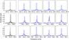 |
Fig. 2 Three highest amplitude l = 1g-modes. Left panels show all data FT, panels on the right present season 1, 2, 3, 4 data FTs. Note the change in amplitudes and multiplet component visibility. Amplitudes are normalized by the maximum amplitude of the all data FT in the left panels and by maximum multiplet component amplitudes occurring during seasonal data in the right panels. |
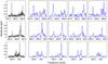 |
Fig. 3 Best examples of l = 2g-modes. None of the multiplets show all multiplet components excited at the same time. Amplitudes are normalized the same way as in Fig. 2. Widths of all panels in Figs. 2 and 3 are the same (1.4 μHz). |
The visibility of m componentes depends on the inclination of the star’s rotation axis (Randall et al. 2005). Assuming that all component intrinsic amplitudes have the same level of excitation, one could use multiplet amplitudes to determine the orientation of the rotation axis in space as done by Charpinet et al. (2011) for KIC 5807616 star. However, hot subdwarfs are not stochastically driven, and the equipartition of energy between multiplet component amplitudes fails (e.g. Pablo et al. 2012, see their Figs. 2 and 5).
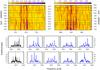 |
Fig. 4 Top panel: 200 days running FT of the whole data near 3431.8383 and 3447.2453 μHz showing amplitude and phase changes of the two p-modes. Both running FT plots have the same width of 3.5 μHz. The two bottom panels show the ordinary FT of the same frequency regions: all data FT (the first panel on the left) and FT of season 1,2,3,4 data (next four panels on the right). Amplitudes were normalized by the largest amplitude of all seasons. |
In Fig. 2 we show the three highest amplitude (according to the frequency and amplitude fits to the whole time series data) l = 1g-modes. Two of them have single peaks visible in their whole data FT, but seasonal FTs in the middle panels of Fig. 2 reveal an unstable triplet structure. More convincing are three examples of the best l = 2g-modes (Fig. 3). Their multiplets do not have full m componentes excited, but at least two components are visible in every one of them. One can note that the excited azimuthal m-orders of these modes are different in each presented mode, which contradicts our expectations coming from linear theory, that m componentes are equally excited. In both Figs. 2 and 3 FTs we can see that most of the multiplet m component amplitudes change greatly: some of them disappear completely, while others grow in amplitude. Taking this into account and having more data to prove it, we show that the average amplitude ratios of any multiplet m componentes will be different for different seasons and will lead to non-consistent conclusions. Therefore, the inclination of the rotation axis of the star cannot be determined this way.
Two clear p-mode component frequencies.
3. Multiplets and rotation
The rotation of a star lifts degeneracy in azimuthal order, creating multiplets. The frequencies of the multiplet components will be separated in the frequency domain following the asymptotic relations:  , for g-modes where Prot is the rotation period and
  is the Ledoux coefficient (Ledoux 1951). For p-modes, the Ledoux coefficient is very small, and multiplet components split into
  frequencies. Since KIC 5807616 pulsates in both p- and g-modes, we can use these relations for mode identification and to determine the stellar rotation rate. Although, in case of KIC 5807616, the task is difficult since in the g-mode frequency region we do not see well-defined multiplets. Instead, we observe rapid seasonal changes in multiplet appearances (Figs. 2 and 3). The FTs of the seasonal data as well as running FTs show constant amplitude and phase change of multiplet components. Because amplitude variation results in generating sidelobes in the frequency domain, while power flow between components manifests as a frequency and phase change, the multiplets split into forests of many frequencies in the final FTs. In this regard g-modes of KIC 5807616 cannot be used in a simple way as a probe of the stellar rotation. However, in the p-mode frequency region, there are two multiplets at 3431.8383 and 3447.2453 μHz (Fig. 4), which were stable for about ~500 days. We identified them as l = 1 and l = 2 modes. Table 2 contains their component frequencies and amplitudes fitted to all and to seasonal data, as well as our multiplet component identifications.
The p-modes show clear multiplets, even in the whole data FT, but to derive their splitting, we used frequencies fitted to the seasonal data (Table 2) and a histogram of the frequency separation between consecutive components of all multiplets vs. separation occurrence numbers. In Fig. 5 we present an averaged sum of ten p-mode splitting histograms, calculated using the bin width of 0.01 μHz and bin centre shifts of 0.001 μHz. The splitting read from the histogram maximum is 0.258 ± 0.006μHz, which is lower then the 0.295 μHz splitting derived earlier by Charpinet et al. (2011).
We also attempted to derive g-mode splittings from similar histograms as described above, but made separately for identified l = 1 and l = 2 modes (Fig. 6). In this case, however, we used frequencies fitted to the whole data instead of the seasonal data. Because g-mode multiplets do not have clear structures, we predicted a theoretical g-mode splitting (assuming solid body rotation) from 0.258 μHz splitting of the two p-modes and estimated the widths of g-mode multiplets. The predicted values of l = 1 and l = 2g-mode splittings are 0.129 and 0.215 μHz respectively. This translates into ~0.258 μHz (for l = 1) and ~0.86 μHz (for l = 2) widths of g-mode multiplets. In Fig. 6 we show histograms of multiplet component frequency separation in broader ranges (top two panels) than predicted multiplet widths to accommodate for possible deviations from predicted values. The bottom panel of Fig. 6 shows the same, but overlapped, histograms (l = 1 black and l = 2 green) presented within the range of l = 1 mode splitting. As one can see, the histograms have weak multiple and scattered maxima. The frequency separation maxima of l = 1 and l = 2 modes are interspersed, which might be caused by wrong mode identification. Although from an eye inspection, we know that some of l = 2 multiplets have additional and closer components than expected for l = 2 modes, therefore, we did not change mode identification based on the histograms.
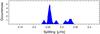 |
Fig. 5 Averaged histogram of p-mode frequency separation based on two multiplets at 3431.8383 and 3447.2453 μHz during seasons 1,2,3, and 4. |
The splitting for l = 1g-modes read from the histogram is 0.106 μHz. For l = 2 modes we have to use an eliminating procedure. For example, the peak at 0.212 μHz (bottom panel of Fig. 6) is very close to double that of the 0.106 μHz splitting, while two separation peaks around 0.1 μHz are likely fake splittings or made by accidently included l = 1 mode into the l = 2 modes sample. The separation peak, which might be considered as a real l = 2 modes splitting is the one at 0.183 μHz. Assuming Ledoux constant (see above) Cl = 1 = 0.5 and Cl = 2 = 0.1667, the theoretical ratio of l = 1 to l = 2 modes frequency splittings should be 0.6. The ratio of the frequency splittings read from our histogram (0.106 / 0.183 = 0.58) is nearly the same as the theoretical one. Both l = 1 and l = 2 mode splittings are lower than 0.129 and 0.215 μHz splittings derived from p-mode multiplets.
Since multiplets are created by the rotation of the star, we can calculate the rotation rate from multiplet frequency splittings. Using the above equations for multiplet splitting and the most reliable 0.258 μHz p-mode splitting, we can determine the rotation period as 44.9 ± 1.1 days. This places KIC 5807616 within slowly rotating sdB stars. The longest, ~90 day rotational period, was recorded for KIC 10670103 (Krzesinski et al. 2014).
Similarly, from g-mode splittings we would have 54.6 ± 4.1 and 52.7 ± 3.2 days rotation rates for l = 1 and l = 2 modes. However, taking multiple maxima of the histograms into account (Fig. 6) and rather weak statistics (we have about 4 occurrences at each histogram maximum out of 56 identified modes e.g.. 35 l = 1 and 21 l = 2 modes) we do not consider g-mode splitting determination to be conclusive.
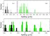 |
Fig. 6 Histogram of l = 1 (top left panel) and l = 2 (top right panel) g-mode frequency separations. The bottom panel shows the enlarged region of the l = 1 histogram overlapped with the histogram of l = 2 modes frequency separations. |
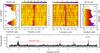 |
Fig. 7 200-day running FTs of the whole data (upper panels) and FT (bottom panel) near two frequencies at 33.839 μHz and 48.182 μHz. Both running FT plots have the same width of 3.5 μHz. Side upper panels show amplitude changes during Q 5−Q 17. Thick dashed lines in the amplitude panels mark the 4σ detection threshold applied in this work (0.01743 ppt), while continuous lines denote the maximum amplitude of background noise near both frequencies. In the bottom panel the dotted line (below the solid one) shows the local detection threshold (0.01549 ppt). |
4. Planets or not planets
In the low frequency range Charpinet et al. (2011) found two frequencies at 33.839 and 48.182 μHz (planetary signature frequencies). After careful analysis of Q 5−Q 8 data and using 61.02 and 105.69 μHz pulsation cut-off limits of l = 1 and l = 2g-modes respectively, Charpinet et al. (2011) interpreted 33.839 and 48.182 μHz peaks in the low frequency region as a result of the light reflected by planets orbiting the KIC 5807616 sdBV star. The observed complex structure around 33.839 μHz was explained as possible evidence of a third body in the system dynamically perturbing the planet at the 33.839 μHz orbital frequency.
Here, using the new Kepler data set we were able to analyse these frequencies and amplitude change over a period of time that is three times longer than the analysis done before and found some problems with previous interpretations of the signals.
Table 3 contains frequencies within 33 – 49 μHz fitted to all and seasonal data, while in Fig. 7 we present high resolution (200 days) running FT windows of 3.5 μHz width around 33.839 and 48.182 μHz and the amplitude variations of these two frequencies during Q 5−Q 17. The signal peak amplitudes for the plot were calculated along the running FT in narrow bands of ±0.4 μHz around the planetary signature frequencies. If more than one peak was found, the amplitude of the highest peak was taken. Similarly, the maximum noise was calculated as the maximum noise out of the noise levels taken from two 0.5 μHz width strips in the proximity of both planetary signature frequencies.
Planetary signature frequency region between 33−49 μHz.
The running FT, as well as the FT of the whole data (bottom part of Fig. 7), shows complex structures around 33.839 and 48.182 μHz frequencies. As already mentioned, similar structures in the frequency domain can be generated by the amplitude and phase changes in the signal, and this is what happens to our planetary signature frequencies (Fig. 7 and Table 3). Both, 33.839 and 48.182 μHz frequencies are not constant in amplitudes, as assumed in the previous work. The peak at 33.839 μHz goes beyond the detection level in the middle of the Kepler run, i.e. after Q 9 (note that Charpinet et al. (2011) analysis only includes Kepler data up to Q 8), while the 48.182 μHz peak goes beyond the detection level at the end of the run. Since one would expect a constant amplitude of the FT signal during the whole observation period, if it is due to the light reflected by the orbiting planets, then change in this amplitude cannot be explained by the reflection effect. In terms of the signal-to-noise ratio, both frequencies have small amplitudes that vary between non-detection (S/N< 4) up to 6 or 8, but the evidence that both amplitudes and frequencies are unstable is convincing. We also note two low amplitude frequencies at 42.3 and 45.2 μHz (see question marks in Fig. 7, asterisks in Table 3), which likely have a similar structure and behaviour to the above planetary signature frequencies, but their S/N is too low to make any certain conclusions. However, if these were signals caused by two additional planets around KIC 5807616, that would raise questions about dynamical stability of the whole close-in planet system.
The Kepler data is known to have an artificial frequency presence (artefacts, Baran 2013) in FTs of the light curves (the list of known artefacts can be found on MAST web pages). If a frequency is found below the pulsation cut-off frequency and is not on the artefact list, we often call it an unknown artefact or we try to find other explanations for its existence. However, the cut-off frequency formula given by Hansen et al. (1985) was derived for white dwarfs and involved some approximations.
For example, the pulsation cut-off frequencies derived for an Eddington grey atmosphere (Hansen et al. 1985, Eqs. (8a) and (8b)) depend on the mean molecular weight μ, log g, and on the effective temperature of the star. If one assumes for the KIC 5807616 sdBV star the same mean molecular weight as for white dwarfs (μ = 1), the l = 1 and l = 2 mode cut-off frequencies will be at 31.28 and 54.18 μHz, respectively. This is about half the 61.02 and 105.69 μHz limits derived by Charpinet et al. (2011), and allows for both planetary signature frequencies to be identified as pulsating g-modes. Decreasing the mean molecular weight down to 0.6 will raise the cut-off frequencies up to ~40 and ~70 μHz. Therefore, final result strongly depends on the assumptions made to derive the cut-off frequencies for stars other than white dwarfs.
We might also need to reconsider our approach to the strict limits of the cut-off frequency, because damping does not necessarily mean that pulsations have to stop beyond it. It simply means that the amplitude of pulsation will be lower and might be difficult to detect. This could be the case for KIC 5807616 (and a couple of other stars), where a few frequencies were detected below the cut-off frequency. They were not found on the list of known Kepler spacecraft artefacts, and we argue they are not planetary signatures either. Therefore, we postulate these are simply pulsation frequencies, which are damped and of low amplitudes, but observed below the cut-off frequency.
5. Conclusions
We performed the analysis of the whole Q 5–Q 17 Kepler data of the KIC 5807616 sdBV star by means of the FTs and high resolution running FTs of its light curve. The FTs do not show clear multiplets in the g-mode frequency region. There are only a few multiplets that have more than one component that is excited and stable for longer periods of time. Therefore, in spite of a large number (~191) of frequencies fitted to the star light curve, we were able to identify only 56 pulsation g-modes (35 l = 1 and 21 l = 2 modes) in a narrow 2000−12 000 s period range (Table 1).
The lack of clear multiplets also makes our identification less reliable.
In the p-mode frequency region, we found two clear multiplet structures that were identified as acoustic l = 1 and l = 2 modes. These were used to derive a 44.9 ± 1.1 days rotation rate of the star envelope/surface, which is five days longer than previous estimates by Charpinet et al. (2011). From the analysis of g-mode splitting, the rotation rate seems to be about ten days longer, suggesting different surface and interior rotation rates. However, our g-mode multiplet-splitting determination is not reliable so this value has to be used carefully.
Finally, we used frequency splittings and amplitude variations of the two 33.839 and 48.182 μHz frequencies to challenge the interpretation that these signals are from planets around KIC 5807616. We also suggest that the pulsation cut-off frequencies should not be treated as strict limits below which one cannot observe pulsating modes. Pulsations might be strongly damped but still visible in the FTs of the light curve. Since the Kepler data were carefully reduced and there are no known artefact frequencies within this region, we concluded that both planetary signature frequencies (and perhaps a couple of others) observed beyond the cut-off frequency limits are most likely of pulsation origin. The example of KIC 5807616 also has implications for other claims of extreme planetary systems around sdB stars based on similar assumptions of the strict cut-off frequency limits for the pulsating modes (Silvotti et al. 2014, KIC 10001893 sdBV), which might need to be reanalysed in a similar way to how it has been done in this paper.
Acknowledgments
This project was supported by Polish National Science Centre grant 2011/03/D/ST9/01914.
References
- Baran, A. S. 2013, Acta Astron., 63, 203 [NASA ADS] [Google Scholar]
- Baran, A. S., Pigulski, A., Kozieł, D., et al. 2005, MNRAS, 360, 737 [NASA ADS] [CrossRef] [Google Scholar]
- Charpinet, S., Fontaine, G., Brassard, P., et al. 2011, Nature, 480, 496 [NASA ADS] [CrossRef] [PubMed] [Google Scholar]
- Charpinet, S., Van Grootel, V., Brassard, P., et al. 2013, EPJ Web of Conferences, 43, 4005 [CrossRef] [EDP Sciences] [Google Scholar]
- Dziembowski, W. 1977, Acta Astron., 27, 1 [NASA ADS] [Google Scholar]
- Hansen, C. J., Winget, D. E., & Kawaler, S. D. 1985, ApJ, 297, 544 [NASA ADS] [CrossRef] [Google Scholar]
- Krzesinski, J., Blokesz, A., Baran, A. S., & Bachulski, S. 2014, Acta Astron., 64, 151 [NASA ADS] [Google Scholar]
- Ledoux, P. 1951, ApJ, 114, 373 [NASA ADS] [CrossRef] [Google Scholar]
- Østensen, R. H., Silvotti, R., Charpinet, S., et al. 2010, MNRAS, 409, 1470 [NASA ADS] [CrossRef] [Google Scholar]
- Pablo, H., Kawaler, S. D., Reed, M. D., et al. 2012, MNRAS, 422, 1343 [NASA ADS] [CrossRef] [Google Scholar]
- Randall, S. K., Fontaine, G., Brassard, P., & Bergeron, P. 2005, ApJS, 161, 456 [NASA ADS] [CrossRef] [Google Scholar]
- Reed, M. D., Kawaler, S. D., Østensen, R. H., et al. 2010, MNRAS, 409, 1496 [Google Scholar]
- Schuh, S., Huber, J., Green, E. M., et al. 2005, ASP Conf. Ser., 334, 530 [NASA ADS] [Google Scholar]
- Silvotti, R., Charpinet, S., Green, E., et al. 2014, A&A, 570, A130 [NASA ADS] [CrossRef] [EDP Sciences] [Google Scholar]
- Van Grootel, V., Green, E. M., Randall, S. K., et al. 2010, ApJ, 718, L97 [NASA ADS] [CrossRef] [EDP Sciences] [Google Scholar]
All Tables
Central frequencies of 56 multiplets used for mode identification in the g-mode frequency region between 89.99−542,17 μHz.
All Figures
|
Fig. 1 ΔP vs. reduced period (divided by |
| In the text | |
|
Fig. 2 Three highest amplitude l = 1g-modes. Left panels show all data FT, panels on the right present season 1, 2, 3, 4 data FTs. Note the change in amplitudes and multiplet component visibility. Amplitudes are normalized by the maximum amplitude of the all data FT in the left panels and by maximum multiplet component amplitudes occurring during seasonal data in the right panels. |
| In the text | |
|
Fig. 3 Best examples of l = 2g-modes. None of the multiplets show all multiplet components excited at the same time. Amplitudes are normalized the same way as in Fig. 2. Widths of all panels in Figs. 2 and 3 are the same (1.4 μHz). |
| In the text | |
|
Fig. 4 Top panel: 200 days running FT of the whole data near 3431.8383 and 3447.2453 μHz showing amplitude and phase changes of the two p-modes. Both running FT plots have the same width of 3.5 μHz. The two bottom panels show the ordinary FT of the same frequency regions: all data FT (the first panel on the left) and FT of season 1,2,3,4 data (next four panels on the right). Amplitudes were normalized by the largest amplitude of all seasons. |
| In the text | |
|
Fig. 5 Averaged histogram of p-mode frequency separation based on two multiplets at 3431.8383 and 3447.2453 μHz during seasons 1,2,3, and 4. |
| In the text | |
|
Fig. 6 Histogram of l = 1 (top left panel) and l = 2 (top right panel) g-mode frequency separations. The bottom panel shows the enlarged region of the l = 1 histogram overlapped with the histogram of l = 2 modes frequency separations. |
| In the text | |
|
Fig. 7 200-day running FTs of the whole data (upper panels) and FT (bottom panel) near two frequencies at 33.839 μHz and 48.182 μHz. Both running FT plots have the same width of 3.5 μHz. Side upper panels show amplitude changes during Q 5−Q 17. Thick dashed lines in the amplitude panels mark the 4σ detection threshold applied in this work (0.01743 ppt), while continuous lines denote the maximum amplitude of background noise near both frequencies. In the bottom panel the dotted line (below the solid one) shows the local detection threshold (0.01549 ppt). |
| In the text | |
Current usage metrics show cumulative count of Article Views (full-text article views including HTML views, PDF and ePub downloads, according to the available data) and Abstracts Views on Vision4Press platform.
Data correspond to usage on the plateform after 2015. The current usage metrics is available 48-96 hours after online publication and is updated daily on week days.
Initial download of the metrics may take a while.