| Issue |
A&A
Volume 581, September 2015
|
|
|---|---|---|
| Article Number | A50 | |
| Number of page(s) | 10 | |
| Section | Extragalactic astronomy | |
| DOI | https://doi.org/10.1051/0004-6361/201526226 | |
| Published online | 02 September 2015 | |
A study on the multicolour evolution of red-sequence galaxy populations: insights from hydrodynamical simulations and semi-analytical models
1 Purple Mountain Observatory, Partner Group of MPI for Astronomy, Chinese Academy of Sciences, 2 Beijing XiLu, 210008 Nanjing PR China
e-mail: This email address is being protected from spambots. You need JavaScript enabled to view it.
2 Excellence Cluster Universe, Technische Universität München, Boltzmannstrasse 2, 85748 Garching, Germany
3 Dark Cosmology Centre, Niels Bohr Institute, University of Copenhagen, Juliane Maries Vej 30, 2100 Copenhagen, Denmark
4 INAF–Osservatorio Astronomico di Roma, via Frascati 33, 00040 Monteporzio Catone, Italy
5 Max-Planck-Institut für extraterrestrische Physik (MPE), Postfach 1312, Giessenbachstr., 85741 Garching, Germany
6 INAF–Osservatorio Astronomico di Capodimonte, salita Moiariello 16, 80131 Napoli, Italy
7 INAF–Osservatorio Astrofisico di Catania, via S.Sofia 78, 95123 Catania, Italy
8 Departamento de Ciencias Fisicas, Universidad Andres Bello, Av. Republica 220, Santiago, Chile
Received: 30 March 2015
Accepted: 1 July 2015
Abstract
Context. By means of our own cosmological-hydrodynamical simulation (SIM) and semi-analytical model (SAM), we studied galaxy population properties in clusters and groups, spanning over ten different bands from the ultraviolet to the near-infrared (NIR), and their evolution since redshift z = 2.
Aims. We compare our results in terms of red/blue galaxy fractions and of the luminous-to-faint ratio (LFR) on the red sequence (RS) with recent observational data reaching beyond z = 1.5.
Methods. Different selection criteria were tested to retrieve the galaxies that effectively belong to the RS: either by their quiescence degree measured from their specific star formation rate (sSFR; the so-called “dead sequence”), or by their position in a colour–colour plane, which is also a function of sSFR. In both cases, the colour cut and the lower limit magnitude thresholds were let to evolve with redshift so that they would follow the natural shift of the characteristic luminosity in the luminosity function (LF).
Results. We find that the Butcher-Oemler effect is wavelength-dependent, with the fraction of blue galaxies increasing more steeply in optical-optical than in NIR-optical colours. Moreover, a steep trend in the blue fraction can only be reproduced when an optically fixed luminosity-selected sample is chosen, while the trend flattens when selecting samples by stellar mass or by an evolving magnitude limit. We also find that the RS-LFR behaviour, highly debated in the literature, is strongly dependent on the galaxy selection function: in particular, the very mild evolution that is recovered when using a mass-selected galaxy sample agrees with values reported for some of the highest redshift-confirmed (proto)clusters. For differences that are attributable to environments, we find that normal groups and (to a lesser extent) cluster outskirts present the highest values of both the star-forming fraction and LFR at low z, while fossil groups and cluster cores have the lowest values: this separation among groups begins after z ~ 0.5, while at earlier epochs all groups share similar star-forming properties.
Conclusions. Our results support a picture where star formation is still active in SIM galaxies at redshift 2, in contrast with SAM galaxies, which have formed earlier and are already quiescent in cluster cores at that epoch. Over the whole interval considered, we also find that the more massive RS galaxies from the mass-selected sample grow their stellar mass at a higher rate than less massive ones. On the other hand, no dearth of red dwarfs is reported at z ≳ 1 from either model.
Key words: methods: numerical / galaxies: clusters: general / galaxies: evolution / galaxies: formation / galaxies: star formation / galaxies: statistics
© ESO, 2015
1. Introduction
The red or blue fraction and the giant-to-dwarf (or luminous-to-faint) ratio are common proxies that contribute to characterize two fundamental properties of the galaxy populations in clusters or groups: the red sequence (RS) of early-type (ET) galaxies in the colour–magnitude plane, and the luminosity function (LF). As to the latter, its characteristic luminosity L∗ is usually taken as a measure of the mean luminosity of giant galaxies, while its slope measures the relative abundance of dwarf galaxies. The variation of these two parameters with redshift and environment allows estimating the growth of the two populations, either in terms of stellar mass or light. In particular, the LF of RS galaxies (RSLF) has been extensively studied, based on which a deficit of faint red galaxies at z ~ 1 and beyond has been reported, both in optical and in redder colours (De Lucia et al. 2007; Krick et al. 2008; Gilbank et al. 2008; Stott et al. 2009; Hilton et al. 2009): this would imply that less massive galaxies undergo a slower evolution inasmuch as their star-forming activity lasts longer than that of more massive galaxies. Nevertheless, works by Andreon (e.g. 2008, 2014) and Crawford et al. (2009) point in the opposite direction, highlighting a non-evolution of the faint-end slope of the LF. The dependence of the latter on environmental and evolutionary parameters is still debated, as is the presence of an upturn at faint magnitudes (see Zucca et al. 2009; Bañados et al. 2010; de Filippis et al. 2011). The controversy is complicated by the fact that different filters, apertures and limiting magnitudes are used in the literature (see Sect. 3). In this respect, stellar mass-based surveys better allow studying the evolution of galaxy populations independently of colours and magnitudes, providing a more straightforward parallel to theoretical models: recently, a study on field galaxies by Tomczak et al. (2014) measured a steepening in the slope of the galaxy stellar mass function at its low-mass end, with an upturn at masses <1010 M⊙ extending to z = 2 and beyond.
On the other hand, the red or the blue fractions are directly connected to the slope and scatter of the RS, which in turn provide relevant constraints upon the epoch and duration of the star formation in ETGs. In fact, the RS itself is also shaped according to changes in the specific star formation rate (sSFR) of member galaxies, as they move from a previously populated blue cloud. Romeo et al. (2008) showed that the epoch at which the switch between the star-forming and the passive regime occurs closely mirrors the epoch at which the RS slope becomes null, that is also when its scatter becomes that of the pure quiescent population. This epoch of migration towards the RS and subsequent passive reddening coincides then with shutting off of the bulk of SF: this may in turn be determined by environmental input such as (gas-poor) mergers between galaxies or by a natural mass threshold set up by internal sources hindering the cold phase condensation, such as energy feedback from AGN (see Cattaneo et al. 2008). The role of AGN feedback helps preventing the cooling of hot gas around massive galaxies, and the subsequent formation of a new disc. Nevertheless, Kang et al. (2007) have suggested that high- and low-mass ETGs formed out of dry and wet mergers, respectively, independent of the presence of an AGN. A comprehensive analysis carried out by Peng et al. (2010) that later was extended by Raichoor & Andreon (2012b), demonstrated that the red or blue fraction is a composite yet separable function of redshift, environment (as measured by the cluster-centric distance in clusters, or by the galaxy density in general), and galaxy stellar mass as well, leading to two quenching modes that act as independently: one driven by environment and another by galaxy mass, only the latter of which is dependent on redshift.
The matter of star formation at high redshift is widely studied in clusters that nonetheless suffer from some selection bias: this occurs for example when they are selected by means of the red sequence itself, which then becomes a premise a priori rather than a diagnostic tool; the opposite may happen in the field, where blue bright galaxies are more likely to be detected at high redshift. Many surveys have measured a significant growth in mass of the RS since z ~ 1 (e.g. Gladders et al. 1998; Bell et al. 2004; Mei et al. 2009), generally basing their results on U- to I-centered filters. On the other hand, Bundy et al. (2005), among others, have found little evolution in the distribution of massive galaxies since z ~ 1 to the present, using the K-band to constrain the stellar mass. Lidman et al. (2008) studied one cluster at z = 1.4 in J − K, finding an already well-defined RS in the core, with a scatter in colours around 0.055, whereas galaxies in the outskirts appear younger and bluer, half of them with high SFR ongoing. More recently, Fassbender et al. (2014) measured a bright end of the LF still evolving at z ≃ 1.6, with a very active ongoing mass-assembly and clear merger signatures for the most massive galaxies, along with an RS well populated at magnitudes fainter than  , but still lacking bright objects above it. A significant population of massive galaxies much bluer than the RS was also detected by Strazzullo et al. (2013), who probed the massive-end galaxies in a proto-cluster core at z = 2, finding therein a mixture of both quiescent and star-forming galaxies. Contrasting results from Raichoor & Andreon (2012a), Andreon et al. (2014), and Newman et al. (2014) indicate instead that all most massive core galaxies are already red and passive in a proto-cluster spectroscopically confirmed between z = 2.2 and 1.8, having a deep completeness in galaxy mass.
As a widespread manifestation of the scenario above, the Butcher-Oemler (BO) effect (Butcher & Oemler 1984 = BO84) implies that clusters at higher redshifts have a higher fraction fbl = Nblue/Ntot of blue galaxies. Since that pioneer photometric work, which was valid up to z = 0.6, galaxy infall has been put forward as a likely mechanism for increasing the blue fraction in intermediate-redshift clusters (e.g. Kauffmann 1995; Couch et al. 1998; van Dokkum et al. 1998; Ellingson et al. 2001; Fairley et al. 2002). A time-declining blue fraction in the hierarchical framework is a natural consequence of environmental suppression of star formation in over-dense systems (see Diaferio et al. 2001), whereby the transition from blue to red regimes occurs first and mainly outside the cluster core in response to processes such as ram pressure stripping, galaxy encounters, or strangulation (e.g. Berrier et al. 2009). Evidence that the RS scatter was still tight at higher redshift (e.g. Ellis et al. 1997, at z = 0.55; Stanford et al. 1998, at z = 0.9) implies a homogeneity of the ET population across cosmic time, which is in contrast with the strong evolution of the cluster galaxies predicted by some interpretations of the BO effect. The latter can be interpreted by means of the transformation of blue field galaxies into red cluster ones, but only if such infall is accompanied by a morphological change from spirals to ETs (or an equivalent change from star-forming to passive), then the scatter of the colour–magnitude relation is expected to increase as a result of the higher number of blue ETs approaching the RS (see Schawinski et al. 2014; Cen 2014). Moreover, a recent (z< 1.3) transformation of many blue galaxies into faint red ones would modify the faint-end slope of the LF itself and again increase the RS scatter to an extent that is not observed at that epoch (see Andreon 2008).
Thus the evidence of the BO effect is under many aspects still controversial because of discrepancies in the sample selections (waveband, completeness limit, cluster dynamics) and defining criteria for a red colour threshold. Selection of galaxy samples in the near-infrared as opposed to the optical should result in samples more representative by stellar mass (Aragón-Salamanca et al. 1993; Gavazzi et al. 1996) because near-infrared (NIR) or mid-infrared (MIR) colours are almost insensitive to star formation histories. Given that luminosities and colours of galaxies selected in the K-band more reliably trace their behaviour in terms of stellar mass, K-selected samples can be used to constrain the masses of the blue galaxies in excess at high z, which are thought to evolve into S0 galaxies or dwarfs later on (De Propris et al. 2003). In fact, Haines et al. (2009) found that the star-forming fraction in J − K follows a fairly mild evolution at 0 <z< 0.4, which becomes constant at around 50% if considering only the innermost galaxies within R500; this indicates that the residual BO effect would be entirely due to the infall galaxies in the outer cluster regions.
In this paper we model the global properties of the ET galaxies assembly and evolution in over-dense regions by means of cosmological and hydrodynamical simulations (hereafter SIM) that include chemical evolution, and with the independent aid of a novel semi-analytical model (SAM) – that are both described in Sect. 2. This is pursued by reproducing the evolution of the RS luminous-to-faint ratio (LFR) and the blue fraction, as complementary yet independent means of diagnostics. To shed light upon the combined mechanisms that are at the base of the regularity in the global properties of the ET populations in clusters and groups, one important step is choosing reasonable criteria for defining a correspondence between the observed RS and a subsample of ET galaxies descending from the models that, by their ages and metallicities, can be safely considered as belonging to the RS: this task is detailed in Sect. 3. The motivation behind the choice of our diverse model sets is then to assess how the different methodologies with respect to observational data affect our results, as well as to investigate their dependence on the physical processes implemented in either model.
2. Methods
2.1. Simulations
The formation of our galaxies is followed ab initio within a 150 Mpc cosmological volume, which allows accounting for their interaction with a large-scale environment. The initial N-body simulation adopts a standard Λ cold dark mater cosmology, with ΩΛ = 0.7, Ωm = 0.3, Ωb = 0.045, h = 0.7, and σ8 = 0.9. This simulation serves as input for the volume re-normalization technique to achieve higher resolution in zoomed regions such as individual clusters and groups, which are later re-simulated with the full hydrodynamical code (see Romeo et al. 2006). Thus the mutual cycle between intergalactic medium (IGM), star formation (SF) and stellar feedback can be described in a self-consistent way at the cluster scale by means of the baryonic physics implemented in the hydrodynamical code: this includes a metal-dependent radiative cooling function (with cooling shut-off below 104 K), thermal conductivity, star formation according to a top-heavy initial mass function (IMF), chemical evolution with not-instantaneous recycling, feedback from supernovae (SN)-Ia and SN-II, and SN-II-driven galactic winds. The whole cycle of gas-stars follows the birth and evolution of the star particles and their final decay again into gas particles through a feedback mechanism; the latter in turn regulates further episodes of SF, and so forth.
By re-zooming on target-selected regions at higher resolution, we were able to resolve down to galaxy-sized haloes and model their stellar populations: a mass resolution of stellar and gas particles down to to 3 × 10⁷h-1 M⊙ was achieved in this way. In particular, the virial mass of the haloes selected at z = 0 to be re-simulated at higher resolution are 1 × 10¹⁴ M⊙ for groups, 3 × 10¹⁴ M⊙ for the lower mass cluster and 1.2 × 10¹⁵ M⊙ for the larger one - measured within the virial radius defined as enclosing an over-density of 200 times the critical background density. Out of the 12 re-simulated groups at z = 0, four were of fossil nature (see D’Onghia et al. 2005). Galaxies from homogeneous density regions were stacked together to make up four environmental classes: cluster cores (IN), cluster outskirts (OUT), normal groups (NG) and fossil groups (FG); the separation between these cluster regions is given by one-third of R200.
In the SPH scheme, each star particle represents a single stellar population (SSP) of total mass corresponding to the stellar mass resolution of the simulation. The individual galaxies are assigned a luminosity as the sum of the luminosities of its constituent star particles in the broad bands UBVRIJHK (Johnson/Cousins filter, Vega system). The individual stellar masses are distributed according to an Arimoto-Yoshi (AY) IMF; each of these SSPs is characterized by its age and metallicity, from which luminosities are computed by mass-weighted integration of the Padova isochrones (Girardi et al. 2002). Thus the physically meaningful quantities of our data are age and metallicity, from which colours are derived. Results from this approach have already involved the study of global galaxy properties such as the RS (Romeo et al. 2005, 2008) and the mass-metallicity-SFR relations (Romeo Velonà et al. 2013).
2.2. SAM
The SAM used in this paper is based on Kang et al. (2005), which later was developed in Kang et al. (2012), and to which we refer for details. The main ingredients are hereby introduced as follows. The simulation was performed using the Gadget-2 code (Springel 2005) with cosmological parameters adopted from the WMAP7 data release (Komatsu et al. 2011), namely: ΩΛ = 0.73, Ωm = 0.27, Ωb = 0.044, h = 0.7 and σ8 = 0.81; the cosmological box had a size of 200 Mpc/h on each side and was populated with 10243 particles. The merger trees are constructed by following the subhaloes resolved (by using SubFind: Springel et al. 2001) in friends-of-friends (FOF) haloes at each snapshot. The SAM is then grafted on the merger trees and self-consistently models the physics processes governing galaxy formation, such as gas cooling, star formation, supernova, and AGN feedback. Finally, the galaxy luminosity and colours are calculated based on the stellar population synthesis of Bruzual & Charlot (2003) adopting a Chabrier stellar IMF (Chabrier 2003).
In particular, the SAM includes radio-mode AGN feedback, parametrized in a phenomenological way as in Croton et al. (2006). This mechanism works so as to suppress the cooling in massive haloes, whose star formation in the central galaxies is hence shut off, drifting them onto the RS. In the present model, developed in Kang et al. (2006), the heating efficiency of the surrounding gas is proportional to a power of the virial velocity of the host halo, hence the gas cooling continues to form stars until a massive spheroid forms at the galaxy centre. In this way, more massive and luminous galaxies can be formed at high redshift, thus achieving a successful reproduction of the observed LF in rest-frame K-band and the galaxy colour distributions.
Moreover, it is worth briefly discussing here the treatment of gas stripping from dwarfs/satellites in the model. In this regard, a common outcome of most SAMs has been the overabundance of red faint galaxies produced, which has generally been ascribed to the low efficiency in tidal disruption of dwarfs tout court (see Weinmann et al. 2011) and at the same time to a too efficient ram-pressure stripping of those that survived. In particular, most SAMs assume that the entire hot gas reservoir of a galaxy is instantaneously stripped at the very event of accretion into a larger halo, that is, inmediately after infall when it becomes a satellite. In our model we instead let the outer hot gas in dwarfs be gradually stripped over a timescale of about 3 Gyr: this prolonged strangulation results in a longer-lasting cooling and hence delayed quenching of SF. As demonstrated in Kang & van den Bosch (2008), this recipe can effectively lower the dwarf fraction on the RS and, if combined with a stronger tidal disruption prior to the central accretion, can fairly well reproduce the observed RSLF without affecting its bright end. Finally, in our SAM there is no ram-pressure stripping of cold gas from the host halo (a mechanism leading to the so-called starvation), which means that this inner component is normally consumed by star formation and SN feedback.
From the initial simulation box, a total number of haloes above the threshold of 1 × 10¹⁴ M⊙ were extracted, ranging from 2830 (z = 0) to 2150 (z = 0.5), 1300 (z = 1), down to 300 (z = 2); out of these, those below 1.5 × 10¹⁴ M⊙ were classified as groups. Finally, and relying on Menci et al. (2008), we note that the different normalization of the power spectrum assumed in our models, although affecting the cluster abundance at a given redshift, is not effective in changing the dynamical history of DM haloes, nor their stellar mass assembly. The colour output of galaxies and the luminosity function are instead more prone to be affected by different choices of the IMF (see Romeo et al. 2008), even though both our options are top-heavy.
3. Definition of RS samples
All models have to undergo substantial difficulties when directly compared with observations: first, galaxy spectral energy distributions (SEDs) are often only poorly sampled with the current bands, especially at high z, therefore any attempt to convert to rest-frame colours would introduce a large systematic error in these cases. Secondly, when considering the stellar masses, the dominant systematic error comes from the choice of the IMF, which gives a factor two uncertainty in the LFR results and is most likely the main source of scatter in the compilation of different data from literature; our Arimoto-Yoshii IMF in the SIM produces stellar masses between a Chabrier and a Salpeter IMF, which are commonly used for the conversion. Third, all background-subtracted quantities are measured within a cluster-centric radius that is quite small in the high-z cases to provide the highest signal-to-noise ratio (for example the 30′′ aperture corresponds to 255 kpc in the z = 1.58 cluster of Fassbender et al. 2014). Therefore they can be consistently only compared with our cluster core points. Finally, clusters themselves compose an utterly heterogeneous family, and many features of galaxy populations may partially depend on correlations between cluster and galaxy properties, such as cluster mass and dynamical state: high-z surveys are generally biased towards richer clusters, which are more dynamically evolved. This in turn will affect galaxy colours and star formation histories; evidence of this is that lower galaxy blue fractions are measured when including X-ray selected clusters, which are on average more massive and relaxed (see Andreon & Ettori 1999).
Throughout the following analysis we refer to galaxy samples excluding the BCG. All model apertures are differential, being fixed to the virial radius at each epoch: this naturally accounts for the cluster cosmic evolution and leads to some extent to a blue segregation outside the cluster cores (see Ellingson et al. 2001).
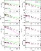 |
Fig. 1 Redshift evolution of the mean rest-frame colours of the DS samples from the SIM: clusters IN (black rhombi), clusters OUT (open circles), normal groups (blue triangles), fossil groups (red squares); and from the SAM (green): clusters IN (dashed lines), clusters OUT (dotted lines), and groups (dot-dashed lines). It is also indicated the difference in colour during the redshift interval: |

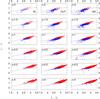 |
Fig. 2 Double-colour diagrams for galaxies more massive than 3 × 10⁹ M⊙, selected by their specific SFR: higher (blue) and lower (red) than 10-11/yr; larger symbols are for SIM, dots for the SAM. Solid lines are given by the fitting formulae that separate the two regions: U − V = 0.5(V − K) − 0.5 for 0 ≤ z< 1, U − V = 0.5(V − K) − 0.6 for 1 ≤ z ≤ 1.5, U − V = 0.45(V − K) − 0.54 for 1.5 <z ≤ 2. |
We define the dead-sequence (DS) sample to be the sample of galaxies with no star formation ongoing over the last Gyr, and plot in Fig. 1 its average colours as a function of z in different wavebands, motivated by the LF of RS galaxies being strongly dependent on the latter, as stated for example by Goto et al. (2005). As a general trend, differences among the four environments are scarce in absolute value; they are more evident in U − V, B − V, and U − R: the reddest colour in any band and at every z is presented by cluster core galaxies, while normal groups have the bluest colours on average. This is in line with the environmental sequence found in R08, where normal groups were characterized by intrinsically higher SFR than FGs. It also confirms that at the opposite end, galaxies in denser cluster cores are redder. Differences between SIM and SAM show that the latter yields a redder colour distribution at any epoch, and especially in V − K: this is expected, since most SAMs are producing too many galaxies whose stellar mass bulk was formed too early (see Discussion). The redshift evolution appears to strongly depend on the wavelength: the steepest reddening in time is observed in the five colours within UBVR bands, where it amounts to one-third with respect to the present colour on average; and especially in U − B, where the difference peaks at about half of this value, in stark contrast with suggestions by Willmer et al. (2006) for clusters at z ~ 1. On the other hand, it is much flatter in V − I and V − K and is almost exactly constant (at a value below 1) in J − K. The latter are also those where the least difference is noted among environments. This confirms that measures of optical-optical colours are strongly affected by recent episodes of star formation, whereas optical-NIR colours are mostly sensitive to intrinsic changes in metallicity and stellar mass. We use these mean colours (shifted 0.2 mag bluewards) in the following to select the RS samples as our first criterion. This reproduces the original definition chosen by BO84, where cluster galaxies bluer than 0.2 mag in B − V with respect to the RS ridge were selected. It is worth stressing that the threshold yielded by this criterion naturally evolves with z: this procedure is equivalent to that of Andreon et al. (2006), who instead adopted an evolving colour cut Δ(B − V) below a fixed RS upper limit. It is also consistent with the method of Raichoor & Andreon (2012b), who assumed a synthetic model from Bruzual & Charlot (2003) computed for solar metallicity, formation redshift of zf = 5, and an exponentially declining star formation history ∝exp( − t/τ) with τ = 3.7 Gyr as a divisory line for a red classification at any redshift (shown in Fig. 1 as reference in the U − R panel).
In Fig. 2 our galaxies are plotted within a particular colour–colour plane that has been proven to efficiently distinguish between quiescent and star-forming galaxies up to z ~ 2 (see Williams et al. 2009). When the two populations are classified according to their specific SFR (sSFR), this bi-colour plot allows separating them by means of simple diagonals that are almost unchanged over the whole redshift interval. This can provide an alternative selection criterion for defining the two samples: from our joint SIM+SAM distribution, U − V = α(V − K) − β is best fitted by the values (α,β) = (0.5,0.5),(0.5,0.6),and(0.45,0.54) for z = 0 − 1, z = 1 − 1.5, and z = 2, respectively.
We also checked for alternative criteria to define the RS samples and computed the U − V and U − B blue fractions following the empirical thresholds given in Bell et al. (2004) and Willmer et al. (2006), respectively, which hold for z ≤ 1:  These colour cuts were modified as luminosity-dependent to avoid excluding faint RS galaxies due to the very slope of the RS (see Crawford et al. 2009).
Moreover, in estimating both the blue fraction and the LFR, an evolving limit on absolute magnitude needs be applied to track the same galaxy population at different redshifts (see Andreon et al. 2004). Especially in surveys covering broad redshift ranges, imposing a fixed cut in apparent magnitude would introduce an unreasonable selection bias against redder objects at higher redshifts; nonetheless, applying a fixed threshold in visual absolute magnitude would not help enough either, because of redshift-dependent incompleteness limits. Therefore the selection of a uniformly sampled region in the colour–magnitude space can only be ensured by following the linear redshift evolution of the characteristic luminosity of the LF at a given z. Specifically, in B-band we adopted the threshold proposed by Gerke et al. (2007) for groups at z ≃ 1,  (3)whereas in V we let the initial BO MV = − 19.3 evolve freely for analogy (corresponding to their original − 20 in our cosmology) as
  (4)For the K-band, we tried both the fixed threshold
  , consistent with the constancy of
  over redshift as measured by Kashikawa et al. (2003), and the time-dependent expression
  (5)following Cirasuolo et al. (2010) instead. All these values roughly correspond to M∗ + 2 in their respective filters, approximating the original limit of 1.8 mag below M∗ adopted by BO84. However, it has to be noted that this is not the same limit used for estimating the LFR, whose lower limit is taken as M∗ + 3 (see below): this means that a considerable population of faint galaxies comprised in this one-magnitude bin is not considered when computing the blue fractions, but they still contribute to make up the LFR. These results are compared in the next section with those obtained by applying a lower limit in terms of stellar mass, which better helps to even the differences that are due to diverse passbands and completeness limits used, although at the expense of larger uncertainty from the light-to-mass conversion.
4. Results
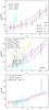 |
Fig. 3 Fraction of blue galaxies as computed in different colours, based on the DS definition from Fig. 1 and colour–colour selection from Fig. 2. It is compared with observational data and with the original Butcher-Oemler curve in B − V, extrapolated to high z as fbl = (z/ 2) − 0.015 (mid panel, dot-long-dashed line). The lower limit for selecting samples is given in terms of redshift-variable absolute MB,MV and MK magnitudes (see text for details). The Poissonian error on fbl is given by σ2(fbl) = Nbl(N − Nbl) /N3 (see De Propris et al. 2004) and shown only for SIM cluster cores in the U − B plot as reference (upper panel). |
4.1. Red and blue fractions
Two main methodologies are commonly applied when measuring the BO effect: either relying on optically selected samples down to a rest-frame MV equivalent to the original BO84 work (e.g. Rakos & Schombert 1995; Fairley et al. 2002; Ascaso et al. 2008; Urquhart et al. 2010; Lerchster et al. 2011), or selecting in observed K-band by applying a brightness limit that is fixed with respect to the characteristic K∗ at each redshift (De Propris et al. 2003; Haines et al. 2009). General results from the latter approach converge to yield lower values of the blue fractions, which raises the suspicion that the BO effect may be partially due to biased photometric selection alone. In particular, De Propris et al. (2003) found that IR-selected blue fractions are lower than optical-selected ones, and both with no redshift trend when performing the same limiting procedure; they impute the gap to a population of starbursting dwarfs or faint spirals that lie on the border of the variable magnitude limit and hence are missed when selecting in terms of K∗.
We compared these observational data, although diverse in their selection criteria, with our blue fractions derived according to the DS mean colour in Fig. 3. Comparing the results obtained in the different colours gives then indications that the BO effect, as originally introduced, is more evident in optical-optical colours than in optical-NIR: here the blue fraction evolves flatter, which also agrees with results by De Propris et al. (2003) or Haines et al. (2009). This is expected, since colours bracketing the 4000 Å break, that is, those with a blue optical colour, are much more sensitive to ongoing star formation, meaning that the physical colour spread will be boosted and the fb will hence increase the bluer the colour. Our galaxies in B − V and U − B fall on a trend that is fairly compatible with the original definition of BO84, which is plotted as the curve fbl = (z/ 2) − 0.015, extrapolated to high z. All the observational estimations based on fixed magnitude criteria on datasets at different redshifts instead lie well above this line. We tested that our SAM curves, when applying this latter selection, are also boosted to the same high levels (not shown in the plot): in particular, they would feature the same steep slope at low redshift, followed by a high plateau from z ≳ 1 (data by Rakos & Schombert 1995; Fairley et al. 2002; Gerke et al. 2007; Urquhart et al. 2010), which is in contrast with the gentler yet steadier slope extrapolated from BO84 over the same interval. On the other hand, single cluster detections at high z, such as those by Lerchster et al. (2011) and Fassbender et al. (2014), are much closer to our models. A fair explanation in this regard is that two effects play a combined role, enhanced in the visual selection: first a more straightforward one due to incompleteness on pure magnitudes, producing an increase in fb because fewer faint red galaxies are detected in most cases at high z. Second, an indirect incompleteness effect on colours as well, which causes an increasing fb towards fainter limiting magnitudes because the red parts are more incomplete: in fact, since both of any observed bands have a well-defined magnitude limit, the incompleteness increases when moving upwards towards redder colours in the colour–magnitude-space at a fixed magnitude; this implies that the red galaxy counts are less complete than the blue galaxy counts, resulting again in a systematical increase of the blue fraction.
For the differences with environments we find that, irrespective of the colour, the blue fraction is higher in groups than in cluster cores (with cluster outskirts in between), both in SIM and in SAM: this environmental component of the BO effect was already highlighted in sevaral studies (see e.g. Urquhart et al. 2010).
Finally, we also note that all our SAM curves (and particularly also SIM clusters) lie lower than another SAM by Menci et al. (2008), who adopted similar selection criteria as ours in U − B, although starting with different recipes for modelling both AGN feedback and strangulation processes.
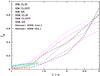 |
Fig. 4 Fraction of star-forming galaxies as a function of redshift, defined according to a threshold of sSFR = 10-10/yr. Data from Haines et al. (2009) at low-z yield fractions computed by defining fixed (orange shaded) or resdshift-variable (cyan shaded) thresholds to star-forming activity estimated from LIR and thoroughly converted to SFR assuming a Kennicutt law. |
In general, colours provide estimates of star formation histories over longer timescales than usual SFR indicators, because they keep memory of past environmental effects; on the other hand, the SFR is a more primary property than colours because it comes as a direct, underived output from models. For the modelled parameter, however, another caveat is that it refers to the actual SFR in the SAM, while in the simulation it is computed as the average over the last Gyr, so that it traces the galaxy cumulative star formation history more than episodic starbursts. Moreover, in observations more reliable estimates of SFR often come from measuring the mid IR re-emission rather than from rest-frame UV/optical data alone (see Saintonge et al. 2008). In Fig. 4 the fraction of star-forming galaxies is plotted, as computed by imposing a threshold of sSFR = 10-10/yr and compared with K-band selected data from Haines et al. (2009) at z ≲ 0.3, who either applied a fixed or redshift-evolving threshold on the LIR-based SFR (shaded orange and cyan regions, respectively). Here, our cluster core curves feature a flatter evolution at z ≲ 0.5 that is consistent with both the observational data sets, followed by a steeper trend: this is more pronounced in the SIM, where they eventually reach values of star-forming galaxies of above 80% at z = 2. For other galaxy classes, the slope begins to steepen at later epochs (z ~ 0.3) onwards.
All in all, the environmental sequence appears to once again be confirmed: inner galaxies are less active than outer and group galaxies. However, the curves from different regions in the SIM tend to converge towards z> 1, hinting at a reversal of the SF-density relation between cluster cores and outskirts at z ≃ 1.5, as recently reported by Santos et al. (2015) at exactly that redshift. In the SAM the three curves instead run almost parallel over time, indicating that the environmental quenching (as measured by the dependence of fbl on the cluster-centric distance) does not change with redshift, as assessed by Raichoor & Andreon (2012b). Finally, the only difference between normal and fossil groups in the SIM (not shown in the figure, where they are unified as average) arises at z ≤ 0.2, when FGs abruptly lose all their star-forming galaxies, while NG galaxies continue their prolongued activity until the present, confirming previous findings of R08.
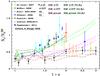 |
Fig. 5 Ratio of luminous-to-faint galaxy numbers in the RS sample, defined from bi-colour separation and by fixed mass thresholds (except the SAM green lines, plotted for reference as to magnitude selection). Error bars are only shown for cluster cores in SIM. The dot-long-dashed curve shows the best fit for z ≤ 1 clusters by Gilbank & Balogh (2008), using fixed thresholds in magnitude equivalent to MV = − 20 and − 18.2. |
4.2. Luminous-to-faint ratio
The LFR (or alternatively the DGR, dwarf-to-giant ratio) is primarily a function of the LF slope, but is also affected by the value of its characteristic luminosity, hence its estimate is degenerate upon variations in both these quantities. In addition, it is also very sensitive to the exact colour cut definition, as discussed in the previous section. The most critical aspect about measuring the LFR is which parts of the LF are considered in the luminous and faint bins. To make the comparison as uniform as possible with observational data, we computed the LFR according to different thresholds, either in luminosity or in mass, with the main purpose of mimicking the completeness limits adopted in most observations. Since using a fixed threshold in magnitude results in an unrealistic increase in the LFR at high z, we chose to separate the two samples either in terms of (fixed) stellar mass, with upper and lower limits given by M∗ = 2 × 10¹⁰ and 4 × 10⁹ M⊙, respectively; or alternatively in terms of magnitude, which must be consistently evolved with redshift to compare galaxies at the same evolutionary stage. In this regard, intervals need to be defined with respect to the evolving characteristic magnitude M∗(z) at a given redshift, which is commonly well approximated with simple stellar population models of formation redshift zf = 3 − 4 (see Andreon et al. 2014). Following De Lucia et al. (2007) for instance, this corresponds to the following interval bins: luminous ≤M∗ + 1.2, M∗ + 1.2< faint ≤M∗ + 3, which in turn translates into the thresholds MV(z = 0) = ( − 20, − 18.2) and MK(z = 0) = ( − 23, − 21.15), by assuming the local characteristic magnitudes from the previous section.
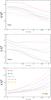 |
Fig. 6 Ratio of stellar masses contained in luminous-to-faint RS galaxies in the SAM for cluster cores (dashed) and averaged cluster outskirts plus groups (dotted), according to the different selection criteria listed. Upper panel: fixed mass limits at M∗ = 2 × 10¹⁰ and 4 × 10⁹ M⊙; middle panel: redshift-variable magnitude limits (see text); bottom panel: fixed magnitude limits at MV = − 20 and − 18.2, or MK = − 23 and − 21. |
All the observational points in Fig. 5 are based on cluster surveys in visual wavebands with apertures of few R500 at z ≤ 1 and mostly display an increasing trend (e.g. Stott et al. 2007; Muñoz et al. 2009; Rudnick et al. 2009). Our results indicate that both SIM and SAM curves are flatter with redshift than most of observations: in fact, they agree best with Andreon’s points (2008, 2014), but also with Fassbender et al. (2014); these are also among the farthest clusters confirmed in the literature, with various degrees of quiescence measured in their cores. Here our RS samples are defined according to the bi-colour separation, but similar results are obtained from the criterion of DS mean colour. For environmental effects on the LFR, no such evidence is firmly established from our results, which therefore cannot confirm previous claims leading to a size or mass segregation, by Bañados et al. (2010) and de Filippis et al. (2011), for example. As another test, the SAM curves obtained by applying a fixed magnitude criterion for selection are plotted alongside in the same figure (green lines): as expected, they instead trail on the steep trend fitted by the SAM in Gilbank & Balogh (2008), valid for clusters up to z ≃ 1. This confirms that the LFR evolution is mostly sensitive to the selection criteria chosen.
The sensitivity of the LFR on the sample selection function is even more evident if the ratio of stellar masses is considered instead of the galaxy numbers, although this cannot be considered as a proper observable; in Fig. 6 SIM are not shown because of their poorer statistics, resulting in larger errors especially at high z, since the mass ratio is strongly affected by even negligible shifts in galaxy numbers. In the mass-selected sample (upper panel) an increasing trend with time is followed by all SAM curves: red galaxies with stellar masses greater than 2 × 10¹⁰ grow their stellar mass by approximately twice especially in cluster cores and for almost all the colour selection criteria, although with different normalizations. Conversely, when the lower limit is set in terms of the same fixed magnitude used in De Lucia et al. (2007) or Gilbank & Balogh (2008), both aiming at reproducing the original procedure by BO84 but with fixed limits, this is reversed and the stellar mass contained in brighter galaxies decreases in time with respect to that in fainter ones (lower panel). The latter behaviour is more consistent with a rapid buildup at the low-mass end of the quiescent stellar mass function, as measured for example by Tomczak et al. (2014) in the field, who found that the total stellar mass density of passive galaxies (complete down to 109 M⊙) has increased since z = 2.5 by a factor of 12, whereas that of star-forming galaxies only by about twice. Finally, an intermediate behaviour between the two previous ones is displayed in the middle panel, where the limits are given in terms of evolving magnitude as aforementioned: in this case the overall trend of the mass ratio is roughly constant over time, especially when measured in K-band, while in V it approximately doubles from z = 2 to present (yellow and blue lines). We tend to favour the latter scenario, as well as the one descending from the mass selection, because it is more physically motivated in its premises.
5. Discussion and conclusions
We have compared observational with theoretical data from two different sources, a cosmological-hydrodynamical simulation and a semi-analytical model. We analyzed proxies of galaxy populations in clusters and groups such as blue fractions and LFR on the RS, extending the analysis over a wide range of optical and NIR wavelength. Both these observables correspond to two major controversial outputs from any galaxy formation model, namely how many red and how many dwarf galaxies are formed with respect to the observed local and high-redshift stellar mass functions. We applied different criteria for defining blue and red galaxies, all redshift-dependent to disentangle the natural colour reddening from the intrinsic evolutionary effects we wished to study. Likewise, we selected our RS samples by defining limits in both MV and MK that are evolving with redshift to take into account the expected luminosity evolution of galaxies, as parametrized by L∗ at each z. The combination of these selection criteria ensures that we account for the naturally bluer rest-frame colours of high-redshift galaxies, given their mean younger age and the higher mean SFR of the overall Universe at that epoch. Our main findings are the following:
-
The blue fraction evolves more markedly when selecting inoptical colours than in K-band. The visual blue fraction(Fig. 3) and the star-forming fraction(Fig. 4) evolve more steeply earlier than z ≃ 0.5,especially in SIM. The much slower evolution at z ≲ 0.5 agrees well withdata by De Propris et al. (2003) orHaines et al. (2009). At high redshift our results areconsistent with spectroscopically confirmed proto-clusters withdeep completeness in galaxy mass, such as Fassbenderet al. (2014) and Andreon et al.(2014).
-
Trends in blue fractions are definitely flatter when they are limited in stellar mass or evolving magnitude instead of by fixed V magnitude (Fig. 3).
-
LFR trends are compatible with the most recent data at high redshift (e.g. Andreon et al. 2014; Fassbender et al. 2014), pointing at very mild evolution, either when selected by mass or by (evolving) magnitude (Fig. 5).
-
The two results of the blue-to-red fractions and LFR are inconsistent with observations that applied fixed thresholds in limiting magnitude or a colour cut upon redshift-spanning surveys, but do instead fairly reproduce their steeper evolution when adopting the same criteria.
-
Testing the different criteria adopted for defining RS galaxies, our conclusion is that choosing a physically motivated redshift-dependent colour threshold is of capital importance. However, of the three sources of uncertainty that we analyzed, the observable results are affected first by the fixed or variable magnitude choice on the lower limit, secondly by the magnitude band itself (visual or K), and thirdly by the colour criterion of those ascertained (see Fig. 6).
-
Normal groups and cluster outskirts present higher blue and star-forming fractions and LFR than cluster cores at any epoch, consistently with a picture where groups are not very efficient at quenching infalling galaxies (see Gerke et al. 2007). In particular for FGs, our results support previous findings by Romeo et al. (2008): the number of blue galaxies only begins to deviate with respect to that of normal groups at z ≲ 0.5 (Fig. 3) because of the much larger portion of red dwarfs in FGs (Fig. 5). This again confirms that star formation history in FGs tends to behave close to cluster cores during the last 4 Gyr of cosmic time, after following the same pattern as normal groups during the previous epoch.
-
A source of discrepancy between SIM and SAM is given at early epoch: cluster cores in SIM display evidence of higher SFR in the past earlier than z ~ 1.5, in agreement with clues from recent detections (e.g. Strazzullo et al. 2013; Santos et al. 2015); in contrast, the redshift dependence of fbl in SAM maintains the same slope among the three galaxy classes and only varies its normalization. This indicates a redshift-independent environmental quenching during the time interval considered. This difference could stem from the epoch of stellar mass assembly, which is generally anticipated in the SAM with respect to SIM (see below).
-
By adopting a mass-selected sample, we also found that the more massive RS galaxies grow their mass at a higher rate than less massive ones (Fig. 6): this reflects that progressively more massive former blue galaxies join the RS after they are quenched (cf. Faber et al. 2007; Cen 2014). We remark that since these are selected as already quiescent galaxies, they are likely to grow in stellar mass through (minor and dry) merger events after entering the RS, thus they contribute to steepen its slope (see De Lucia et al. 2006; Romeo et al. 2008; Guo & White 2008; Jiménez et al. 2011).
We note that in all the plots the differences between SIM and SAM are always much smaller than the typical scatter of the observed data. In general, SAMs produce an excess of stellar mass in early low-mass galaxies that is due to an over-production of stars in low-mass DM haloes, and along with this, they result in a too high fraction of red satellites in clusters (see Fontanot et al. 2009; Guo et al. 2011). Both these manifestations of the same phenomenon are due to galaxies that form very early and evolve almost passively at later times because they follow the hierarchical growth of their DM host haloes too closely: in this respect, a way to overcome this drawback could be decoupling the halo accretion rate from the galaxy SFR (see Weinmann et al. 2012). Various ad hoc models have been proposed to quench early star formation in dwarf galaxies: for example by halting further gas accretion below a certain halo mass threshold (Bouché et al. 2010), or by introducing a two-phase gas split into star-forming and not (Cousin et al. 2015) to reduce the star formation efficiency in low-mass haloes since early epoch. However, in the range of mass below 1010 M⊙, physical processes such as feedback by SNe and stellar winds play a crucial role in galaxy evolution, which still are most likely implemented in a too simplistic way in the models (see Kannan et al. 2014).
In particular, Weinmann et al. (2011) found a red fraction of modelled galaxies too high when compared to Virgo cluster or more generally to less dynamically relaxed clusters such as higher-redshift systems, ascribing it to either an over-efficient quenching of star formation in satellite galaxies (as found by Guo et al. 2011), or to the lack of an efficient stellar stripping or disruption of such galaxies. Nevertheless, the latter channel has been found not to represent a complete solution: Contini et al. (2014), who updated the SAM of De Lucia & Blaizot (2007) with specific prescriptions for stellar stripping, recently addressed the problem of over-predicting low-mass galaxies and demonstrated that it is only partially alleviated thereby, since tidal forces preferentially act on intermediate- to high-mass galaxies. Therefore all present SAMs are facing the same difficulties, given that they normally assume that satellite galaxies are quenched in all haloes, regardless of mass or redshift.
The differences between SIM and SAM mainly arise at z ≥ 1.5, where simulations yield higher SFR (Fig. 4) and lower LFR (Fig. 5). In addition, SAM tends to yield redder colours at any epoch, even when considering only quiescent galaxies and especially in the IR (Fig. 1). In particular, the bulk of star formation in SAM core galaxies occurs fairly earlier than z = 2, whilst these same objects in SIM are still actively forming stars at that epoch. This discrepancy at early epoch can also originate from the more virialized dynamical state of the averaged sample of SAM haloes.
In addition to a difference in resolution effect, chemical enrichment (which is instantaneous in the SAM), diffuse light (which is present as inter-galactic star particles in the SIM, see Sommer-Larsen et al. 2005) and possibly different dwarf modelling, our models also differ in that the simulation does not implement AGN feedback, while the semi-analytical model does: here star formation in the central galaxies is shut off when radio-mode AGN activity is turned on and prevents halo gas from cooling onto the galaxy itself. Therefore SFR in SAM core galaxies can be lower than in SIM, as some massive satellite galaxies are already quenched by AGN feedback before accretion. There is significant evidence today of AGN feedback just at the epoch of interest to the present work, driven by integral-field-observed molecular outflows (see e.g. Brusa et al. 2015; Cresci et al. 2015; Perna et al. 2015). However, from our comparison we see that models including or excluding AGN feedback give similar results for the colour distributions and fractions and the stellar mass function, provided that only galaxy samples excluding the BCGs are considered. On the opposite mass side, our joint results from SIM and SAM converge in not relating any proper dearth of red dwarf galaxies above that epoch, although with the double caveat that detection of red satellites is observationally challenging at z ≳ 1, and that especially SAMs usually meet severe difficulties in reproducing the correct stellar mass function at its faint end.
The emerging picture that we gather is that the main physical mechanisms acting in either of our models, namely cold gas removal by ram pressure stripping on one hand, whose efficiency increases in denser environments, and AGN feedback on the other, which affects the more massive galaxies by virtue of their halo mass, can combine together, and with the aid of a long-lasting sequence of minor and dry merging activity, shape the quenching history of galaxies as a function of both their environment and stellar mass.
Acknowledgments
We thank the referee and also S. Andreon for their useful comments. This work is supported by the 973 program (Nos. 2015CB857000, 2013CB834900), the Foundation for Distinguished Young Scholars of Jiangsu Province (No. BK20140050), the “Strategic Priority Research Program The Emergence of Cosmological Structure” of the CAS (No. XDB09010000) and by China Postdoctoral Science Foundation through grant No. 2015M570488 (AR). A.R. and X.K. are also supported by the NSFC (No. 11333008). E.C. acknowledges the support from the CAS Presidents International Fellowship Initiative (No. 2015PM054). R.F. acknowledges funding from the European Union Seventh Framework Programme (FP7/2007-2013) under grant agreement No. 267251 “Astronomy Fellowships in Italy” (AstroFIt).
References
- Andreon, S. 2008, MNRAS, 386, 1045 [NASA ADS] [CrossRef] [Google Scholar]
- Andreon, S., & Ettori, S. 1999, ApJ, 516, 647 [NASA ADS] [CrossRef] [Google Scholar]
- Andreon, S., Lobo, C., & Iovino, A. 2004, MNRAS, 349, 889 [NASA ADS] [CrossRef] [Google Scholar]
- Andreon, S., Quintana, H., Tajer, M., Galaz, G., & Surdej, J. 2006, MNRAS, 365, 915 [NASA ADS] [CrossRef] [Google Scholar]
- Andreon, S., Newman, A. B., Trinchieri, G., et al. 2014, A&A, 565, A120 [NASA ADS] [CrossRef] [EDP Sciences] [Google Scholar]
- Aragón Salamanca, A., Ellis, R. S., Couch, W. J., & Carter, D. 1993, MNRAS, 262, 764 [NASA ADS] [CrossRef] [Google Scholar]
- Ascaso, B., Moles, M., Aguerri, J. A. L., Sanchez-Janssen, R., & Varela, J. 2008, A&A, 487, 453 [NASA ADS] [CrossRef] [EDP Sciences] [Google Scholar]
- Bañados, E., Hung, Li-W., De Propris, R., & West, M. J. 2010, ApJ, 721, L14 [NASA ADS] [CrossRef] [Google Scholar]
- Bell, E. F., Wolf, C., Meisenheimer, K., et al. 2004, ApJ, 608, 752 [NASA ADS] [CrossRef] [Google Scholar]
- Berrier, J. C., Stewart, K. R., Bullock, J. S., et al. 2009, ApJ, 690, 1292 [NASA ADS] [CrossRef] [Google Scholar]
- Bouché, N., Dekel, A., Genzel, R., et al. 2010, ApJ, 718, 1001 [NASA ADS] [CrossRef] [Google Scholar]
- Brusa, M., Bongiorno, A., Cresci, G., et al. 2015, MNRAS, 446, 2394 [NASA ADS] [CrossRef] [Google Scholar]
- Bruzual, G., & Charlot, S. 2003, MNRAS, 344, 1000 [NASA ADS] [CrossRef] [Google Scholar]
- Bundy, K., Ellis, R. S., & Conselice, C. J. 2005, ApJ, 625, 621 [NASA ADS] [CrossRef] [Google Scholar]
- Butcher, H., & Oemler, A. 1984, ApJ, 285, 426 [NASA ADS] [CrossRef] [Google Scholar]
- Cattaneo, A., Dekel, A., Faber, S. M., & Guiderdoni, B. 2008, MNRAS, 389, 567 [NASA ADS] [CrossRef] [Google Scholar]
- Cen, R. 2014, ApJ, 781, 38 [NASA ADS] [CrossRef] [Google Scholar]
- Chabrier, G. 2003, PASP, 115, 763 [NASA ADS] [CrossRef] [Google Scholar]
- Cirasuolo, M., McLure, R. J., Dunlop, J. S., et al. 2010, MNRAS, 401, 1166 [NASA ADS] [CrossRef] [Google Scholar]
- Contini, E., De Lucia, G., Villalobos, A., & Borgani, S. 2014, MNRAS, 437, 3787 [NASA ADS] [CrossRef] [EDP Sciences] [Google Scholar]
- Couch, W. J., Barger, A. J., Smail, I., Ellis, R. S., & Sharples, R. M. 1998, ApJ, 497, 188 [NASA ADS] [CrossRef] [Google Scholar]
- Cousin, M., Lagache, G., Bethermin, M., Blaizot, J., & Guiderdoni, B. 2015, A&A, 575, A32 [NASA ADS] [CrossRef] [EDP Sciences] [Google Scholar]
- Crawford, S. M., Bershady, M. A., & Hoessel, J. G. 2009, ApJ, 690, 1158 [NASA ADS] [CrossRef] [Google Scholar]
- Cresci, G., Mainieri, V., Brusa, M., et al. 2015, ApJ, 799, 82 [Google Scholar]
- Croton, D. J., Springel, V., White, S. D. M., et al. 2006, MNRAS, 365, 11 [NASA ADS] [CrossRef] [Google Scholar]
- de Filippis, E., Paolillo, M., Longo, G., et al. 2011, MNRAS, 414, 2771 [NASA ADS] [CrossRef] [Google Scholar]
- De Lucia, G., & Blaizot, J. 2007, MNRAS, 375, 2 [NASA ADS] [CrossRef] [Google Scholar]
- De Lucia, G., Springel, V., White, S. D. M., Croton, D., & Kauffmann, G. 2006, 2006, MNRAS, 366, 499 [NASA ADS] [CrossRef] [Google Scholar]
- De Lucia, G., Poggianti, B. M., Aragón-Salamanca, A., et al. 2007, MNRAS, 374, 809 [NASA ADS] [CrossRef] [Google Scholar]
- De Propris, R., Stanford, S. A., Eisenhardt, P. R., & Dickinson, M. 2003, ApJ, 598, 20 [NASA ADS] [CrossRef] [Google Scholar]
- De Propris, R., Colless, M., Peacock, J. A., et al. 2004, MNRAS, 351, 125 [NASA ADS] [CrossRef] [Google Scholar]
- D’Onghia, E., Sommer-Larsen, J., Romeo, A. D., et al. 2005, ApJ, 630, L10 [Google Scholar]
- Diaferio, A., Kauffmann, G., Balogh, M. L., et al. 2001, MNRAS, 323, 999 [NASA ADS] [CrossRef] [Google Scholar]
- Ellingson, E., Lin, H., Yee, H. K. C., & Carlberg, R. G., 2001, ApJ, 547, 609 [NASA ADS] [CrossRef] [Google Scholar]
- Faber, S. M., Willmer, C. N. A., Wolf, C., et al. 2007, ApJ, 665, 265 [NASA ADS] [CrossRef] [Google Scholar]
- Fairley, B. W., Jones, L. R., Wake, D. A., et al. 2002, MNRAS, 330, 755 [NASA ADS] [CrossRef] [Google Scholar]
- Fassbender, R., Nastasi, A., Santos, J. S., et al. 2014, A&A, 568, A5 [NASA ADS] [CrossRef] [EDP Sciences] [Google Scholar]
- Fontanot, F., De Lucia, G., Monaco, P., Somerville, R. S., & Santini, P. 2009, MNRAS, 397, 1776 [NASA ADS] [CrossRef] [Google Scholar]
- Gavazzi, G., Pierini, D., & Boselli, A. 1996, A&A, 312, 397 [NASA ADS] [Google Scholar]
- Gerke, B. F., Newman, J. A., Faber, S. M., et al. 2007, MNRAS, 376, 1425 [NASA ADS] [CrossRef] [Google Scholar]
- Gilbank, D. G., & Balogh, M. L. 2008, MNRAS, 385, L116 [NASA ADS] [CrossRef] [Google Scholar]
- Gilbank, D. G., Yee, H. K. C., Ellingson, E., et al. 2008, ApJ, 673, 742 [NASA ADS] [CrossRef] [Google Scholar]
- Girardi, L., Bertelli, G., Bressan, A., et al. 2002, A&A, 391, 195 [NASA ADS] [CrossRef] [EDP Sciences] [Google Scholar]
- Gladders, D. G., López Cruz, O., Yee, H. K. C., & Kodama, T. 1998, ApJ, 501, 571 [NASA ADS] [CrossRef] [Google Scholar]
- Goto, T., Postman, M., Cross, N. J. G., et al. 2005, ApJ, 621, 188 [NASA ADS] [CrossRef] [Google Scholar]
- Guo, Qi, & White, S. D. M. 2008, MNRAS, 384, 2 [NASA ADS] [CrossRef] [Google Scholar]
- Guo, Qi, White, S., Boylan-Kolchin, M., et al. 2011, MNRAS, 413, 101 [NASA ADS] [CrossRef] [Google Scholar]
- Haines, C. P., Smith, G. P., Egami, E., et al. 2009, ApJ, 704, 126 [NASA ADS] [CrossRef] [Google Scholar]
- Hilton, M., Stanford, S. A., Stott, J. P., et al. 2009, ApJ, 697, 436 [NASA ADS] [CrossRef] [Google Scholar]
- Jiménez, N., Cora, S. A., Bassino, L. P., Tecce, T. E., & Smith Castelli, A. 2011, MNRAS, 417, 785 [NASA ADS] [CrossRef] [Google Scholar]
- Kang, Xi, & van den Bosch, F. C. 2008, ApJ, 676, L101 [NASA ADS] [CrossRef] [Google Scholar]
- Kang, Xi, Jing, Y. P., Mo, H. J., & Borner, G. 2005, ApJ, 631, 21 [NASA ADS] [CrossRef] [Google Scholar]
- Kang, Xi, Jing, Y. P., & Silk, J. 2006, ApJ, 648, 820 [NASA ADS] [CrossRef] [Google Scholar]
- Kang, Xi, van den Bosch, F. C., & Pasquali, A. 2007, MNRAS, 381, 389 [NASA ADS] [CrossRef] [Google Scholar]
- Kang, Xi, Li, M., Lin, W. P., & Elahi, P. J. 2012, MNRAS, 422, 804 [NASA ADS] [CrossRef] [Google Scholar]
- Kannan, R., Stinson, G. S., Macciò, A. V., et al. 2014, MNRAS, 437, 3529 [NASA ADS] [CrossRef] [Google Scholar]
- Kashikawa, N., Takata, T., Ohyama, Y., et al. 2003, ApJ, 125, 53 [Google Scholar]
- Kauffmann, G. 1995, MNRAS, 274, 153 [NASA ADS] [Google Scholar]
- Komatsu, M., Smith, K. M., Dunkley, J., et al. 2011, ApJS, 192, 18 [NASA ADS] [CrossRef] [Google Scholar]
- Krick, J. E., Surace, J. A., Thompson, D., et al. 2008, ApJ, 686, 918 [NASA ADS] [CrossRef] [Google Scholar]
- Lerchster, M., Seitz, S., Brimioulle, F., et al. 2011, MNRAS, 411, 2667 [NASA ADS] [CrossRef] [Google Scholar]
- Lidman, C., Rosati, P., Tanaka, M., et al. 2008, A&A, 489, 981 [NASA ADS] [CrossRef] [EDP Sciences] [Google Scholar]
- Mei, S., Holden, B. P., Blakeslee, J. P., et al. 2009, ApJ, 690, 42 [NASA ADS] [CrossRef] [Google Scholar]
- Menci, N., Rosati, P., Gobat, R., et al. 2008, ApJ, 685, 863 [NASA ADS] [CrossRef] [Google Scholar]
- Muñoz, R. P., Padilla, N. D., & Barrientos, L. F. 2009, MNRAS, 392, 655 [NASA ADS] [CrossRef] [Google Scholar]
- Newman, A. B., Ellis, R. S., Andreon, S., et al. 2014, ApJ, 788, 51 [NASA ADS] [CrossRef] [Google Scholar]
- Peng, Y.-j., Lilly, S. J., Kovač, K., et al. 2010, ApJ, 721, 193 [NASA ADS] [CrossRef] [Google Scholar]
- Perna, M., Brusa, M., Cresci, G., et al. 2015, A&A, 574, A82 [NASA ADS] [CrossRef] [EDP Sciences] [Google Scholar]
- Raichoor, A., & Andreon, S. 2012a, A&A, 537, A88 [NASA ADS] [CrossRef] [EDP Sciences] [Google Scholar]
- Raichoor, A., & Andreon, S. 2012b, A&A, 543, A19 [NASA ADS] [CrossRef] [EDP Sciences] [Google Scholar]
- Romeo, A. D., Portinari, L., & Sommer-Larsen, J. 2005, MNRAS, 361, 983 [NASA ADS] [CrossRef] [Google Scholar]
- Romeo, A. D., Sommer-Larsen, J., Portinari, L., & Antonuccio-Delogu, V. 2006, MNRAS, 371, 548 [NASA ADS] [CrossRef] [Google Scholar]
- Romeo, A. D., Napolitano, N. R., Covone, G., et al. 2008, MNRAS, 389, 13 [NASA ADS] [CrossRef] [Google Scholar]
- Romeo Velonà, A. D., Sommer-Larsen, J., Napolitano, N. R., et al. 2013, ApJ, 770, 155 [NASA ADS] [CrossRef] [Google Scholar]
- Rudnick, G., von der Linden, A., Pelló, R., et al. 2009, ApJ, 700, 1559 [NASA ADS] [CrossRef] [Google Scholar]
- Saintonge, A., Tran, K. H., & Holden, B. P. 2008, ApJ, 685, L113 [NASA ADS] [CrossRef] [Google Scholar]
- Santos, J. S., Altieri, B., Valtchanov, I., et al. 2015, MNRAS, 447, L65 [NASA ADS] [CrossRef] [Google Scholar]
- Schawinski, K., Urry, C. M., Simmons, B. D., et al. 2014, MNRAS, 440, 889 [NASA ADS] [CrossRef] [Google Scholar]
- Sommer-Larsen, J., Romeo, A. D., & Portinari, L. 2005, MNRAS, 357, 478 [NASA ADS] [CrossRef] [Google Scholar]
- Springel, V. 2005, MNRAS, 364, 1105 [NASA ADS] [CrossRef] [Google Scholar]
- Springel, V., White, S. D. M., Tormen, G., & Kauffmann, G. 2001, MNRAS, 328, 726 [Google Scholar]
- Stanford, S. A., Eisenhardt, P. R., & Dickinson, M. 1998, ApJ, 492, 461 [NASA ADS] [CrossRef] [Google Scholar]
- Stott, J. P., Smail, I., Edge, A. C., et al. 2007, ApJ, 661, 95 [NASA ADS] [CrossRef] [Google Scholar]
- Stott, J. P., Pimbblet, K. A., Edge, A. C., Smith, G. P., & Wardlow, J. L. 2009, MNRAS, 394, 2098 [NASA ADS] [CrossRef] [Google Scholar]
- Strazzullo, V., Gobat, R., Daddi, E., et al. 2013, ApJ, 772, 118 [NASA ADS] [CrossRef] [Google Scholar]
- Tomczak, A. R., Quadri, R. F., Tran, K.-Vy H., et al. 2014, ApJ, 783, 85 [NASA ADS] [CrossRef] [Google Scholar]
- Urquhart, S. A., Willis, J. P., Hoekstra, H., & Pierre, M. 2010, MNRAS, 406, 368 [NASA ADS] [CrossRef] [Google Scholar]
- van Dokkum, P. G., Franx, M., Kelson, D. D., et al. 1998, ApJ, 500, 714 [NASA ADS] [CrossRef] [Google Scholar]
- Weinmann, S. M., Lisker, Th., Guo, Qi, Meyer, H. T., & Janz, J. 2011, MNRAS, 416, 1197 [NASA ADS] [CrossRef] [Google Scholar]
- Weinmann, S. M., Pasquali, A., Oppenheimer, B. D., et al. 2012, MNRAS, 426, 2797 [NASA ADS] [CrossRef] [Google Scholar]
- Williams, R. J., Quadri, R. F., Franx, M., van Dokkum, P., & Labbé, I. 2009, ApJ, 691, 1879 [NASA ADS] [CrossRef] [Google Scholar]
- Willmer, C. N. A., Faber, S. M., Koo, D. C., et al. 2006, ApJ, 647, 853 [NASA ADS] [CrossRef] [Google Scholar]
- Zucca, E., Bardelli, S., Bolzonella, M., et al. 2009, A&A, 508, 1217 [NASA ADS] [CrossRef] [EDP Sciences] [Google Scholar]
All Figures
|
Fig. 1 Redshift evolution of the mean rest-frame colours of the DS samples from the SIM: clusters IN (black rhombi), clusters OUT (open circles), normal groups (blue triangles), fossil groups (red squares); and from the SAM (green): clusters IN (dashed lines), clusters OUT (dotted lines), and groups (dot-dashed lines). It is also indicated the difference in colour during the redshift interval: |
| In the text | |
|
Fig. 2 Double-colour diagrams for galaxies more massive than 3 × 10⁹ M⊙, selected by their specific SFR: higher (blue) and lower (red) than 10-11/yr; larger symbols are for SIM, dots for the SAM. Solid lines are given by the fitting formulae that separate the two regions: U − V = 0.5(V − K) − 0.5 for 0 ≤ z< 1, U − V = 0.5(V − K) − 0.6 for 1 ≤ z ≤ 1.5, U − V = 0.45(V − K) − 0.54 for 1.5 <z ≤ 2. |
| In the text | |
|
Fig. 3 Fraction of blue galaxies as computed in different colours, based on the DS definition from Fig. 1 and colour–colour selection from Fig. 2. It is compared with observational data and with the original Butcher-Oemler curve in B − V, extrapolated to high z as fbl = (z/ 2) − 0.015 (mid panel, dot-long-dashed line). The lower limit for selecting samples is given in terms of redshift-variable absolute MB,MV and MK magnitudes (see text for details). The Poissonian error on fbl is given by σ2(fbl) = Nbl(N − Nbl) /N3 (see De Propris et al. 2004) and shown only for SIM cluster cores in the U − B plot as reference (upper panel). |
| In the text | |
|
Fig. 4 Fraction of star-forming galaxies as a function of redshift, defined according to a threshold of sSFR = 10-10/yr. Data from Haines et al. (2009) at low-z yield fractions computed by defining fixed (orange shaded) or resdshift-variable (cyan shaded) thresholds to star-forming activity estimated from LIR and thoroughly converted to SFR assuming a Kennicutt law. |
| In the text | |
|
Fig. 5 Ratio of luminous-to-faint galaxy numbers in the RS sample, defined from bi-colour separation and by fixed mass thresholds (except the SAM green lines, plotted for reference as to magnitude selection). Error bars are only shown for cluster cores in SIM. The dot-long-dashed curve shows the best fit for z ≤ 1 clusters by Gilbank & Balogh (2008), using fixed thresholds in magnitude equivalent to MV = − 20 and − 18.2. |
| In the text | |
|
Fig. 6 Ratio of stellar masses contained in luminous-to-faint RS galaxies in the SAM for cluster cores (dashed) and averaged cluster outskirts plus groups (dotted), according to the different selection criteria listed. Upper panel: fixed mass limits at M∗ = 2 × 10¹⁰ and 4 × 10⁹ M⊙; middle panel: redshift-variable magnitude limits (see text); bottom panel: fixed magnitude limits at MV = − 20 and − 18.2, or MK = − 23 and − 21. |
| In the text | |
Current usage metrics show cumulative count of Article Views (full-text article views including HTML views, PDF and ePub downloads, according to the available data) and Abstracts Views on Vision4Press platform.
Data correspond to usage on the plateform after 2015. The current usage metrics is available 48-96 hours after online publication and is updated daily on week days.
Initial download of the metrics may take a while.