| Issue |
A&A
Volume 581, September 2015
|
|
|---|---|---|
| Article Number | A106 | |
| Number of page(s) | 10 | |
| Section | Stellar structure and evolution | |
| DOI | https://doi.org/10.1051/0004-6361/201526211 | |
| Published online | 16 September 2015 | |
The Araucaria project. Precise physical parameters of the eclipsing binary IO Aquarii
1
Millenium Institute of Astrophysics,
Santiago 22,
Chile
e-mail:
This email address is being protected from spambots. You need JavaScript enabled to view it.
2
Universidad de Concepción, Departamento de
Astronomía, Casilla
160-C, Concepción,
Chile
3
Astrophysics Group, Keele University, Staffordshire, ST5 5BG, UK
4
Warsaw University Observatory, Al. Ujazdowskie 4, 00-478
Warsaw,
Poland
5
Leibniz-Institut für Astrophysik Potsdam,
An der Sternwarte 16,
14482
Potsdam,
Germany
6
Observatoire de Genève, Université de Genève,
51 Ch. des Maillettes,
1290
Sauverny,
Switzerland
7
Department of Physics and Astronomy, Johns Hopkins
University, Baltimore, MD
21218,
USA
8
Department of Physics, University of Warwick,
Coventry
CV4 7AL,
UK
Received: 29 March 2015
Accepted: 18 June 2015
Abstract
Aims. Our aim is to precisely measure the physical parameters of the eclipsing binary IO Aqr and derive a distance to this system by applying a surface brightness – colour relation. Our motivation is to combine these parameters with future precise distance determinations from the Gaia space mission to derive precise surface brightness – colour relations for stars.
Methods. We extensively used photometry from the Super-WASP and ASAS projects and precise radial velocities obtained from HARPS and CORALIE high-resolution spectra. We analysed light curves with the code JKTEBOP and radial velocity curves with the Wilson-Devinney program.
Results. We found that IO Aqr is a hierarchical triple system consisting of a double-lined short-period (P = 2.37 d) spectroscopic binary and a low-luminosity and low-mass companion star orbiting the binary with a period of ≳25 000 d (≳70 yr) on a very eccentric orbit. We derive high-precision (better than 1%) physical parameters of the inner binary, which is composed of two slightly evolved main-sequence stars (F5 V-IV + F6 V-IV) with masses of M1 = 1.569 ± 0.004 and M2 = 1.655 ± 0.004 M⊙ and radii R1 = 2.19 ± 0.02 and R2 = 2.49 ± 0.02 R⊙. The companion is most probably a late K-type dwarf with mass ≈0.6 M⊙. The distance to the system resulting from applying a () surface brightness – colour relation is 255 ± 6 (stat.) ± 6 (sys.) pc, which agrees well with the Hipparcos value of 270+91-55 pc, but is more precise by a factor of eight.
Key words: binaries: eclipsing / binaries: spectroscopic / stars: fundamental parameters / stars: distances / stars: solar-type
© ESO, 2015
1. Introduction
Detached eclipsing binary stars are a very important source of precise stellar parameters, especially of absolute radii and masses. It has been proven that such parameters combined with empirical stellar surface brightness – colour (SBC) relations derived from interferometric measurements (e.g. Kervella et al. 2004; Challouf et al. 2014) result in accurate distance determinations even to extragalactic eclipsing binaries. Indeed, very accurate distances to the two Magellanic Clouds determined with the eclipsing binary method have recently been reported (Pietrzyński et al. 2013; Graczyk et al. 2014). In this method, the SBC relation is used as a tool for predicting the angular diameters of the system components (Lacy 1977). The distance is simply derived by comparing the absolute diameter of a component with its predicted angular diameter. The method involves simple geometric considerations and is therefore a powerful tool for measuring distances with a minimum of modelling assumptions.
However, the procedure may be reversed: using prior knowledge of the distance to a particular detached eclipsing binary, SBC empirical relations can be derived in a way completely independent of interferometry. This basic idea has long been known and was firstly used by Stebbins (1910, 1911) to derive the surface brightness of the two components of Algol and β Aur. Within about 250 pc of the Sun there are ~100 confirmed detached eclipsing binaries with parallaxes measured by the Hipparcos mission (e.g. Kruszewski & Semeniuk 1999; Torres et al. 2010). However, about half of them still lack a detailed analysis of their physical parameters or any analysis at all. These systems comprise components covering a wide range of spectral types from B1 to K0 that is suitable for calibrating precise SBC relations in the corresponding colour ranges. The are several factors that influence the precision of SBC calibrations, most importantly, 1) the uncertainty on absolute dimensions, especially the radii; 2) trigonometric parallax errors; 3) intrinsic variability of the star; and 4) zero-point shifts between different photometric systems.
Recently, a few catalogues of precise absolute dimension determinations from eclipsing binaries have been published (Torres et al. 2010; Eker et al. 2014; Southworth 2014) that cover a wide range of temperatures. However, these catalogues show that for the purpose of SBC calibration, a precise analysis of new eclipsing binaries is needed. For example, Torres et al. (2010, see their Fig. 13) listed 15 components from nine systems (EI Cep, V422 Cyg, RZ Cha, GX Gem, BW Aqr, DM Vir, CD Tau, AI Phe, and V432 Aur) in a region of Teff – log g plane covering a box of 6000–7000 K, 3.6–4.1 dex (F-type subgiants). Despite the number of systems with well-determined masses and radii in this region of parameter space, the calibration of the SBC for these stars is not very reliable because one system lacks a trigonometric parallax (V442 Cyg), three systems have very low quality trigonometric parallaxes (GX Gem, BW Aqr, and DM Vir), the Hipparcos parallax of another system (AI Phe) is inconsistent with the value derived using the eclipsing binary method (Andersen et al. 1988), and one system is magnetically active with distortions to the light curve from star spots (V432 Aur). This leaves only five components in three non-active, detached eclipsing binaries with precise absolute dimension determinations within 250 pc from the Sun, and with secure trigonometric parallaxes.
It is believed that parallax uncertainties from Hipparcos are dominated by statistical errors – photon statistics (e.g. van Leeuwen 2007b). For F-type eclipsing binary with a parallax of 4 mas we expect an error of about 1 mas, or in other words, a relative precision of 25%. To improve this, we could average results from many components over colour bins because the statistical uncertainty would decrease as  , where N is the number of components used in analysis.
The Gaia mission (Perryman et al. 2001) is expected to much improve the Hipparcos distances by minimising statistical uncertainties, and for the F-type system mentioned before, the uncertainty of the parallax should be at most 0.5% (de Bruijne et al. 2015). The SBC calibration would benefit from such precise and accurate Gaia parallaxes obtained for a larger number of detached eclipsing binaries. The photometric distances derived for many of them would also be used as an independent check of Gaia results (if some significant systematic were to occur).
Inhomogeneous photometry causes difficulties with transformations between different photometric systems and zero-point shift uncertainties. The situation somewhat resembles problems occurring with the accurate determination of temperatures and angular diameters using the infrared flux method, where the main error comes from photometric calibration uncertainties (see discussion in Casagrande et al. 2014). Anticipating highly accurate parallaxes from Gaia (precision better than 1%) and the standard precision of present-day radii determination (better then 2%), the systematic error of future SBC calibration would be dominated by photometric and radiative properties of stellar atmosphere uncertainties (Andersen, priv. communication).
Here, we present a detailed analysis of IO Aqr (HD 196991, HIP 102041,  , δ2000 = 00°56′21′′), an eclipsing binary system composed of two mid-F-type stars located in the middle of the Teff – log g plane of the region described above. Despite being relatively bright (V ~ 8.8 mag), this star was not recognised as an eclipsing binary until it was observed with Hipparcos and assigned its variable star name by Kazarovets et al. (1999). Time-series photometry is also available from the Wide-Angle Search for Planets (WASP; Pollacco et al. 2006). During our analysis we discovered that IO Aqr is a triple system, where a close inner binary has a low-mass companion star on a much wider orbit. The system was analysed before by Dimitrov et al. (2004). They derived a set of fundamental parameters for the binary, but did not detect any trace of the tertiary component. Although the companion complicates the interpretation of observations for IO Aqr, the companion is optically faint (less than 1% of the total light in V) and, being on a relatively wide orbit, exerts only long-term perturbations on the inner system, so we have been able to determine precise parameters for both stars in the eclipsing binary component of this hierarchical triple system.
2. Observations
2.1. Photometry
2.1.1. ASAS
The V-band photometry of IO Aqr, publicly available from the ASAS catalogue1 (ACVS; Pojmański 2002), spans from 2001 March 27 to 2009 December 1 and contains 384 good-quality points (flagged “A” in the original data). This photometry was extended by 266 measurements from ASAS-North obtained in a second ASAS station on Haleakala, Hawaii. We also have access to previously unpublished I-band photometry from the ASAS and ASAS-North catalogues that spans from 1998 August 21 to 2009 June 4 and contains 1174 good points. In total we have four ASAS data sets, two in V band and two in I band.
2.1.2. WASP
IO Aqr (1SWASP J204045.47+005621.0) is one of several million bright stars (8 ≲ V ≲ 13) that have been observed by WASP. The WASP survey is described in Pollacco et al. (2006) and Wilson et al. (2008). The survey obtains images of the night sky using two arrays of eight cameras, each equipped with a charge-coupled device (CCD), 200-mm f/1.8 lenses and a broad-band filter (400–700 nm). Two observations of each target field are obtained every 5–10 min using two 30 s exposures. The data from this survey are automatically processed and analysed to identify stars with light curves that contain transit-like features that may indicate the presence of a planetary companion. Light curves are generated using synthetic aperture photometry with an aperture radius of 48 arcsec. The data for all the stars in each target field are processed using the sysrem algorithm (Tamuz et al. 2005) to produce differential magnitudes that are partly corrected for systematic noise trends in the photometry. Data for this study were obtained between 2006 July 4 and 2010 October 6.
2.1.3. HIPPARCOS
We downloaded the Hipparcos photometry in HP magnitudes from a public archive2 . We removed four discrepant high points from the data set and finally had 87 photometric points in total.
2.2. Spectroscopy
2.2.1. HARPS
We obtained spectra of IO Aqr with the High Accuracy Radial velocity Planet Searcher (HARPS; Mayor et al. 2003) on the European Southern Observatory 3.6 m telescope in La Silla, Chile. IO Aqr is a bright target, therefore observations were generally obtained in marginal observing conditions or during twilight. Observations were obtained between 2009 October 10 and 2014 September 10. A total of 17 spectra were secured in high-efficiency (“EGGS”) mode. The exposure times were typically 260 s, resulting in an average signal-to-noise ratio (S/N) per pixel of ~60. All spectra were reduced on-site using the HARPS data reduction software (DRS).
2.2.2. CORALIE
Twenty spectra were obtained with the CORALIE spectrograph on the Swiss 1.2 m Euler telescope at La Silla observatory, Chile, between 2008 October 5 and 2010 November 1. The exposure times varied from 780 s to 1200 s, giving a typical S/N near 5500 Å of 50 per pixel. The spectra were reduced using the automated reduction pipeline.
3. Analysis
3.1. JKTEBOP
We used jktebop3 version 25 (Southworth et al. 2004a,b and references therein) to perform least-squares fits of the ebop light-curve model (Popper & Etzel 1981) to the various photometric data sets.
For the epoch of primary eclipse for each photometric data set, T0, we used the time of mid-eclipse that was closest to the average time of observation for that data set. Other free parameters in the least-squares fit were a normalisation constant, the surface brightness ratio J = S2/S1, where S1 and S2 are the surface brightness of the primary and the secondary star, respectively; the sum of the radii relative to semi-major axis, r1 + r2 = (R1 + R2) /a; the ratio of the radii, k = r2/r1; the orbital inclination, i and the orbital period, Porb. The mass ratio was fixed at the value derived from the spectroscopy described below. We consulted various tabulations of linear limb-darkening coefficients (van Hamme 1993; Díaz-Cordovés et al. 1995; Claret et al. 1995; Claret 2000) and then set the value of xLD for both stars to be equal to a fixed average value from these tabulations. We performed independent least-squares fits to investigate the sensitivity of the other parameters to the assumed value of xLD and accounted for this additional uncertainty when calculating the standard errors on these parameters. We assumed that the orbit is circular and fixed the gravity-darkening coefficients of both stars to 0.2 – this parameter has a negligible effect on the results.
The luminosity ratio and third-light contribution estimated from the analysis of the spectroscopic data were included as constraints in the least-squares fits. The relative weightings of the data were set equal to the root-mean-square (rms) residual of a preliminary fit to each data set. We used the residual permutation method to estimate robust standard errors on the free parameters. The results are given in Table 3, and the fits to the individual light curves are shown in Fig. 1. Further details of these fits are given below.
3.1.1. WASP photometry
We divided the WASP data into eight subsets, each subset comprising the data from one camera and one observing season. Outliers were identified using the residuals from a preliminary light curve model and were removed from the analysis. The number of data points used in the analysis and observation dates of each subset are given in Table 1. We identified between 6 and 25 nights in each subset of data where there was an offset between the data observed on that night and the rest of the data. We modified our version of jktebop to include an offset for the data obtained on each of these nights as additional free parameters in the least-squares fit. The values and standard errors given in Table 3 are the weighted mean and standard error of the mean for the results from these eight least-squares fits. The times of mid-eclipse derived from these least-squares fits are given in Table 2.
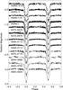 |
Fig. 1 From bottom to top: WASP, ASAS I-band, and ASAS V-band photometry of IO Aqr with jktebop light-curve model fits. The numbers are the ranges of Julian dates for WASP data. |
Log of WASP photometry for IO Aqr.
3.1.2. ASAS photometry
We fitted the four ASAS data sets independently. These data span a wide range of dates of observation with only one observation per night. The effect of the period variations discussed below on the parameters derived is negligible. To derive times of mid-primary eclipse for the period analysis, we divided the data into subsets, each covering approximately 200 nights. We then performed least-squares fits with only T0, J, and a scaling factor as free parameters to derive the times of mid-primary eclipse given in Table 2.
3.1.3. HIPPARCOS photometry
We used Hipparcos photometry to derive the single time of mid-primary eclipse given in Table 2 using the same method as we used for the ASAS data.
Times of mid-primary eclipse for IO Aqr expressed in heliocentric Julian date.
3.2. Period variations
We performed a least-squares fit to data given in Table 2 to derive the following linear ephemeris for the time of mid-primary eclipse in heliocentric Julian date:  The standard error on the final digit of each term is given in parentheses. The residuals from this ephemeris are shown in Fig. 2. It is clear that the period of this binary varies. Assuming that these changes are periodic, we can estimate their minimum period to be >8000 d. This is discussed further in Sect. 3.6.
3.3. Radial velocities
Results of the jktebop fit to the observed LCs.
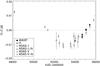 |
Fig. 2 Residuals from the best-fit linear ephemeris to our measured times of mid-primary eclipse. |
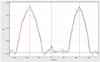 |
Fig. 3 Broadening function power diagram of IO Aqr’s HARPS spectrum taken 2010 September 29 (JD = 2 455 468.5) during full astronomical night with the moon well below horizon. The low-temperature template (Teff = 3950 K) was used to highlight the signal from the third body in the spectrum – the small bump in the middle. The paraboloid curves are rotationally broadened fits to the BF of the primary (right) and the secondary (left), and the continuous vertical lines are the resulting radial velocities of the three stars. |
We used RaVeSpAn (Pilecki et al. 2012) to measure the radial velocities of both stars in the IO Aqr binary system using the broadening function (BF) formalism (Rucinski 1992, 1999). We used templates from the library of synthetic LTE spectra by Coelho et al. (2005). We chose templates to match the estimated effective temperature and gravity of the stars in the binary. The abundance was assumed to be solar. We made preliminary radial velocity fits separately to the HARPS and CORALIE data. There are very small differences in the systemic velocities of both components, but as they are much smaller than dispersion of residuals, we neglected them. The resulting rms of the CORALIE radial velocities is about 30% larger than the rms of HARPS data. The line profiles of both stars are considerably broadened by the rotation of the stars. The projected equatorial rotation velocities of the primary and secondary components are v1sini = 42.6 ± 1.3 km s-1 and v2sini = 52.3 ± 1.1 km -1, respectively. The expected equatorial velocities for assuming synchronous rotation are 46.9 km s-1 and 53.6 km s-1 for the primary and the secondary, respectively, so it appears that rotation rates of both stars are very close to synchronous rotation. The line intensity ratio at 5500 Å is 1.23.
During this analysis, we noticed an additional faint feature in the BF near the radial velocity value 2 km s-1 in one of the spectra – see Fig. 3. We searched for this feature in the other spectra and confirmed its existence in every spectrum. The radial velocity of this feature slightly changes with a spread of about 2 km s-1. We cross-correlated our spectra with different templates and found that the maximum strength of the feature occurs for an assumed template temperature of ~4000 K (assuming solar metallicity). The feature contributes about 1% of the total light at ~6000 Å. Our radial velocity measurements for all three stars are given in Table 4.
RV measurements for IO Aqr.
Observed magnitudes of the system IO Aqr.
The detection of period variations (Sect. 3.2) and third light in the spectra led us to the hypothesis that there is a third body in the system, probably a low-mass main-sequence star. This companion star probably is responsible for the additional signal in the spectrum and the period changes due to the light-time effect, which result from its orbital motion around the main binary.
3.4. Interstellar extinction
The SIMBAD/VizieR database quotes a few different spectral type estimates for IO Aqr: F5 V, F5 III, F6 V, and G0. This range is too broad to be useful for finding intrinsic average colours of the system. Instead, we used extinction maps (Schlegel et al. 1998) with recalibration by Schlafly & Finkbeiner (2011) to determine the reddening in direction of IO Aqr. The total foreground reddening in this direction is E(B − V) = 0.070 ± 0.001 mag. The reddening to IO Aqr is a fraction of this total. To estimate the reddening to IO Aqr, we assumed a simple axisymmetric model of an exponential disc for the distribution of dust within the Milky Way with scale and height lengths taken from Drimmel & Spergel (2001) and assumed a distance to IO Aqr of D = 0.25 kpc (see Sect. 4). For Galactic coordinates of IO Aqr of 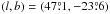 and assuming a solar distance to the Milky Way centre of R0 = 8.3 kpc (Gillessen et al. 2009), we obtain E(B − V)IO Aqr = 0.034 mag. Details of our procedure are given in Suchomska et al. (2015). Maxted et al. (2014) found the scatter of the reddening to individual stars around the value obtained from these reddening maps to be of 0.034 mag.
Additionally, we used a calibration between the equivalent width of the interstellar absorption sodium line NaI D1 and reddening by Munari & Zwitter (1997). We averaged our measurements over several spectra of IO Aqr obtained in orbital quadratures between 2009 and 2014. The interstellar sodium line D1 has one sharp component of constant radial velocity of −10.55 km s-1 The mean equivalent width of this line is 0.082 Å, which results in E(B − V) = 0.019 mag. The scatter of the E(B − V) values for individual stars around the calibration of Munari et al. for low reddening values is approximately 0.04 mag. Both estimates point toward a small extinction in direction of IO Aqr. Finally, we assumed the extinction to be an average of both estimates: E(B − V) = 0.027 ± 0.020 mag.
3.5. Third-light characterisation
We estimated the colour of the third light present in the spectrum using two spectral windows: a blue one ranging from 4000 Å to 5000 Å and a red one ranging from 6000 Å to 6800 Å. These spectral windows approximately correspond to the Johnson B and Johnson-Cousins R photometric bands. Each window was used to calculate the integrated BF profile strength of every component visible in the spectra: W1, W2, W3, where index 1 is for the primary, etc. The profiles were calculated using a template with Teff = 6350 K, log g = 3.00, and solar metallicity. We defined the third light as l3 = W3/ (W1 + W2 + W3). Averaging over several spectra, we obtained l3(B) = 0.0023 and l3(R) = 0.0078. From the observed magnitudes of IO Aqr in the B and R bands, we calculated the magnitudes of the third light in these bands (see Table 5). They correspond to an observed colour (B − R) = 2.11 mag and de-reddened colour (B − R)0 = 2.05. Using Table 5 of Pecaut & Mamajek (2013)4, we found that this colour corresponds to a main-sequence star of spectral type K6 V. Assuming a distance of 255 pc (Sect. 4) and a reddening of E(B − V) = 0.027 (Sect. 3.4) to IO Aqr, we calculated the R absolute magnitude of the companion to be MR = 6.87 mag, which corresponds to a spectral type between K5 V and K6 V. Adding our estimate of the effective temperature given at the end of Sect. 3.3, we conclude that the companion has a spectral type K6 ± 1 subclass. Table 5 gives the magnitude of the companion in different photometric bands assuming colours from Pecaut & Mamajek (2013). The expected contribution of the third light in K band is ~3%.
We found that the derived (B − R) colour depends only slightly on the chosen template, being on average redder for templates with lower effective temperature. Assuming the same distance for IO Aqr and the third-light source, it is unlikely that the source is of spectral type later than M0 V because it would then be too weak to produce a significant BF signal. On the other hand, a star with spectral type earlier than K4 V is also unlikely because it would produce a much stronger BF signal that would match a hotter template (~4600 K).
3.6. Analysis of combined light and radial velocity curves
To perform this analysis we used version 2013 of the Wilson-Devinney program (hereafter WD; Wilson & Devinney 1971; Wilson 1979, 1990; van Hamme & Wilson 2007)5. We cleaned the WASP light curve with 3σ clipping and repeated this cleaning three times. Then we used every third WASP observation to form the final light curve used in the WD analysis. This yielded light curves containing 4730 points in WASP band, 650 points in V band, 1174 points in I band, and 87 points in Hp band.
We set T1 = 6475 K (see Sect. 3.6.1) and [Fe/H] = 0. The grid size was set to N = 40, and standard albedo and gravity brightening for convective stellar atmospheres were chosen. The stellar atmosphere option was used, radial velocity tidal corrections were automatically applied, and no flux-level-dependent weighting was used. We assumed a circular orbit and synchronous rotation for the two components. Logarithmic limb-darkening law were used (Klinglesmith & Sobieski 1970). The starting point for the parameters of the binary system were based on the solutions from the JKTEBOP analysis augmented by dynamical parameters from the preliminary solution obtained with RaVeSpAn, but we also accounted for the influence of the third body on the orbit, as we describe below.
3.6.1. Effective temperature estimates
To estimate the effective temperatures of the eclipsing components, we used a number of (V − K) and (V − I) colour – temperature calibrations (Ramírez & Meléndez 2005; González Hernández & Bonifacio 2009; di Benedetto 1998; Casagrande et al. 2010; Masana et al. 2006; Houdashelt et al. 2000). The intrinsic colours of the two components were calculated from observed magnitudes, estimated reddening, flux ratios derived from the WD model, and from the third-light contribution. As a source for K-band photometry in 2MASS (Cutri et al. 2003) (see Table 5), we used appropriate colour transformations for each calibration. Because flux ratios from the WD model depend on the input temperatures, we iterated the estimation of temperatures a few times. The resulting temperatures are averages from all used calibrations. For the primary and secondary they are 6475 ± 85 K and 6331 ± 69 K, respectively, with errors calculated as the standard deviation. When the reddening and zero-point uncertainties of the photometry are added, the total errors of the temperature determination are 138 K and 125 K for the primary and the secondary, respectively.
3.6.2. Analysis including the third body
We assumed that the changes in orbital period are caused entirely by the light-time effect (Woltjer 1922; Irwin 1959; van Hamme & Wilson 2007). Changes in the orbital period of the inner binary due to gravitational interaction between the three bodies are expected to be at least two orders of magnitude smaller than the variation seen in Fig. 2 (Rappaport et al. 2013, their Eq. (10)). A preliminary analysis of our radial velocities showed that the systemic velocity is γ ≈ 10 km s-1. Dimitrov et al. (2004) reported a much lower systemic velocity of −2 km s-1 from their observations taken in Rozen Observatory with the 2.0 m RCC telescope, which is equipped with a Coudé spectrograph. Their spectra were taken in 2001, so there is a difference of about nine years to our spectra. We initially interpreted the change of the systemic velocity as a sign of interaction between the binary and the third body. However, we quickly realized that the magnitude of the systemic velocity change (~12 km s-1) is much too large: if this were real, we would expect much larger O−C residuals from the linear ephemeris given in Sect. 3.2. We concluded that there is a large systematic zero-point offset in velocities derived from our spectra and the Rozen spectra, and because their radial velocities are on average of lower accuracy than ours, we dropped them from our analysis.
In the analysis we adjusted the following parameters describing the inner binary of IO Aqr: the binary orbital period P, the zero-epoch of the primary minimum HJD0, the systemic velocity γ, the temperature of the secondary T2, the orbital inclination i, the two surface potentials Ω1 and Ω2, the semi-major axis a, the mass ratio q, and the primary star luminosity L1 in each photometric band.
The O−C diagram shows that our eclipse timing and radial velocity data probably cover only a small fraction of the orbital period of the third body, P3. In this case, the third body orbital parameters are not uniquely determined. A striking feature of our radial velocities is the lack of significant changes in the systemic velocity of the inner binary or the mean radial velocity of the third body. Moreover, the shape of the O−C diagram suggests a highly eccentric and long-period third-body orbit. It was also clear from our trial solutions that the orbital period P3 and the eccentricity e3 strongly correlate, as is the case for the longitude of periastron ω3 and the time of the upper spectroscopic conjunction T03. For this reason, we decided to find solutions within a grid of possible periods P3. The additional fitted parameters were those describing the third-body orbit: eccentricity e3, longitude of the periastron ω3, semi-major axis a3, and the moment of the upper spectroscopic conjunction T03. We also assumed that the outer orbit is seen edge-on (i3 = 90 deg).
We decided to divide the third-body parameters into three groups – {e3, T03}, {ω3}, and {a3, T03}. We iteratively fitted these three parameter groups with the parameters of the inner binary (P, HJD0, γ, T2, i, Ω1, Ω2, a, q, and L1) until we achieved no improvement in χ2 for a given value of P3. We repeated this procedure for many orbital periods P3 within a range of from 8000 to 50 000 days. We could not find any acceptable third-body solutions for periods shorter than about 25 000 days. The reason is that the radial velocity difference between the inner binary systemic velocity and the radial velocity of the third body (ΔVr ≈ 8 km s-1) causes a tension with the shape of the O−C curve. The tension is only relaxed for P3> 25 000 days. Periods longer than 50 000 d require a very high eccentricity of the outer orbit (e3> 0.85). In all cases the inferred minimum mass of the third body is about 0.6 M⊙. The specific solution for P3 = 30 000 days is reported in Table 6. Figure 4 presents the fit to the radial velocity data given in Table 4 assuming a constant orbital period during the time span of our spectroscopic data.
Results of the final WD analysis including the third body.
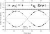 |
Fig. 4 Radial velocity solution of IO Aqr. The lower panel shows the model predictions with continous lines from the WD code calculated for a constant orbital period of P = 2.368137 d. Overplotted are radial velocities for the primary (denoted 1) and the secondary (denoted 2). The dotted line corresponds to the systemic velocity of 9.66 km s-1 corresponding to a mean epoch of CORALIE and HARPS spectra. The upper panel shows residuals from the model fit. |
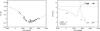 |
Fig. 5 Left panel: O−C residuals of the observed times of primary minimum of IO Aqr assuming the linear ephemeris from Table 6 and predicted O−C caused by the light-time effect from our third-body solution – continous line. Right panel: predicted radial velocity changes of the binary mass centre (continuous line denoted 1+2) and the third body (dashed line denoted 3). The horizontal line corresponds to the heliocentric frame systemic velocity of the whole triple system. The individual binary mass centre velocities from HARPS are marked by filled circles and CORALIE velocities by open circles. The velocities of the third body were binned into seasonal means. |
Figure 5 presents the fit to the O−C residuals of observed minima times from Table 2 and the expected radial velocity changes of the inner binary mass centre of IO Aqr and the third body. To calculate the binary centre-of-mass velocities V1 + 2, we used radial velocities from Table 4 and the equation  (1)where V1,2 denotes radial velocities for the primary and the secondary, respectively, and q is the mass ratio. The asymmetric minimum in the O−C diagram coincides with the periastron passage of the third body near JD 2 452 600. The O−C diagram shows that our final solution for the third body orbit does not fit the Hipparcos data. Forcing a good fit for this one outlier results in stronger binary centre-of-mass radial velocity changes and produces significant residua in the radial velocities. A possible explanation is that we underestimated the error on Hipparcos minimum timing. It is also clear that we only cover a relatively small part of the whole third-body orbit, and much room for improvement probably still exists.
Physical parameters of IO Aqr components.
3.7. Physical parameters
The physical parameters of the components of IO Aqr are presented in Table 7. Our spectral type estimate is based on the derived effective temperatures and the calibration by Pecaut & Mamajek (2013); it is consistent with the spectral classification given by Houk & Swift (1999). The mean radii given are the radius of a sphere with the same volume as the star. The distortions from a perfect sphere defined as (rpoint − rpole) /rmean are 2.3% and 3.2% for the primary and the secondary star, respectively. Errors on luminosities were calculated from uncertainties of the distance estimate and the reddening and bolometric corrections used. The bolometric corrections reported in Table 7 were taken from Casagrande et al. (2010). The fractional precision of derived masses is 0.25% and 0.24% for the primary and the secondary, respectively.
Dimitrov et al. (2004) reported two possible solutions for absolute parameters of IO Aqr denoted as A and B. It becomes evident that our solution lies somewhere between these solutions. However, we were able to significantly refine the parameters of the system. The radii of the two stars are too large for their mass or for their temperature if we were to assume that they are main-sequence stars, as was also pointed out by Dimitrov et al. (2004). We compared our results with stellar isochrones from the Padova and Trieste Stellar Evolutionary Code (PARSEC; Bressan et al. 2012)6. We fitted masses, luminosities, and temperatures of the components. As we have no confident metallicity estimate for this star (the SIMBAD database quotes some estimates made under the assumption that IO Aqr is a single star), we also fitted this parameter. The position of the stars in the Hertzsprung-Russell (H-R) diagram and their measured masses are only matched using isochrones for metallicities [ M / H ] ≈ + 0.3 – see Fig. 6. The estimated age of the system is 1.88 ± 0.10 Gyr. We confirm the finding of Dimitrov et al. (2004) that the two stars are still before the turn-off point in their evolution.
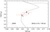 |
Fig. 6 H-R diagram with the primary (1) and the secondary (2) components of IO Aqr marked. Overplotted is the PARSEC isochrone that provides the best match to M, L, and Teff of the two stars, corresponding to an age of 1.88 Gyr. Dots on the isochrone correspond to the position of the best fit. The zero-age main-sequence (ZAMS) is also shown. |
Our absolute parameters do not depend on the orbital solution for the third body. The third body only affects the timing of the eclipses and, to a lesser extent, the estimates of the distance and effective temperatures. Our solutions without the third body (Sect. 3.1.1) yield model parameters that are consistent with those reported in Table 6. The high precision of the derived physical parameters makes IO Aqr another eclipsing binary star on a list of systems that have a precision of the absolute dimension determination better than 3% (e.g. Torres et al. 2010).
4. Distance and space velocity
The distance to the system was derived using two calibrations of visual surface brightness versus (V − K) colour relations (Kervella et al. 2004; di Benedetto 2005) based on measurements of the interferometric stellar angular diameters. The 2MASS K-band magnitude was tranformed onto the Johnson photometric system using transformation equations from Bessell & Brett (1988) and Carpenter (2001)7. The magnitudes were de-reddened with E(B − V) = 0.027 mag. To derive individual K-band magnitudes of the components, we used the K-band light ratio extrapolated from the WD model l21(K) = 1.262 and the third-light contribution l3(K) = 0.030. The resulting de-reddened Johnson V-band and K-band magnitudes for the two stars are V1 = 9.601 mag, V2 = 9.422 mag, and K1 = 8.505 mag, K2 = 8.252 mag. The distance to IO Aqr derived from the SBC relations reported by Kervella et al. (2004) and di Benedetto (2005) are 257.2 pc and 252.2 pc, respectively. The resulting average distance is 255 pc, corresponding to a distance modulus m − M = 7.030 mag.
The systematic errors contribute as follows: the uncertainty of the empirical calibrations of the surface brightness (0.040 mag error in distance modulus), the uncertainty of the extinction law (0.005 mag), the metallicity dependence of the surface brightness relations (0.004 mag), and the zero-point errors of V- and K-band photometry (0.030 mag in total). When we combine the contributions in quadrature, we have a total systematic error of 0.051 mag. The total statistical error comes from the uncertainty in the semi-major axis (0.005 mag), the uncertainty of the sum of fractional radii r1 + r2 (0.010 mag), the uncertainty of the third light (0.022 mag), the errors of V- and K-band magnitudes (0.007 and 0.033 mag, respectively), the reddening uncertainty (0.015 mag), the error of the mean of the two calibrations (0.021 mag), and from separating the magnitudes (0.002 mag). When we combine these uncertainties in quadrature, we have a total statistical error of 0.049 mag. When the errors in distance modulus are translated into errors in parsecs, the final result is 255 ± 6 (stat.) ± 6 (syst.) pc. The distance corresponds to a parallax of 3.93 ± 0.13 mas (total error).
The important consistency check of model parameters we derived (especially their radii and luminosity ratio in different bands) is the distance to each of the system components returned by our procedure. In our case, the distance moduli of the two stars agree excellently well: they are different by less than 0.001 mag for each of the surface brightness calibration used.
The parallax to the binary was determined by the Hipparcos satellite mission. The first published full data reduction (Perryman et al. 1997) gave 5.42 ± 1.46 mas. Subsequently, a new data reduction (van Leeuwen 2007a,b) reported a distinctly smaller parallax of 3.71 ± 0.94 mas. Dimitrov et al. (2004) used an eclipsing binary bolometric flux scaling method and derived a distance to IO Aqr of 256 pc, corresponding to a parallax of 3.91 mas. However, they neither included any third light in their considerations nor gave a distance error estimate. Both of the latter distance determinations agree very well within the uncertainties with our derived distance.
The proper motion of IO Aqr given by van Leeuwen (2007b) is (μαcosδ,μδ) = (−4.59 ± 1.00, −22.42 ± 0.84) mas yr-1. That proper motion expressed in Galactic coordinates is (μlcosb,μb) = (−21.7 ± 1.2, −7.4 ± 0.4) mas yr-1 using the transformations given by Poleski (2013). The transverse velocity in Galactic coordinates is (−26.2 ± 1.5, −8.9 ± 0.5) km s-1. Heliocentric Galactic space velocity components, that is, not corrected for solar peculiar motion, were calculated using the equations given by Johnson & Soderblom (1987), and we obtained (u,v,w) = (21.8 ± 0.6, −14.9 ± 1.6, −11.5 ± 0.8) km s-1. The values and uncertainties given do not take into account possible systematic errors caused by a long-term proper motion drift of the inner binary induced by the third body. At the moment, we have insufficient information to correct for this effect.
5. Final remarks
With the high-precision data now available, we have been able to show that IO Aqr is a hierarchical triple star system with a low-luminosity and low-mass companion on a wide eccentric orbit. For the purpose of accurate SBC calibration, pure eclipsing binaries (i.e. without stellar companions) are preferred. However, when the physical properties, especially the luminosity, of a tertiary companion are well determined or/and the flux of the companion in optical and NIR is negligible, a given eclipsing binary can be used safely. A criterion is the degree of calibration precision we wish to obtain: 1% of precision demands that the tertiary contribution in V and K bands should be at most comparable with this limit. The companion of IO Aqr is faint enough in the optical to be ignored, and its estimated K-band contribution is still small, so that it has a negligible effect on the calculated angular diameters of the IO Aqr components. Using the SBC calibration of di Benedetto (2005), the predicted angular diameters are 0.081 ± 0.002 mas and 0.092 ± 0.002 mas for the primary and the secondary, respectively.
We derived high-precision absolute dimensions of IO Aqr that are among the most precise parameters of F-type stars published to date. Nonetheless, our temperature determination (precision 2%) can be improved by using dedicated Strömgren photometry or by a detailed atmospheric analysis of the separated spectra. We leave this to future work on IO Aqr.
Acknowledgments
We extensively used the SIMBAD/Vizier database in our research. We also used the uncertainties python package. We would like to thank the referee D. Pourbaix for his constructive comments on the paper and the staff of the ESO La Silla observatory for their support during the observations. We also thank W. van Hamme for his valuable comments about modelling of a third body with the Wilson-Devinney code. We (D.G., W.G., G.P.) gratefully acknowledge financial support for this work from the BASAL Centro de Astrofisica y Tecnologias Afines (CATA) PFB-06/2007, and from the Millenium Institute of Astrophysics (MAS) of the Iniciativa Cientifica Milenio del Ministerio de Economia, Fomento y Turismo de Chile, project IC120009. A.G. acknowledges support from FONDECYT grant 3130361. We (D.G., B.P., G.P., P.K., K.S.) gratefully acknowledge financial support for this work from the Polish National Science Center grant MAESTRO 2012/06/A/ST9/00269, the TEAM subsidy from the Foundation for Polish Science (FNP) and NCN grant DEC-2011/03/B/ST9/02573. R.I.A. acknowledges funding from the Swiss National Science Foundation.
References
- Andersen, J., Clausen, J. V., Gustafsson, B., et al. 1988, A&A, 196, 128 [NASA ADS] [Google Scholar]
- Bessell, M. S., & Brett, J. M. 1988, PASP, 100, 1134 [NASA ADS] [CrossRef] [Google Scholar]
- Bressan, A., Marigo, P., Girardi, L., et al. 2012, MNRAS, 427, 127 [NASA ADS] [CrossRef] [Google Scholar]
- Carpenter, J. M. 2001, AJ, 121, 2851 [NASA ADS] [CrossRef] [Google Scholar]
- Casagrande, L., Ramirez, I., Meléndez, J., Bessell, M., & Asplund, M. 2010, A&A, 512, A54 [NASA ADS] [CrossRef] [EDP Sciences] [Google Scholar]
- Casagrande, L., Portinari, L., Glass, I. S., et al. 2014, MNRAS, 439, 2060 [Google Scholar]
- Challouf, M., Nardetto, N., Mourard, D., et al. 2014, A&A, 570, A104 [NASA ADS] [CrossRef] [EDP Sciences] [Google Scholar]
- Claret, A. 2000, A&A, 363, 1081 [NASA ADS] [Google Scholar]
- Claret, A., Diaz-Cordoves, J., & Gimenez, A. 1995, A&AS, 114, 247 [NASA ADS] [Google Scholar]
- Coelho, P., Barbuy, B., Meléndez, J., Schiavon, R. P., & Castilho, B. V. 2005, A&A, 443, 735 [NASA ADS] [CrossRef] [EDP Sciences] [Google Scholar]
- Cutri, R. M., Skrutskie, M. F., van Dyk, S., et al. 2003, VizieR, Online Data Catalogue: II/246 [Google Scholar]
- de Bruijne, J. H. J., Rygl, K. L. J., & Antoja, T. 2015, ArXiv e-prints [arXiv:1502.00791] [Google Scholar]
- Diaz-Cordoves, J., Claret, A., & Gimenez, A. 1995, A&AS, 110, 329 [NASA ADS] [Google Scholar]
- di Benedetto, G. P. 1998, A&A, 339, 858 [NASA ADS] [Google Scholar]
- di Benedetto, G. P. 2005, MNRAS, 357, 174 [NASA ADS] [CrossRef] [Google Scholar]
- Dimitrov, W., Kolev, D., & Schwarzenberg-Czerny, A. 2004, A&A, 417, 689 [NASA ADS] [CrossRef] [EDP Sciences] [Google Scholar]
- Drimmel, R., & Spergel, D. N. 2001, ApJ, 556, 181 [NASA ADS] [CrossRef] [Google Scholar]
- Eker, Z., Bilit, S., Soydugan, F., et al. 2014, PASA, 31, 24 [CrossRef] [Google Scholar]
- Gillessen, S., Eisenhauer, F., Fritz, T. K., et al. 2009, ApJ, 707, L114 [NASA ADS] [CrossRef] [Google Scholar]
- González Hernández, J. I., & Bonifacio, P. 2009, A&A, 497, 497 [NASA ADS] [CrossRef] [EDP Sciences] [Google Scholar]
- Graczyk, D., Pietrzyński, G., Thompson, I. B., et al. 2014, ApJ, 780, 59 [NASA ADS] [CrossRef] [Google Scholar]
- Høg, E., Fabricius, C., Makarov, V. V., et al. 2000, A&A, 357, 367 [NASA ADS] [Google Scholar]
- Houdashelt, M. L., Bell, R. A., & Sweigert, A V., 2000, AJ, 119, 1448 [Google Scholar]
- Houk, N., & Swift, C., 1999, Michigan Catalogue of Two-dimensional Spectral Types for the HD Stars Vol. 5. Declinations −12 deg to +05 deg. Department of Astronomy, University of Michigan, Ann Arbor, MI, USA [Google Scholar]
- Irwin, J. B. 1959, AJ, 64, 149 [NASA ADS] [CrossRef] [Google Scholar]
- Johnson, D. R. H., & Soderblom, D. R. 1987, AJ, 93, 864 [NASA ADS] [CrossRef] [Google Scholar]
- Kazarovets, A. V., Samus, N. N., Durlevich, O. V., et al. 1999, IBVS, No. 4659 [Google Scholar]
- Kervella, P., Thévenin, F., Di Folco, E., & Ségransan, D. 2004, A&A, 426, 297 [NASA ADS] [CrossRef] [EDP Sciences] [Google Scholar]
- Kruszewski, A., & Semeniuk, I. 1999, Acta Astron., 49, 561 [NASA ADS] [Google Scholar]
- Lacy, C. H. 1977, ApJ, 213, 458 [NASA ADS] [CrossRef] [Google Scholar]
- Masana, E., Jordi, C., & Ribas, I. 2006, A&A, 450, 735 [NASA ADS] [CrossRef] [EDP Sciences] [Google Scholar]
- Maxted, P. F. L., Bloemen, S., Heber, U., et al. 2014, MNRAS, 437, 1681 [NASA ADS] [CrossRef] [Google Scholar]
- Mayor, M., Pepe, F., Queloz, D., et al. 2003, The Messenger, 114, 20 [NASA ADS] [Google Scholar]
- Munari, U., & Zwitter, T. 1997, A&A, 318, 269 [NASA ADS] [Google Scholar]
- Pecaut, M. J., & Mamajek, E. E. 2013, ApJS, 208, 9 [NASA ADS] [CrossRef] [Google Scholar]
- Perryman, M. A. C., Lindegren, L., Kovalevsky, J., et al. 1997, A&A, 323, L49 [NASA ADS] [Google Scholar]
- Perryman, M. A. C., de Boer, K. S., Gilmore, G., et al. 2001, A&A, 369, 339 [NASA ADS] [CrossRef] [EDP Sciences] [Google Scholar]
- Pickles, A., & Depagne, E. 2010, PASP, 122, 1437 [NASA ADS] [CrossRef] [Google Scholar]
- Pietrzyński, G., Graczyk, D., Gieren, W., et al. 2013, Nature, 495, 76 [NASA ADS] [CrossRef] [PubMed] [Google Scholar]
- Pilecki, B., Konorski, P., & Górski, M. 2012, From Interacting Binaries to Exoplanets, IAU Symp., 282, 301 [NASA ADS] [Google Scholar]
- Pojmański, G., 2002, Acta Astron., 52, 397 [Google Scholar]
- Poleski, R. 2013, ArXiv e-prints [arXiv:1306.2945] [Google Scholar]
- Pollacco, D. L., Skillen, I., Collier Cameron, A., et al. 2006, PASP, 118, 1407 [NASA ADS] [CrossRef] [Google Scholar]
- Popper, D. M., & Etzel, P. B. 1981, AJ, 86, 102 [NASA ADS] [CrossRef] [Google Scholar]
- Ramírez, I., & Meléndez, J. 2005, ApJ, 626, 465 [NASA ADS] [CrossRef] [Google Scholar]
- Rappaport, S., Deck, K., Levine, A., et al. 2013, ApJ, 768, 33 [NASA ADS] [CrossRef] [Google Scholar]
- Rucinski, S. M. 1992, AJ, 104, 1968 [NASA ADS] [CrossRef] [Google Scholar]
- Rucinski, S. M. 1999, in Precise Stellar Radial Velocities, eds. J. B. Hearnshaw, & C. D. Scarfe, IAU Colloq. 170, ASP Conf. Ser., 185, 82 [Google Scholar]
- Schlafly, E. F., & Finkbeiner, D. P. 2011, ApJ, 737, 103 [NASA ADS] [CrossRef] [Google Scholar]
- Schlegel, D. J., Finkbeiner, D. P., & Davis, M. 1998, ApJ, 500, 525 [NASA ADS] [CrossRef] [Google Scholar]
- Southworth, J. 2014, ArXiv e-prints [arXiv:1411.5517] [Google Scholar]
- Southworth, J., Maxted, P. F. L., & Smalley, B. 2004a, MNRAS, 351, 1277 [NASA ADS] [CrossRef] [Google Scholar]
- Southworth, J., Zucker, S., Maxted, P. F. L., & Smalley, B. 2004b, MNRAS, 355, 986 [NASA ADS] [CrossRef] [Google Scholar]
- Stebbins, J. 1910, ApJ, 32, 185 [NASA ADS] [CrossRef] [Google Scholar]
- Stebbins, J. 1911, ApJ, 34, 112 [NASA ADS] [CrossRef] [Google Scholar]
- Suchomska, K., Graczyk, D., Smolec, R., et al. 2015, MNRAS, 451, 5170 [Google Scholar]
- Tamuz, O., Mazeh, T., & Zucker, S. 2005, MNRAS, 356, 1466 [NASA ADS] [CrossRef] [Google Scholar]
- Torres, G., Andersen, J., & Giménez, A. 2010, A&AR, 18, 67 [Google Scholar]
- van Hamme, W. 1993, AJ, 106, 2096 [NASA ADS] [CrossRef] [Google Scholar]
- van Hamme, W., & Wilson, R. E. 2007, ApJ, 661, 1129 [Google Scholar]
- van Leeuwen, F. 2007a, Hipparcos, the new reduction of the raw data (Dordrecht: Springer) [Google Scholar]
- van Leeuwen, F. 2007b, A&A, 474, 653 [NASA ADS] [CrossRef] [EDP Sciences] [Google Scholar]
- Wilson, R. E. 1979, ApJ, 234, 1054 [NASA ADS] [CrossRef] [Google Scholar]
- Wilson, R. E. 1990, ApJ, 356, 613 [NASA ADS] [CrossRef] [Google Scholar]
- Wilson, R. E., & Devinney, E. J. 1971, ApJ, 166, 605 [NASA ADS] [CrossRef] [Google Scholar]
- Wilson, D. M.,Gillon, M., Hellier, C., et al. 2008, ApJ, 675, L113 [NASA ADS] [CrossRef] [Google Scholar]
- Woltjer, J. 1922, B.A.N., 1, 93 [Google Scholar]
- Zacharias, N., Monet, D. G., Levine, S. E., et al. 2004, BAAS, 36, 1418 [Google Scholar]
All Tables
All Figures
|
Fig. 1 From bottom to top: WASP, ASAS I-band, and ASAS V-band photometry of IO Aqr with jktebop light-curve model fits. The numbers are the ranges of Julian dates for WASP data. |
| In the text | |
|
Fig. 2 Residuals from the best-fit linear ephemeris to our measured times of mid-primary eclipse. |
| In the text | |
|
Fig. 3 Broadening function power diagram of IO Aqr’s HARPS spectrum taken 2010 September 29 (JD = 2 455 468.5) during full astronomical night with the moon well below horizon. The low-temperature template (Teff = 3950 K) was used to highlight the signal from the third body in the spectrum – the small bump in the middle. The paraboloid curves are rotationally broadened fits to the BF of the primary (right) and the secondary (left), and the continuous vertical lines are the resulting radial velocities of the three stars. |
| In the text | |
|
Fig. 4 Radial velocity solution of IO Aqr. The lower panel shows the model predictions with continous lines from the WD code calculated for a constant orbital period of P = 2.368137 d. Overplotted are radial velocities for the primary (denoted 1) and the secondary (denoted 2). The dotted line corresponds to the systemic velocity of 9.66 km s-1 corresponding to a mean epoch of CORALIE and HARPS spectra. The upper panel shows residuals from the model fit. |
| In the text | |
|
Fig. 5 Left panel: O−C residuals of the observed times of primary minimum of IO Aqr assuming the linear ephemeris from Table 6 and predicted O−C caused by the light-time effect from our third-body solution – continous line. Right panel: predicted radial velocity changes of the binary mass centre (continuous line denoted 1+2) and the third body (dashed line denoted 3). The horizontal line corresponds to the heliocentric frame systemic velocity of the whole triple system. The individual binary mass centre velocities from HARPS are marked by filled circles and CORALIE velocities by open circles. The velocities of the third body were binned into seasonal means. |
| In the text | |
|
Fig. 6 H-R diagram with the primary (1) and the secondary (2) components of IO Aqr marked. Overplotted is the PARSEC isochrone that provides the best match to M, L, and Teff of the two stars, corresponding to an age of 1.88 Gyr. Dots on the isochrone correspond to the position of the best fit. The zero-age main-sequence (ZAMS) is also shown. |
| In the text | |
Current usage metrics show cumulative count of Article Views (full-text article views including HTML views, PDF and ePub downloads, according to the available data) and Abstracts Views on Vision4Press platform.
Data correspond to usage on the plateform after 2015. The current usage metrics is available 48-96 hours after online publication and is updated daily on week days.
Initial download of the metrics may take a while.