| Issue |
A&A
Volume 581, September 2015
|
|
|---|---|---|
| Article Number | L7 | |
| Number of page(s) | 6 | |
| Section | Letters | |
| DOI | https://doi.org/10.1051/0004-6361/201525918 | |
| Published online | 22 September 2015 | |
A HARPS view on K2-3⋆,⋆⋆
1
Univ. Grenoble Alpes, IPAG,
38000
Grenoble,
France
e-mail:
This email address is being protected from spambots. You need JavaScript enabled to view it.
2
CNRS, IPAG, 38000
Grenoble,
France
3
Instituto de Astrofísica e Ciências do Espaço, Universidade do
Porto, CAUP, Rua das
Estrelas, 4150-762
Porto,
Portugal
4
Stellar Astrophysics Centre, Department of Physics and Astronomy,
Aarhus University, Ny Munkegade
120, 8000
Aarhus C,
Denmark
5
Aix-Marseille Université, CNRS, LAM (Laboratoire d’Astrophysique
de Marseille) UMR 7326, 13388
Marseille,
France
6
Observatoire Astronomique de l’Université de Genève,
51 chemin des Maillettes,
1290
Versoix,
Switzerland
7
Observatoire de Haute Provence, 04670 Saint-Michel l’Observatoire,
France
8
Institut d’Astrophysique de Paris, UMR 7095 CNRS, Université
Pierre & Marie Curie, 98bis boulevard Arago, 75014
Paris,
France
9
Departamento de Física, Universidade Federal do Rio Grande do
Norte, 59072-970
Natal, RN, Brazil
10
Departamento de Astronomía, Universidad de Chile,
1058
Santiago,
Chile
11
Departamento de Física e Astronomia, Faculdade de Ciências,
Universidade do Porto, Rua do Campo
Alegre 687, 4169-007
Porto,
Portugal
Received: 18 February 2015
Accepted: 27 August 2015
Abstract
K2 space observations recently found that three super-Earths transit the nearby M dwarf K2-3. The apparent brightness and the small physical radius of their host star rank these planets amongst the most favourable for follow-up characterisations. The outer planet orbits close to the inner edge of the habitable zone and might become one of the first exoplanets searched for biomarkers using transmission spectroscopy. We used the HARPS velocimeter to measure the mass of the planets. The mass of planet b is 8.4 ± 2.1 M⊕, while our determination of those planets c and d are affected by the stellar activity. With a density of 4.32+2.0-0.76 g cm-3, planet b is probably mostly rocky, but it could contain up to 50% water.
Key words: planetary systems / stars: late-type / techniques: radial velocities / techniques: photometric
Based on observations made with the HARPS instrument on the ESO 3.6 m telescope under the program ID 191-C0873 at Cerro La Silla (Chile).
Appendix A is available in electronic form at http://www.aanda.org
© ESO, 2015
1. Introduction
Crossfield et al. (2015) have recently reported from K2 (Howell et al. 2014) observations that the star K2-3 (2MASS 11292037-0127173, EPIC 201367065) hosts a planetary system with three transiting super-Earths. The star is an inactive M0 dwarf (Teff = 3900 ± 190 K, [Fe/H] =−0.32 ± 0.13 dex), and it is bright enough to be amenable to transit spectroscopy. With a radius of 1.5 R⊕, Planet d orbits close to the inner edge of the system’s habitable zone. The mass of the planets has not been measured to date.
To constrain those masses, we monitored the radial velocity of K2-3 with the HARPS velocimeter (Mayor et al. 2003). We jointly analysed these new velocities and the K2 photometry through n-body integrations to obtain the mass of planets. Combined with the planet sizes, this constrains their mean densities and bulk compositions and helps explore the rocky-gaseous transition in the super-Earth regime.
2. Observations
2.1. K2 light curve
The K2 mission observed K2-3 during its Campaign 1 (Summer 2014) in long cadence mode1. We downloaded the pixel data from the Mikulski Archive for Space Telescopes (MAST)2 and used a modified version of the CoRoT imagette pipeline (Barros et al. 2014) to extract a light curve. The procedure first determines the circular synthetic aperture that maximises the photometric signal-to-noise ratio on the mean image. For each image, it then computes a modified moment method centroid (Stone 1989) and recentres a heavily oversampled version of the image on the centroid before extracting the flux inside the pre-determined aperture. The degraded pointing stability of the K2 mission couples with pixel sensitivity variations to introduce position-dependent systematics in the raw light curves. To correct for this flux dependence with position, we used a procedure inspired by Vanderburg & Johnson (2014). The light curve was divided into seven equal duration segments, and for each segment we performed a 1D decorrelation as described in Vanderburg (2014). We found that a 21-pixel photometric aperture results in the best photometric precision of the final light curve with a 204 ppm mean rms. The 80-day light curve contains eight transits of Planet b, four of Planet c, and two of Planet d. We only modelled the light curve around those transits, after normalising it with a parabolic fit to its out-of-transit part. To account for the 29.4 min integration time of the long cadence data, we oversampled the model light curve by a factor of 20 and then binned it to the cadence of the data points.
2.2. HARPS radial velocities
We obtained differential radial velocities (RVs) with HARPS, the ESO velocimeter installed at the focus of the 3.6 m telescope at La Silla Observatory (Mayor et al. 2003; Pepe et al. 2003). We chose not to use simultaneous wavelength calibration and to instead rely on the <1 m s-1 stability of the HARPS spectrograph, since we expected significantly larger photon noise errors. We tried to secure two 1800 s observations per night and collected 66 spectra over a timespan of 103 days.
For an optimal extraction of the velocity signal, we used all recorded spectra (already extracted and wavelength-calibrated by the online pipeline, Lovis & Pepe 2007) to build stellar templates. We shifted each spectrum by its barycentric correction and co-added those shifted spectra into higher S/N templates after carefully masking the telluric absorption lines.
When using such a small set of relatively noisy spectra, we would bias the velocity if we included the spectrum analysed for Doppler shift in the template that it is matched against, since their common noise pattern will contribute to the match. To avoid this bias, we built one template for each spectrum by co-adding all spectra but the spectrum itself.
We then computed the RV shifts that minimise the χ2 difference between the individual spectra and their templates (e.g. Zucker & Mazeh 2006; Anglada-Escudé & Butler 2012; Astudillo-Defru et al. 2015). The 66 resulting velocities, listed in Table A.1, have a 4.9 m s-1 dispersion for a median uncertainty of 2.9 m s-1 (compared with 7.1 m s-1 and 4.3 m s-1 for the velocities measured by the HARPS pipeline). Although the orbital periods are known from the photometry and do not need to be identified from the RVs alone, Fig. A.1 shows their periodogram for illustration.
2.3. Stellar activity
The HARPS spectral range includes both Hα and the Ca ii H and K lines, which are good tracers of stellar activity. While Hα is a pure absorption line in K2-3 and does not measurably vary, its Ca ii lines, as for all M dwarfs, do have emission cores. We quantify the Ca ii H and K flux through the S index (Vaughan et al. 1978) and find that it varies by 30% on a timescale that is longer than than the ten-day period of Planet b. K2-3 has a lower average S index than Gl 846, an M0.5V star with a ~10.6-day rotation period (Bonfils et al. 2013), consistently with Prot> 10 days. We used our recent calibration (Astudillo-Defru et al., in prep.) to compute the  index from S, and from the vs. Prot in the same paper, we estimate Prot ≃ 38 days. The K2 lightcurve varies with a <2 mmag semi-amplitude and a ~40-day characteristic timescale, consistent with a fairly inactive star and with the estimated Prot. If that photometric variability is entirely due to a dark spot rotating in and out of view, the corresponding RV semi-amplitude is at most ~1.6 m s-1.
In an effort to quantify activity-induced RV variations, we developed new activity metrics. We built an “active” and a “non-active” template from the third of the observed spectra with the highest and the lowest S-indices, respectively, computed two sets of active and non-active RVs, and used their difference ΔRV = RVact − RVnoact as an activity tracer. The ΔRV time series (Fig. 1) varies by ±8 m/s for BJD−2 450 000 < 7070, and is consistent with zero after that date. We surmise that the early large variations result from a spot that not only occults part of the star but also imprints the overall spectrum with its spectral signature. That spot would have been present during the first ~days of the observations and then disappeared.
We computed our nominal RVs (Sect. 2.2) with a template that includes all spectra regardless of their S index, and it presumably has a sensitivity to activity that is intermediate between that of the active and non-active template. We account for its stellar activity sensitivity by introducing a term proportional to ΔRV in the RV model, with the proportionality coefficient α adjusted as a free parameter in the fit.
3. Analysis
We analyse this multi-planetary system with an n-body dynamical model that describes the gravitational interactions between all components of the system and not just the pull of the central star. Unlike a Keplerian model, the dynamical model therefore accounts for the photometric and RV changes induced by the mutual attraction of the planets, such as transit timing variations (TTVs), transit duration variations (TDVs), or more generally, transit shape variations. Even though we detect no gravitational interactions, using a dynamical model helps constrain the masses and eccentricities by excluding values for those parameters that would result in detectable interactions or in a highly unstable system.
Our dynamical model uses the well known mercury (Chambers 1999) n-body integrator code to compute the three-dimensional position and velocity of all system components as a function of time. The line-of-sight projection of the stellar velocity is compared to the HARPS RVs. The sky-projection of the planet-star separations are used, together with the planet-to-star-radius ratios and the limb darkening coefficient, to model the K2 light curve (Mandel & Agol 2002). We couple the dynamical model with a Monte Carlo Markov chain (MCMC) code, described in detail in Díaz et al. (2014), to explore the posterior distribution of the parameters. For each MCMC step, we run mercury three times with the same model parameters:
once over the 80 days of theK2 observations, using the Bulirsch-Stoeralgorithm and a 0.02-day timestep to model the light curve with a1 ppm maximum photometric error;
once over the (disjoint) 103 days of the HARPS observations, again with the Bulirsch-Stoer algorithm and a 0.02 days timestep, to model the RVs;
once over a 1000-yr interval, using the hybrid symplectic/Bulirsch-Stoer integrator with a 0.5-day timestep (1/20th of the shortest orbital period).
The last run is not compared to any observation but used to ensure the short-term stability of the system, while rejecting any MCMC step where two orbits intersect or where a planet comes within 0.05 au of the star. (Tidal forces are not included in mercury.) One would ideally like to evaluate stability on longer time scales, with 1000 years chosen as a compromise between ideality and computational expense.
The physical parameters of the model are the stellar mass and radius, the coefficient of a linear limb-darkening law, the systemic velocity, the planetary masses, the planet-to-star radius ratios, and the planetary orbital parameters (a, e, i, ω, n, and M; see Table A.2) at reference time 2 456 812 BJD. To minimise correlations, however, we use a different parametrisation for MCMC jump parameters: orbital period (P), conjunction time of the first transit observed by K2 (T0), RV semi-amplitude (K),  , and
, and  . Additionally, we fit a global light curve normalization factor, one multiplicative jitter parameter for each data set and α, the amplitude of the ΔRV term of the RV model (Sect. 2.3).
We use non-informative uniform priors for all MCMC model parameters except the stellar mass and radius, for which we adopt the Gaussian distributions of Crossfield et al. (2015; we also adopt all parameters in common as the starting point of our chains) and the longitude of the ascending node for which we adopt a Gaussian distributions with σ = 2° to enforce the observed physical bias towards coplanarity (Fabrycky et al. 2014). We adopt a non-informative prior for the limb-darkening even though this widens the distributions of several parameters, because limb-darkening models have often been found to be inaccurate when the data quality is high enough to probe them. We ran 48 MCMC chains of 180 000 steps and combined their results as described in Díaz et al. (2014).
4. Results
Table A.2 lists the mode and the 68.3% confidence interval for the system parameters. Figures 1 and A.2 show the RV measurements and the transit light curves, together with their respective models. By fitting a stellar spectral energy distribution to the K2-3 photometry (Crossfield et al. 2015, Table 1) as described in Díaz et al. (2014), we obtain a 47.5 ± 6.0 pc distance and E(B − V)< 0.056 with 68.3% confidence.
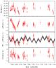 |
Fig. 1 Time series for, from top to bottom: a) the HARPS RVs of K2-3; b) ΔRV (Sect. 2.3); c) the RVs corrected from the αΔRV of the maximum likelihood model together with the dynamical model (the solid black line represents the median model, and the shades of grey represent the 68.3, 95.5, and 99.7% Bayesian confidence intervals); and d) the RV residual from the maximum likelihood dynamical model. |
Our results agree with Crossfield et al. (2015) for all parameters in common. In addition to adding the RV information, our analysis differs in that we neither impose a circular orbit nor use informative priors on R⋆/a or the limb darkening coefficient. We also model the transits of all three planets jointly rather than one planet at a time, enforcing consistency in the derived stellar properties. Our approach measures the stellar density more accurately than can be inferred from the average spectrum.
The times of the individual transit are measured with standard errors (which roughly translate to a 1σ detection limits for TTVs) of 1.4, 2.8, and 2.9 min for planets b, c, and d, respectively. Over the short time span of the HARPS observations, the RV of the dynamical model differs from that of a three-Keplerian model by at most 27 cm s-1, which is well below the ~ 2 m s-1 measurement noise.
Owing to the low eccentricities and almost edge-on inclinations, all three planets almost certainly undergo secondary eclipses. Table A.2 lists the epochs and durations of these secondary eclipses.
To evaluate the robustness of our mass measurements, we extended the RV by adding a linear drift, a fourth planet, a term proportional to the bisector of the spectra, and any combination of them. We also experimented with restricting the analysis to those RVs that seem unaffected by stellar activity (BJD−2 450 000 > 7070). They always produced similar velocity amplitudes (and masses) for Planet b, but a wide range of values for Planets c and d. We conclude that our data robustly measure the mass of Planet b, 8.4 ± 2.1 M⊕, but not those of c and d. Many more observations and very careful analysis will be needed to disentangle signatures of Planets c and d from the activity signal. Figure 2 shows the RV signal from Planet b after removing the other terms of the model.
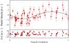 |
Fig. 2 HARPS RVs of K2-3 phased to the period of Planet b, with the Keplerian model (solid black line) overlaid, after removal of the Keplerians signals from Planets c and b and of αΔRV activity term of the maximum likelihood model. |
When included in the model, the fourth planet converges to a Pe ~ 100-day period and absorbs part of the residuals seen in Fig. 1 (bottom). Model comparison favours the four-planet model only marginally over the simpler three-planet model, with the Bayesian evidence estimators of Perrakis et al. (2014) and Chib & Jeliazkov (2001) giving odd ratios of 4.6 ± 0.3 and 4.9 ± 2.1, respectively, in favour of the four-planet model. More data will thus be needed to firmly establish whether additional planets orbit K2-3.
Figure 3 adds Planet b to the mass-radius diagram of the known small transiting planets. Planet b must contain rock with at most a 50% water envelope.
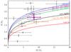 |
Fig. 3 Radius versus mass diagram of the known small exoplanets (Wright et al. 2011), with planet b added (magenta) with 68.3% credible intervals. The colored solid lines represents theoretical models for differents compositions (Zeng & Sasselov 2013). |
Planets around M stars are ideal for characterisation follow-up, thanks to the favourable planet-to-star surface ratio. The other known low-mass planets transiting bright M stars have a gas envelope (GJ436b and GJ3470b, Butler et al. 2004; Bonfils et al. 2012) or may even potentially consist of 100% water (GJ1214b, Charbonneau et al. 2009). Our measurement of the density of Planet b shows that it is either entirely rocky or mostly rocky with a water envelope. It is the first planet in this category, and the brightness of the star makes it a prime target for follow-up.
Online material
Appendix A: Additional figures and tables
HARPS RV measurements of K2-3.
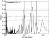 |
Fig. A.1 Periodogram of HARPS RVs of K2-3. The horizontal lines correspond to 1, 2, and 3σ confidence intervals. The false alarm probabilities (FAP) of the main peaks are 0.044% (20−30 days) and 0.0015% (8−10 days). The vertical lines indicate the period of Planets b, c, and d (from left to right). |
Model parameters: posterior mode and 68.3% credible intervals.
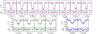 |
Fig. A.2 As in Fig. 1, but for the K2 photometry of K2-3 (from top to bottom and left to right: planet b, planet c, and planet d). Each transit is centered relative to the linear ephemeris. |
Acknowledgments
We thank the ESO La Silla staff for its continuous support, the HARPS observers (C. Mordasini, J. Martins, and A. Sozzetti, as well as L. Kreidberg for her Mandel & Agol code), C. Damiani for discussions of the dynamics of the system, and T. Fenouillet for his assistance with the LAM computing cluster. This paper includes data collected by the Kepler mission. Funding for the Kepler mission is provided by the NASA Science Mission directorate. Some of the data presented in this paper were obtained from the Mikulski Archive for Space Telescopes (MAST). STScI is operated by the Association of Universities for Research in Astronomy, Inc. under NASA contract NAS5-26555. Support for MAST for non-HST data is provided by the NASA Office of Space Science via grant NNX09AF08G and by other grants and contracts. This research made use of the Exoplanet Orbit Database and the Exoplanet Data Explorer at exoplanets.org. N.A.-D. acknowledges support from CONICYT Becas-Chile number 72120460. X.B. and J.M.A. acknowledge funding from the European Research Council under the ERC Grant Agreement No. 337591-ExTrA. NCS acknowledges support by Fundação para a Ciência e a Tecnologia (FCT) through Investigador FCT contracts of reference IF/00169/2012, and POPH/FSE (EC) by FEDER funding through the program “Programa Operacional de Factores de Competitividade – COMPETE”. A.S. is supported by the European Union under a Marie Curie Intra-European Fellowship for Career Development with reference FP7-PEOPLE-2013-IEF, number 627202. S.C.C.B. and O.D. thank the CNES for their grants 98761 and 124378, respectively.
References
- Anglada-Escudé, G., & Butler, R. P. 2012, ApJS, 200, 15 [NASA ADS] [CrossRef] [Google Scholar]
- Astudillo-Defru, N., Bonfils, X., Delfosse, X., et al. 2015, A&A, 575, A119 [NASA ADS] [CrossRef] [EDP Sciences] [Google Scholar]
- Barros, S. C. C., Almenara, J. M., Deleuil, M., et al. 2014, A&A, 569, A74 [NASA ADS] [CrossRef] [EDP Sciences] [Google Scholar]
- Bonfils, X., Gillon, M., Udry, S., et al. 2012, A&A, 546, A27 [NASA ADS] [CrossRef] [EDP Sciences] [Google Scholar]
- Bonfils, X., Delfosse, X., Udry, S., et al. 2013, A&A, 549, A109 [NASA ADS] [CrossRef] [EDP Sciences] [Google Scholar]
- Butler, R. P., Vogt, S. S., Marcy, G. W., et al. 2004, ApJ, 617, 580 [NASA ADS] [CrossRef] [Google Scholar]
- Chambers, J. E. 1999, MNRAS, 304, 793 [NASA ADS] [CrossRef] [MathSciNet] [Google Scholar]
- Charbonneau, D., Berta, Z. K., Irwin, J., et al. 2009, Nature, 462, 891 [NASA ADS] [CrossRef] [PubMed] [Google Scholar]
- Chib, S., & Jeliazkov, I. 2001, J. Am. Statist. Assoc., 96, 270 [Google Scholar]
- Crossfield, I. J. M., Petigura, E., Schlieder, J., et al. 2015, ApJ, 804, 1 [Google Scholar]
- Díaz, R. F., Almenara, J. M., Santerne, A., et al. 2014, MNRAS, 441, 983 [NASA ADS] [CrossRef] [Google Scholar]
- Fabrycky, D. C., Lissauer, J. J., Ragozzine, D., et al. 2014, ApJ, 790, 146 [NASA ADS] [CrossRef] [Google Scholar]
- Howell, S. B., Sobeck, C., Haas, M., et al. 2014, PASP, 126, 398 [NASA ADS] [CrossRef] [Google Scholar]
- Lovis, C., & Pepe, F. 2007, A&A, 468, 1115 [NASA ADS] [CrossRef] [EDP Sciences] [Google Scholar]
- Mandel, K., & Agol, E. 2002, ApJ, 580, L171 [NASA ADS] [CrossRef] [Google Scholar]
- Mayor, M., Pepe, F., Queloz, D., et al. 2003, The Messenger, 114, 20 [NASA ADS] [Google Scholar]
- Perrakis, K., Ntzoufras, I., & Tsionas, E. G. 2014, Comput. Statist. Data Anal., 77, 54 [Google Scholar]
- Stone, R. C. 1989, AJ, 97, 1227 [NASA ADS] [CrossRef] [Google Scholar]
- Vanderburg, A. 2014, ArXiv e-prints [arXiv:1412.1827] [Google Scholar]
- Vanderburg, A., & Johnson, J. A. 2014, PASP, 126, 948 [NASA ADS] [CrossRef] [Google Scholar]
- Vaughan, A. H., Preston, G. W., & Wilson, O. C. 1978, PASP, 90, 267 [NASA ADS] [CrossRef] [Google Scholar]
- Wright, J. T., Fakhouri, O., Marcy, G. W., et al. 2011, PASP, 123, 412 [NASA ADS] [CrossRef] [Google Scholar]
- Zeng, L., & Sasselov, D. 2013, PASP, 125, 227 [NASA ADS] [CrossRef] [Google Scholar]
- Zucker, S., & Mazeh, T. 2006, MNRAS, 371, 1513 [NASA ADS] [CrossRef] [Google Scholar]
All Tables
All Figures
|
Fig. 1 Time series for, from top to bottom: a) the HARPS RVs of K2-3; b) ΔRV (Sect. 2.3); c) the RVs corrected from the αΔRV of the maximum likelihood model together with the dynamical model (the solid black line represents the median model, and the shades of grey represent the 68.3, 95.5, and 99.7% Bayesian confidence intervals); and d) the RV residual from the maximum likelihood dynamical model. |
| In the text | |
|
Fig. 2 HARPS RVs of K2-3 phased to the period of Planet b, with the Keplerian model (solid black line) overlaid, after removal of the Keplerians signals from Planets c and b and of αΔRV activity term of the maximum likelihood model. |
| In the text | |
|
Fig. 3 Radius versus mass diagram of the known small exoplanets (Wright et al. 2011), with planet b added (magenta) with 68.3% credible intervals. The colored solid lines represents theoretical models for differents compositions (Zeng & Sasselov 2013). |
| In the text | |
|
Fig. A.1 Periodogram of HARPS RVs of K2-3. The horizontal lines correspond to 1, 2, and 3σ confidence intervals. The false alarm probabilities (FAP) of the main peaks are 0.044% (20−30 days) and 0.0015% (8−10 days). The vertical lines indicate the period of Planets b, c, and d (from left to right). |
| In the text | |
|
Fig. A.2 As in Fig. 1, but for the K2 photometry of K2-3 (from top to bottom and left to right: planet b, planet c, and planet d). Each transit is centered relative to the linear ephemeris. |
| In the text | |
Current usage metrics show cumulative count of Article Views (full-text article views including HTML views, PDF and ePub downloads, according to the available data) and Abstracts Views on Vision4Press platform.
Data correspond to usage on the plateform after 2015. The current usage metrics is available 48-96 hours after online publication and is updated daily on week days.
Initial download of the metrics may take a while.