| Issue |
A&A
Volume 581, September 2015
|
|
|---|---|---|
| Article Number | A53 | |
| Number of page(s) | 4 | |
| Section | Cosmology (including clusters of galaxies) | |
| DOI | https://doi.org/10.1051/0004-6361/201425431 | |
| Published online | 01 September 2015 | |
Research Note
Field equation of the correlation function of mass-density fluctuations for self-gravitating systems
Department of Astronomy, Key Laboratory for Researches in Galaxies and Cosmology, University of Science and Technology of China, Hefei, Anhui 230026, PR China
e-mail: This email address is being protected from spambots. You need JavaScript enabled to view it.
; This email address is being protected from spambots. You need JavaScript enabled to view it.
Received: 28 November 2014
Accepted: 1 July 2015
Abstract
We study the mass-density distribution of Newtonian self-gravitating systems. Modeling the system as a fluid in hydrostatical equilibrium, we obtain from first principles the field equation and its solution of the correlation function ξ(r) of the mass-density fluctuation itself. We apply this to studies of the large-scale structure of the Universe within a small redshift range. The equation shows that ξ(r) depends on the point mass m and the Jeans wavelength scale λ0, which are different for galaxies and clusters. It explains several long-standing prominent features of the observed clustering: that the profile of ξcc(r) of clusters is similar to ξgg(r) of galaxies, but with a higher amplitude and a longer correlation length, and that the correlation length increases with the mean separation between clusters as a universal scaling r0 ≃ 0.4d. Our solution ξ(r) also shows that the observed power-law correlation function of galaxies ξgg(r) ≃ (r0/r)1.7 is only valid in a range 1 <r< 10h-1 Mpc. At larger scales the solution ξ(r) breaks below the power law and goes to zero around ~50 h-1 Mpc, just as observational data have demonstrated. With a set of fixed model parameters, the solutions ξgg(r) for galaxies, the corresponding power spectrum, and ξcc(r) for clusters, simultaneously agree with the observational data from the major surveys of galaxies and clusters.
Key words: galaxies: clusters: general / large-scale structure of Universe / gravitation / cosmology: theory
© ESO, 2015
1. Introduction
It is one of the major goals of modern cosmology to understand the matter distribution in the Universe on large scales. The large-scale structure is determined by the self-gravity of galaxies and clusters. Since the number of galaxies is enormous, one needs statistics to study their distribution. In this regard, the two-point correlation functions ξgg(r) of galaxies and ξcc(r) clusters serve as a powerful statistical tool (Bok 1934; Totsuji & Kihara 1969; Peebles 1980). They not only provide statistical information, but also contain underlying dynamics that are mainly due to gravitational force. Therefore, we would like to investigate the correlation functions of self-gravitating systems in an approximation of hydrostatical equilibrium.
Over the years, various observational surveys have been carried out for galaxies and clusters, such as the Automatic Plate Measuring (APM) galaxy survey (Loveday et al. 1996), the Two-degree-Field Galaxy Redshift Survey (2dFGRS; Peacock et al. 2001), and the Sloan Digital Sky Survey (SDSS; Abazajian et al. 2009). All these surveys suggest that the correlation of galaxies has a power-law form ξgg(r) ∝ (r0/r)γ with r0 ~ 5.4h-1 Mpc and γ ~ 1.7 in a range (0.1 ~ 10)h-1 Mpc (Totsuji & Kihara 1969; Groth & Peebles 1977; Peebles 1980; Soneira & Peebles 1987). The correlation of clusters is found to be of a similar form: ξcc(r) ~ 20ξgg(r) in a range (5 ~ 60)h-1 Mpc, with an amplified magnitude (Bahcall & Soneira 1983; Klypin & Kopylov 1983). For quasars, the correlation is ξqq(r) ~ 5ξgg(r) (Shaver 1988). Numerical computations have been extensively employed to study clustering of galaxies and clusters, and significant progresses have been made. To understand physical mechanisms behind the clustering, analytical studies are important.
In particular, Saslaw (1985, 2000) used thermodynamics whereby the power-law form of ξgg(r) was introduced as modifications to the energy and pressure. Similarly, de Vega et al. (1996a,b, 1998) used the grand partition function of a self-gravitating gas to study a possible fractal structure of the distribution of galaxies. However, the field equation of ξ was not given in these studies. In this paper we set the speed of light to c = 1 and the Boltzmann constant to kB = 1.
2. Field equation of the two-point correlation function of density fluctuations
Galaxies or clusters that are distributed in the Universe can be described as fluids at rest in gravitational fields. This modeling is an approximation since cosmic expansion is not considered. We apply hydrostatics to systems of galaxies within a small redshift range. For these self-gravitating systems, the field equation of mass density is (Zhang 2007; Zhang & Miao 2009)  (1)where ψ(r) ≡ ρ(r) /ρ0 with ρ0 = mn0 is the mean mass density of the system,
  is the Jeans wave number, and J is a Schwinger type of external source introduced for taking the functional derivative (Schwinger 1951). The effective Hamiltonian density is
  (2)The generating functional for the correlation functions of ψ is
 ![Mathematical equation: \begin{equation} \label{ZJ} Z[J] = \int D\psi {\rm e}^{-\alpha \int d^{3}\vec{r}\mathcal{H}(\psi,J)}, \end{equation}](/articles/aa/full_html/2015/09/aa25431-14/aa25431-14-eq29.png) (3)where
(3)where  , cs is the sound speed and m is the mass of a single particle.
Since the distribution of galaxies or clusters can be viewed as fluctuations of the mass density in the Universe, we consider the fluctuation field δψ(r) ≡ ψ(r) − ⟨ ψ(r) ⟩, where the statistical ensemble average is defined as ![Mathematical equation: \hbox{$ \langle\psi(\vec{r})\rangle = \frac{\delta}{\alpha \delta J({\vec{r} })}\log Z[J] \mid_{J\,=\,0} $}](/articles/aa/full_html/2015/09/aa25431-14/aa25431-14-eq33.png) , and, in our case, ⟨ ψ(r) ⟩ = ψ0 is a constant. The connected n-point correlation function of δψ is defined as (Binney et al. 1992)
, and, in our case, ⟨ ψ(r) ⟩ = ψ0 is a constant. The connected n-point correlation function of δψ is defined as (Binney et al. 1992)  (4)for n ≥ 2. One can take G(2)(r1,r2) = G(2)(r12) for the homogeneous and isotropic Universe. To derive the field equation of G(2)(r) (Goldenfeld 1992), one takes functional derivative of the ensemble average of Eq. (1) with respect to J(r1). In doing this, G(3) occurs in the equation of G(2)(r) hierarchically. We adopt the Kirkwood-Groth-Peebles ansatz (Kirkwood 1932; Groth & Peebles 1977) G(3)(r1,r2,r3) = Q [ G(2)(r12)G(2)(r23) + G(2)(r23)G(2)(r31) + G(2)(r31)G(2)(r12) ] , where Q is a dimensionless parameter. Then, after a necessary renormalization, we obtain the field equation of the two-point correlation function
 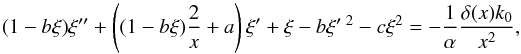 (5)where ξ = ξ(r) ≡ G(2)(r),
  , x ≡ k0r,
  , and a, b, and c are three independent parameters. Equation (5) extends that in our earlier work (Zhang & Miao 2009). The special case of a = b = c = 0 is the Gaussian approximation. The terms containing a, b, and c represent the nonlinear contributions beyond the Gaussian approximation. The nonlinear terms with b and c in Eq. (5) can enhance the amplitude of ξ at small scales and increase the correlation length. The term containing a plays the role of effective viscosity. The value of a should be high enough to ensure 1 + ξ(r) ≥ 0 for the whole range 0 <r< ∞.
3. General predictions of field equation
We inspect Eq. (5) to see its predictions on general properties of the correlation function ξ(r).
First, the equation contains a point mass m and a characteristic wave number k0. It applies to the system of galaxies and to the system of clusters, but with different m and k0 in each respective case. Thus, as solutions of Eq. (5), ξcc for clusters should have a profile similar to ξgg for galaxies, but will differ in amplitude and in scale determined by different m and k0. Indeed, the observations show that both ξgg and ξcc have a power-law form: ∝r-1.8 in their respective finite range, but ξcc has a higher amplitude (Bahcall & Soneira 1983; Klypin & Kopylov 1983).
Second, the δ3(r) source in Eq. (5) has a coefficient  , which determines the overall amplitude of a solution ξ. The mass m of a cluster can be 10 ~ 103 times that of a galaxy (Bahcall 1999), while cs regarded as the peculiar velocity is around several hundreds km s-1 for galaxies and clusters. Therefore, 1 /α ∝ m, and a greater m will yield a higher amplitude of ξ. This general prediction naturally explains a whole chain of prominent facts of observations: that luminous galaxies are more massive and have a higher correlation amplitude than ordinary galaxies (Zehavi et al. 2005), that clusters are much more massive and have a much higher correlation than galaxies, and that rich clusters have a higher correlation than poor clusters since richness is proportional to mass (Bahcall & Soneira 1983; Einasto et al. 2002, 2007; Bahcall et al. 2003). These phenomena have been a puzzle for long (Bahcall 1999) and were interpreted as being caused by the statistics of rare peak events (Kaiser 1984).
Third, the power spectrum is proportional to the inverse of the spatial number density: P(k) ∝ 1 /n0. Given the mean mass density ρ0 = mn0, a greater m implies a lower n0. Therefore, properties 2 and 3 reflect the same physical law of clustering from different perspectives. Property 3 also agrees with the observed fact from a variety of surveys. The observed P(k) of clusters is much higher than that of galaxies, and the observed P(k) of rich clusters is higher than poor clusters, etc. This is because the n0 of clusters is much lower than that of galaxies, and n0 of rich clusters is lower than that of poor clusters (Bahcall 1999).
Fourth, the characteristic length  appears in Eq. (5) as the only scale that underlies the scale-related features of clustering. Cluster surveys extend over larger spatial volumes, including those of highly diluted regions. The mass density ρ0c of the region covered by cluster surveys is lower than ρ0g for galaxy surveys, as implied in the references (Bahcall 1999; Bahcall et al. 1995). Thus, λ0 for cluster surveys will be longer than that for galaxy surveys. As we show in Sects. 4 and 5, in using one solution ξ(r) to match the data of both galaxies and clusters, one needs to take k0 smaller for clusters than for galaxies.
4. Comparing observational data of galaxy surveys
Now we give the solution ξgg(r) for a fixed set of parameters (a,b,c) and compare the observed correlation from major galaxy surveys.
First we consider the correlation function ξgg(r).
Figure 1 shows the solution ξgg(r) and the observational data by the galaxy surveys of APM (Padilla & Baugh 2003), SDSS (Zehavi et al. 2005), and 2dFGRS (Hawkins et al. 2003). The theoretical ξgg(r) matches the data in the range of r = (2 ~ 50)h-1 Mpc. The usual power-law ξgg ∝ r-1.7 is only valid in an interval (0.1 ~ 10)h-1 Mpc. On large scales, the solution ξgg(r) deviates from the power law, rapidly decreases to zero, and becomes negative around 50h-1 Mpc. However, on small scales r ≤ 1h-1 Mpc, the solution ξgg(r) is lower than the data, even though it has already improved the Gaussian approximation (Zhang 2007). This insufficiency at r ≤ 1h-1 Mpc is probably due to neglect of high-order nonlinear terms such as (δψ)3 in our perturbation. We remark that the equation of ξgg(r) has been derived assuming δψ< 1. Thus, it is only an approximation to extrapolate our calculated ξgg(r) down to smaller scales r ≤ 5h-1 Mpc.
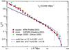 |
Fig. 1 Solution ξgg(r) compares the data of galaxies by APM (Padilla & Baugh 2003), 2dFGRS (Hawkins et al. 2003), and SDSS (Zehavi et al. 2005). Here k0 = 0.055h Mpc-1 is included in the calculation. |
We verified that the approximation of hydrostatical equilibrium can be applied in the quasi-linear regime in the expanding Universe. The density fluctuation approximately behaves as δψ ∝ a(t)0.3, where a(t) is the scale factor in the present stage of accelerating expansion. So the time-evolving correlation function ξgg(r,t) = ⟨ δψδψ ⟩ ∝ a0.6(t) = 1 / (1 + z)0.6. For the sample of ~200 000 galaxies of the SDSS (Zehavi et al. 2005), the redshift range is z = (0.02 ~ 0.167). Taking its maximum z = 0.167 into the ratio gives ξgg(r) /ξgg(r,t) ≃ (1 + 0.167)0.6 ~ 1.097, and the error is 0.6z ≃ 0.1. The conclusion of this analysis has also been supported by studies of numerical simulations (Hamana et al. 2001; Yoshikawa et al. 2001; Taruya et al. 2001).
Then we consider the power spectrum P(k). The power spectrum P(k) is the Fourier transform  (6)of the correlation function ξ(r). It measures the mass-density fluctuation in k-space. In principle, P(k) and ξ(r) contain the same information if both are complete in their respective space, k = (0,∞), and r = (0,∞). The observed ξgg(r) is not complete, however, because it is limited to a finite range, for example, r ≤ 50 Mpc. If the observed power-law ξgg(r) = (r0/r)1.8 were plugged into Eq. (6), one would have P(k) ∝ k-1.2, which does not comply with the observed P(k) ∝ k-1.6 (Peacock 1999). Our P(k) is obtained from the solution ξgg(r) given on the whole range r = (0,∞). Figure 2 shows the theoretical P(k) converted by Eq. (6) from the solution ξgg(r) with the same set (a,b,c) and k0 as those in Fig. 1. We also show in Fig. 2 the observational data of P(k) from APM (Padilla & Baugh 2003), 2dFGRS (Cole et al. 2005), and SDSS (Blanton et al. 2004). The theoretical P(k) agrees well with the data P(k) ∝ k-1.6 in the range of k = (0.04 ~ 0.7) h Mpc-1. However, at large k, the theoretical P(k) is lower than the data. This insufficiency of P(k) corresponds to that of ξgg(r) at small scales r ≤ 1h-1 Mpc shown in Fig. 1.
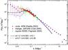 |
Fig. 2 Power spectrum P(k) converted from ξgg(r) in Fig. 1 compares the data of APM (Padilla & Baugh 2003), 2dFGRS (Cole et al. 2005), and SDSS (Blanton et al. 2004). |
5. Comparing the observational data of clusters
Clusters are believed to trace the cosmic mass distribution on even larger scales, and the observational data cover spatial scales that exceed those of galaxies. Now we apply the solution with the same two sets of (a,b,c) as in Sect. 4 to the system of clusters. A cluster has a mass m greater than that of a galaxy. This leads to a higher overall amplitude of ξcc(r). In addition, to match the observational data of clusters, a low value k0 = 0.03 Mpc-1 is required, lower than that for galaxies.
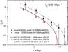 |
Fig. 3 Solution ξcc(r) for clusters compares the data of SDSS clusters of two types of richness (Bahcall et al. 2003). Here (a,b,c) are the same for galaxies. But k0 = 0.03h Mpc-1 is taken for clusters, smaller than that for galaxies. |
For each set of values of (a,b,c), two solutions ξcc(r) with different amplitudes are given in Fig. 2 and are compared with two sets of data of richness N> 10 and N> 20 from the SDSS (Bahcall et al. 2003). Interpreted by Eq. (5), the N> 20 clusters have a greater m than the N> 10 clusters. The solutions match the data in the whole range r = (4 ~ 100)h-1 Mpc.
It has long been known that there is a scaling behavior of cluster correlation. The correlation scale increases with the mean spatial separation between clusters (Szalay & Schramm 1985; Bahcall & West 1992; Bahcall 1999; Croft et al. 1997; Gonzalez et al. 2002). If a power law ξcc = (r0/r)1.8 were used to fit the data, the “correlation length” would be of a form r0 ≃ 0.4di, where  and ni is the mean number density of clusters of type i. Simulations have also produced this r0 − di dependence (Bahcall & Cen 1992). For SDSS, the scaling can also be fitted by r0 ≃ 2.6di1 / 2 (Bahcall et al. 2003) and for the 2df galaxy groups by r0 ≃ 4.7di0.32 (Zandivarez et al. 2003). This kind of universal scaling of r0 − di has been a theoretical challenge (Bahcall 1997), and was thought to be either caused by a fractal distribution of galaxies and clusters (Szalay & Schramm 1985) or by the statistics of rare peak events (Kaiser 1984). The difference in the scaling slope was attributed to the different richness of clusters (Bahcall 1997). In our theory the scaling is fully embodied in the solution ξcc(k0r) with the characteristic wave number
  . To comply with the empirical power-law, we take the theoretical “correlation length” as
  , where ξcc is the theoretical solution and depends on d. Figure 4 shows that the solution ξcc with k0 = 0.03h Mpc-1 gives the universal scaling r0(d) ≃ 0.4d, which agrees well with the observation (Bahcall 1999). If a greater k0 = 0.055h Mpc-1 is taken, the solution ξcc would yield a flatter scaling r0(d) ≃ 0.3d, which better fits the data of APM clusters (Bahcall et al. 2003). Our analysis based on the solution ξcc reveals that a higher background density ρ0 predicts a flatter slope of the scaling r0(d). To conclude, the universal r0 − di scaling is naturally explained by the solution ξcc(r).
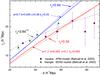 |
Fig. 4 Solution ξcc(r) with k0 = 0.03h Mpc-1 gives the universal scaling r0 ≃ 0.4d. If a greater k0 = 0.055h Mpc-1 is taken, ξcc would give a flatter scaling r0 ≃ 0.3d, which better fits the data of APM clusters (Bahcall et al. 2003). |
6. Conclusions and discussions
We have presented a field theory of density fluctuations of Newtonian gravitating systems and applied it to the study of correlation functions of galaxies and clusters. We obtained the field equation Eq. (5) of the two-point correlation function as a main result by starting from the field equation Eq. (1) of mass density, under the condition of hydrostatic equilibrium and keeping to the nonlinear order of (δψ)2 in perturbation, by taking the functional derivative. In deriving Eq. (5), we adopted the Kirkwood-Groth-Peebles ansatz necessary to cut off the hierarchy in n-point correlation functions and renormalized this to absorb divergences into the parameters. This analytic approach from first principles is different from those using gravitational potential. Equation (5) clearly explains the observational data of clustering of galaxies and clusters
on large scales. To extend the analytic study further, higher-order nonlinear terms should be included to describe small-scale clusterings better, and the cosmic evolution should be taken into consideration as a more realistic model.
Acknowledgments
Y. Zhang is supported by NSFC No. 11275187, NSFC 11421303, SRFDP, and CAS, the Strategic Priority Research Program “The Emergence of Cosmological Structures” of the Chinese Academy of Sciences, Grant No. XDB09000000.
References
- Abazajian, K. N., Adelman-McCarthy, J. K., Agüeros, M. A., et al. 2009, ApJS, 182, 543 [NASA ADS] [CrossRef] [Google Scholar]
- Bahcall, N. A. 1997, in Unsolved Problems in Astrophysics, eds. J. N. Bahcall, & J. P. Ostriker (Princeton University Press), 61 [Google Scholar]
- Bahcall, N. A. 1999, in Formation of Structure in the Universe, eds. A. Dekel, & J. P. Ostriker (Cambridge University Press), 135 [Google Scholar]
- Bahcall, N. A., & Cen, R. 1992, ApJ, 398, L81 [NASA ADS] [CrossRef] [Google Scholar]
- Bahcall, N. A., & Soneira, R. M. 1983, ApJ, 270, 20 [NASA ADS] [CrossRef] [Google Scholar]
- Bahcall, N. A., & West, M. 1992, ApJ, 392, L419 [NASA ADS] [CrossRef] [Google Scholar]
- Bahcall, N. A., Lubin, L. M., & Dorman, V. 1995, ApJ, 447, L81 [NASA ADS] [CrossRef] [Google Scholar]
- Bahcall, N. A., Dong, F., Hao, L., et al. 2003, ApJ, 599, 814 [NASA ADS] [CrossRef] [Google Scholar]
- Binney, J. J, Dowrick, N., Fisher, A., & Newman, M., 1992, The Theory of Critical Phenomena (Oxford University Press) [Google Scholar]
- Blanton, M., Tegmark, M., & Strauss, M. 2004, ApJ, 606, 702 [NASA ADS] [CrossRef] [Google Scholar]
- Bok, B. J. 1934, Bull Harvard Obs, 895, 1 [NASA ADS] [Google Scholar]
- Cole, S., Percival, W. J., Peacock, J. A., et al. 2005, MNRAS, 362, 505 [NASA ADS] [CrossRef] [Google Scholar]
- Croft, R. A. C., Dalton, G. B., Efstathiou, G., Sutherland, W. J., & Maddox, S. J., 1997, MNRAS, 291, 305 [NASA ADS] [CrossRef] [Google Scholar]
- de Vega, H. J., Sanchez, N., & Combes, F., 1996a, Phys. Rev. D, 54, 6008 [NASA ADS] [CrossRef] [Google Scholar]
- de Vega, H. J., Sanchez, N., & Combes, F., 1996b, Nature, 383, 56 [NASA ADS] [CrossRef] [Google Scholar]
- de Vega, H. J., Sanchez, N., & Combes, F. 1998, ApJ, 500, 8 [NASA ADS] [CrossRef] [Google Scholar]
- Einasto, M., Einasto, J., Tago, E., Andernach, H., Dalton, G. B., & Müller, V. 2002, AJ, 123, 51 [NASA ADS] [CrossRef] [Google Scholar]
- Einasto, M., Einasto, J., Tago, E., et al. 2007, ApJ, 123, 51 [Google Scholar]
- Goldenfeld, N. 1992, Lectures on Phase Transitions and Renormalization Group (Addison-Wesley Publishing Company) [Google Scholar]
- Gonzalez, A. H., Zaritsky, D., & Wechler, R. H. 2002, ApJ, 571, 129 [NASA ADS] [CrossRef] [Google Scholar]
- Groth, E., & Peebles, P. J. E. 1977, ApJ, 217, 385 [NASA ADS] [CrossRef] [Google Scholar]
- Hamana, T., Colombi, S., & Suto, Y. 2001, A&A, 367, 18 [NASA ADS] [CrossRef] [EDP Sciences] [Google Scholar]
- Hawkins, E., Maddox, S., Cole, S., et al. 2003, MNRAS, 346, 78 [Google Scholar]
- Kaiser, N. 1984, ApJ, 284, L9 [NASA ADS] [CrossRef] [Google Scholar]
- Kirkwood, J. G. 1932, J. Chem. Phys., 3, 300 [Google Scholar]
- Klypin, A. A., & Kopylov, A. I. 1983, Sov. Astron. Lett., 9, 41 [NASA ADS] [Google Scholar]
- Loveday, J., Peterson, B. A., Maddox, S. J., & Efstathiou, G. 1996, ApJS, 107, 201 [NASA ADS] [CrossRef] [Google Scholar]
- Masters, K. L., Springob, C. M., Haynes, M. P., & Giovanelli, R. 2006, ApJ, 653, 861 [NASA ADS] [CrossRef] [Google Scholar]
- Padilla, N. D., & Baugh, C. M. 2003, MNRAS, 343, 796 [NASA ADS] [CrossRef] [Google Scholar]
- Peacock, J. A. 1999, Cosmological Physics (Cambridge, UK: Cambridge Univ. Press) [Google Scholar]
- Peacock, J., Cole, S., Norberg, P., et al. 2001, Nature, 410, 169 [NASA ADS] [CrossRef] [PubMed] [Google Scholar]
- Peebles, P. J. E. 1980, The Large-scale Structure of the Universe (Princeton, NJ: Princeton Univ. Press) [Google Scholar]
- Saslaw, W. C. 1985, Gravitational Physics of Stellar and Galactic Systems (Cambridge University Press) [Google Scholar]
- Saslaw, W. C. 2000, The Distribution of the Galaxies (Cambridge University Press) [Google Scholar]
- Schwinger, J. 1951, PNAS, 37, 452 [Google Scholar]
- Shaver, P. 1988, in Large-Scale Structure of the Universe, eds. J. Audouze, et al. (Dordrecht: Reidel), IAU Symp. 130, 359 [Google Scholar]
- Soneira, R. M., & Peebles, P. J. E. 1987, AJ, 83, 845 [Google Scholar]
- Szalay, A., & Schramm, D. 1985, Nature, 314, 718 [NASA ADS] [CrossRef] [Google Scholar]
- Taruya, A., Magira, H., Jing, Y. P., & Suto, Y. 2001, PASJ, 53, 155 [NASA ADS] [Google Scholar]
- Totsuji, H., & Kihara, T. 1969, PASJ, 21, 221 [NASA ADS] [Google Scholar]
- Yahata, K., Suto, Y., Kayo, I., et al. 2005, PASJ, 57, 529 [NASA ADS] [Google Scholar]
- Yoshikawa, K., Taruya, A., Jing, Y. P., & Suto, Y. 2001, ApJ, 558, 520 [NASA ADS] [CrossRef] [Google Scholar]
- Zandivarez, A., Merchan, M. E., & Padilla, N. D. 2003, MNRAS, 344, 247 [NASA ADS] [CrossRef] [Google Scholar]
- Zehavi, I., Zheng, Z., & Weinberg, D. H., et al. 2005, ApJ, 630, 1 [Google Scholar]
- Zhang, Y. 2007, A&A, 464, 811 [NASA ADS] [CrossRef] [EDP Sciences] [Google Scholar]
- Zhang, Y., & Miao, H. X. 2009, RA&A, 9, 501 [Google Scholar]
All Figures
|
Fig. 1 Solution ξgg(r) compares the data of galaxies by APM (Padilla & Baugh 2003), 2dFGRS (Hawkins et al. 2003), and SDSS (Zehavi et al. 2005). Here k0 = 0.055h Mpc-1 is included in the calculation. |
| In the text | |
|
Fig. 2 Power spectrum P(k) converted from ξgg(r) in Fig. 1 compares the data of APM (Padilla & Baugh 2003), 2dFGRS (Cole et al. 2005), and SDSS (Blanton et al. 2004). |
| In the text | |
|
Fig. 3 Solution ξcc(r) for clusters compares the data of SDSS clusters of two types of richness (Bahcall et al. 2003). Here (a,b,c) are the same for galaxies. But k0 = 0.03h Mpc-1 is taken for clusters, smaller than that for galaxies. |
| In the text | |
|
Fig. 4 Solution ξcc(r) with k0 = 0.03h Mpc-1 gives the universal scaling r0 ≃ 0.4d. If a greater k0 = 0.055h Mpc-1 is taken, ξcc would give a flatter scaling r0 ≃ 0.3d, which better fits the data of APM clusters (Bahcall et al. 2003). |
| In the text | |
Current usage metrics show cumulative count of Article Views (full-text article views including HTML views, PDF and ePub downloads, according to the available data) and Abstracts Views on Vision4Press platform.
Data correspond to usage on the plateform after 2015. The current usage metrics is available 48-96 hours after online publication and is updated daily on week days.
Initial download of the metrics may take a while.