| Issue |
A&A
Volume 580, August 2015
|
|
|---|---|---|
| Article Number | A123 | |
| Number of page(s) | 7 | |
| Section | Astrophysical processes | |
| DOI | https://doi.org/10.1051/0004-6361/201526242 | |
| Published online | 17 August 2015 | |
Comparative study of a constant-alpha force-free field and its approximations in an ideal toroid
1
Astronomical Institute, Academy of Sciences of the Czech
Republic, Boční II
1401, 141 00
Praha 4, Czech
Republic
e-mail:
This email address is being protected from spambots. You need JavaScript enabled to view it.
2
Lone Star College, Houston, TX77088
Texas,
USA
e-mail:
This email address is being protected from spambots. You need JavaScript enabled to view it.
Received: 2 April 2015
Accepted: 19 June 2015
Abstract
Aims. Magnetic clouds in the solar wind are large, loop-like interplanetary flux ropes and may be locally approximated by a toroidal flux rope. We compare approximate constant-alpha force-free fields in an ideal toroid, used in magnetic cloud analysis, with the exact solution, and examine their validity for low aspect ratios, which can be found in magnetic clouds. The approximate toroidal solutions were originally derived under the assumption of large aspect ratios.
Methods. Three analytic simple approximate constant-alpha force-free solutions and the exact analytic solution are compared with respect to magnetic field profiles, magnetic field magnitude distributions, and magnetic helicity, with moderate (2–3) and very low (<2) aspect ratios.
Results. The Miller & Turner (1981, Phys. Fluids, 24, 363) field and its modification (to satisfy exact solenoidality) match the position of the magnetic axis in the toroidal flux rope well even for very low aspect ratios. The same can be said for the modified field and the position of the magnetic field maximum. When calculating helicity of the toroidal flux rope, the Miller & Turner field yields better results. A simple formula for magnetic helicity derived from the Miller & Turner solution is valid with a good accuracy even for very low aspect ratios.
Conclusions. The Miller & Turner solution is a reasonable substitute for the exact solution even for low aspect ratios (≈2).
Key words: solar wind / magnetic fields / magnetohydrodynamics (MHD)
© ESO, 2015
1. Introduction
It is widely accepted that magnetic flux ropes are quite commonly observed in the solar wind. Their first in-situ observations were reported during the 1970s (Krimigis et al. 1976). Large and relatively cold interplanetary flux ropes were labelled magnetic clouds (Burlaga et al. 1981; Klein & Burlaga 1982; Burlaga & Behannon 1982), and their relationship to coronal mass ejections coming from the Sun was found (Burlaga et al. 1982). More detailed examinations revealed that, aside from magnetic clouds, there were many smaller-scale flux ropes present in the solar wind (Shimazu & Marubashi 2000; Moldwin et al. 2000; Mandrini et al. 2005; Cartwright & Moldwin 2010). Burlaga (1988) suggested using a simple constant-alpha force-free field in a cylindrical flux rope (derived by Lundquist 1950) to model a magnetic field configuration inside magnetic clouds. This configuration proved to be very useful for the evaluation of magnetic cloud parameters (e.g. axis orientation, radius, helicity) and, within this model, these parameters are nearly routinely estimated for all identified magnetic clouds (cf. Lepping et al. 1990, 2006, 2015), as well as in some small-scale flux-rope studies (e.g. Shimazu & Marubashi 2000).
It is evident that modelling an interplanetary-flux-rope magnetic configuration by a cylindrical flux rope can only be done locally. Interplanetary flux ropes are bent and, at least for some time, they remain connected by their feet to the Sun (Burlaga et al. 1990; Chen & Garren 1993; Marubashi 1997; Janvier et al. 2013). In some cases curvature of flux ropes must be taken into account to correctly interpret magnetic field observations inside interplanetary flux ropes (Ivanov et al. 1989; Marubashi 1997; Romashets & Vandas 2003a; Marubashi & Lepping 2007; Hidalgo 2014). Usually it is a local fitting because the model is an ideal torus. Hidalgo (2013, 2014) recently published a global model of an interplanetary flux rope, which has a varying cross section and a non-circular axis. It is a non-force-free model. In the present paper, we deal with linear force-free configurations. In that case, a flux rope is locally modelled by an ideal toroid either with a toroidally adjusted Lundquist solution (Marubashi 1997), or with the Miller & Turner (1981) solution (Ivanov et al. 1989). Toroidally adjusted Lundquist solution is a very rough approximation and the Miller and Turner solution was derived under an assumption of large aspect ratios (the ratios between the major, R0, and minor, r0, radii of a toroid). Geometrical considerations (Marubashi 1997) or magnetohydrodynamic simulations (Vandas et al. 2002) indicate that there are bent parts of interplanetary flux ropes where the curvature is quite high, and hence aspect ratios are relatively low. It raises the question of whether these parts can be meaningfully fitted by the above mentioned solutions, however, Tsuji (1991) proposed the solution of a linear force-free configuration in an ideal toroid of an arbitrary aspect ratio, which is not widely known in the space-research community. In the next section, we describe this solution and list approximate linear force-free toroidal solutions used for interpretation of magnetic cloud observations. The Tsuji solution is computationally expensive and not very easy to implement in comparison with the approximate solutions, which are very simple. Therefore, for practical reasons the approximate solutions would be preferred, and we check here how they compare with the exact solution, especially for lower aspect ratios. Some preliminary comparisons have been made in our proceeding papers (Romashets & Vandas 2003b; Vandas & Romashets 2010), and here we present more comprehensive comparisons, with special emphasis on magnetic helicity when aspect ratio is moderate or very low. Validity of a simple analytic formula for helicity, derived from the Miller and Turner solution, is examined for low aspect ratios.
2. Toroidal constant-alpha force-free models
Linear force-free field B fulfills the condition  (1)where α is a constant (α ≠ 0), hence this force-free field is also called a constant-alpha force-free field. The sign of α determines the chirality of the field. Applying div operator to Eq. (1), we see that the field is automatically solenoidal.
The Lundquist (1950) linear force-free field in a cylindrical flux rope, given in cylindrical coordinates r, ϕ, and Z, reads  where Jn are the Bessel functions of the first kind, B0 scales the magnetic field and it is also the value of the field maximum located at the flux rope axis (r = 0). Each r = const. is a magnetic surface, hence, each cylinder may form a flux rope. The component BZ reaches its maximum at the axis and then monotonously decreases to zero at αr = a0, where a0 is the first root of J0 (a0 ≈ 2.405). Usually, the flux rope boundary is set at this place, so α is related to the flux rope radius r0 by
  (5)The toroidally adjusted Lundquist solution simply results from an ad-hoc change of field components in cylindrical coordinates into toroidally curved cylindrical coordinates r, ϕ, and θ (Fig. 1a),
  and it reads
  One cannot expect that this field to be solenoidal or force-free. The boundary of our toroid is determined by r = r0, 0 ≤ θ ≤ 2π, 0 ≤ ϕ ≤ 2π, and its volume by 0 ≤ r ≤ r0, 0 ≤ θ ≤ 2π, 0 ≤ ϕ ≤ 2π.
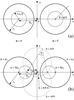 |
Fig. 1 Two coordinate systems shown separately in a) and b), that we used for descriptions of toroidal magnetic field configurations. Cross sections of our toroid’s surface (with major and minor radii, R0 and r0, respectively) with the xz plane are shown with the thick circles. Our toroid has a circular axis at |

The Miller & Turner (1981) solution was derived under assumption of a large aspect ratio R0/r0 of a toroid and in its simplest form, used in magnetic cloud analyses, it reads ![Mathematical equation: \begin{eqnarray} \label{MTBr}B_r^\mathrm{(MT)} & = & \frac{B_0}{2 \alpha R_0} {J}_0(\alpha r) \sin \theta , \\ \label{MTBp}B_\varphi^\mathrm{(MT)} & = & B_0 \left( 1 - \frac{r}{2 R_0} \cos \theta \right) {J}_0(\alpha r) , \\ \label{MTBt}B_\theta^\mathrm{(MT)} & = & - B_0 \left\{{J}_1(\alpha r) - \frac{1}{2 \alpha R_0} \left[{J}_0(\alpha r) + \alpha r {J}_1(\alpha r)\right] \cos \theta \right\} . \quad\quad\quad \end{eqnarray}](/articles/aa/full_html/2015/08/aa26242-15/aa26242-15-eq49.png) The Miller & Turner solution is not exactly solenoidal. We tried to fix this problem (Romashets & Vandas 2003b) and suggested a modified Miller & Turner solution, derived via the magnetic vector potential. The magnetic vector potential A is defined by
The Miller & Turner solution is not exactly solenoidal. We tried to fix this problem (Romashets & Vandas 2003b) and suggested a modified Miller & Turner solution, derived via the magnetic vector potential. The magnetic vector potential A is defined by  (15)and can be easily specified for a linear force-free field by
  (16)because rot A = rot B/α = B. Strictly speaking, the magnetic vector potential of the Miller & Turner solution does not exist because this field is not exactly solenoidal. Hence, the expression B(MT)/α from Eq. (16) is not the magnetic vector potential of the Miller & Turner solution in an exact sense, but we regard it as a magnetic vector potential of a field, which we call the modified Miller & Turner (mMT) solution,
  (17)so the modified Miller & Turner solution can be expressed as
  (18)explicitly,
 ![Mathematical equation: \begin{eqnarray} B^\mathrm{(mMT)}_r & = & B_0 \frac{R_0 - 2 r \cos \theta} {2 \alpha R_0 (R_0 + r \cos \theta)} {J}_0(\alpha r) \sin \theta , \label{mMTBr} \\ B^\mathrm{(mMT)}_\varphi & = & B_0 \left( 1 - \frac{r}{2 R_0} \cos \theta \right) {J}_0(\alpha r) , \label{mMTBp} \\ B^\mathrm{(mMT)}_\theta & = & - \frac{B_0}{2 \alpha R_0 (R_0 + r \cos \theta)} \bigg\{2 \alpha R_0^2 {J}_1(\alpha r) \nonumber \\ & & -\ R_0 \left[{J}_0(\alpha r) - \alpha r {J}_1(\alpha r)\right] \cos \theta \nonumber \\ & & +\ r \left[2 {J}_0(\alpha r) - \alpha r {J}_1(\alpha r)\right] \cos^2 \theta\bigg\} . \label{mMTBt} \end{eqnarray}](/articles/aa/full_html/2015/08/aa26242-15/aa26242-15-eq57.png) For large aspect ratios, the Miller & Turner solution is close to a linear force-free field, so the modified Miller & Turner solution is close to the Miller & Turner solution because of the definition (18). In addition, the modified Miller & Turner solution is exactly solenoidal for any aspect ratio because div B(mMT) = div rot A(mMT) = 0 (as every field defined by a vector potential).
For large aspect ratios, the Miller & Turner solution is close to a linear force-free field, so the modified Miller & Turner solution is close to the Miller & Turner solution because of the definition (18). In addition, the modified Miller & Turner solution is exactly solenoidal for any aspect ratio because div B(mMT) = div rot A(mMT) = 0 (as every field defined by a vector potential).
These three toroidal solutions have Br = 0 at the toroid’s boundary r = r0 when α is given by Eq. (5), and so their magnetic field configurations are confined into an ideal toroid (with circular cross section), they are axisymmetric (with respect to the rotational axis (z), i.e. the fields do not depend on ϕ), their axial fields (Bϕ) are zero at the boundary, and they tend to the Lundquist solution for large aspect ratios (R0/r0 → ∞). In that sense, they represent a toroidal counterpart of the Lundquist solution. However, they are only approximately force-free: with accuracy expressed in r0/R0, this condition is fulfilled as  in case of the toroidally adjusted Lundquist solution and as
  for the Miller & Turner and modified Miller & Turner solutions; and the same holds for accuracy of solenoidality for the first two solutions (Romashets & Vandas 2003b; Vandas & Romashets 2010). The genuine toroidal counterpart of the Lundquist solution follows from the Tsuji (1991) solution. This solution is formulated for a general cross section and it was not very easy to extract our case from the given paper. We find it useful to present this special case here in a form enabling a straightforward implementation available for magnetic cloud or other research. The solution is exactly solenoidal and force-free for any aspect ratio.
The Tsuji solution is given in toroidal coordinates μ, η, and ϕ (Fig. 1b) determined by the following relationships to Cartesian coordinates:  The parameter a> 0 scales the system. Each coordinate μ = const.> 0 represents a surface of a toroid (while μ ≥ 0 in general). When
  , then our toroid has μ = μ0, coshμ0 = R0/r0. The angle ϕ is an azimuthal (rotational) angle of the toroid, ϕ ∈ ⟨ 0,2π), and the angle η ∈ ⟨ −π,π ⟩ complements the coordinates. The boundary of our toroid is determined by μ = μ0, −π ≤ η ≤ π, 0 ≤ ϕ ≤ 2π, and its volume by μ ≥ μ0, −π ≤ η ≤ π, 0 ≤ ϕ ≤ 2π.
The field is  with the Lamé coefficients
  (28)and
  (29)where
  (30)with
  (31)gl and
  are coefficients. The latter coefficients are fixed and they are given in Appendix A with some remarks on calculation procedures.
The coefficients gl are determined by the boundary condition, i.e. for us  at μ = μ0. The component
  from Eq. (25) explicitly is
  (32)The coefficient g0 is arbitrary (scales the field) and can be set equal to 1. The functions
  (n ≥ 0) are constants at the boundary and we denote
  . Writing Eq. (32) for the boundary and realizing that it must be fulfilled for every η, we get
  (33)This is a set of equations for gl.
In previous cases, α was simply related to the flux rope size by Eq. (5). It resulted from the second requirement, axial field to be zero at the boundary, here  at μ = μ0. Using Eq. (27) and utilizing Eq. (33), we get
  (34)This is an implicit equation for α.
In fact, Eqs. (33) and (34) are intertwined and must be solved simultaneously. In practice, the summation is cut at some L. Equation (34) is solved by a root finding method (we used bi-section method, Press et al. 2002). For a given α, the formula (33) represents a set of linear equations for gl, l = 1,...,L, to be solved by a numerical method (we used singular value decomposition method, Press et al. 2002). With gl evaluated, α is checked if it fulfills Eq. (34) to a specified accuracy. For large aspect ratios, | α | r0 should go to a0. Figure 2 shows how | α | r0 depends on the aspect ratio (cf. with Fig. 6 in Tsuji 1991). Some values are also tabulated in Table 1.
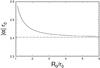 |
Fig. 2 Dependence of the force-free constant α on the aspect ratio R0/r0 of a toroid. For large aspect ratios, it tends to an asymptotic value, shown with the dashed-dotted line, which is consistent with the Lundquist solution. It is the first root of the Bessel function J0, a0. |
Alpha as a function of aspect ratio.
Magnetic helicity is defined for a magnetically closed body (which our toroid is) and it is given by  (35)where integration is over the body volume V (in our case the toroid with μ = μ0). For a linear force-free field, it simplifies into
  (36)where B is the magnetic field magnitude. The helicity for the Tsuji solution (25)–(27) must be calculated numerically. For the other solutions presented here, it can be evaluated analytically.
Using Eq. (36), the calculation for the Miller & Turner solution yields ![Mathematical equation: \begin{eqnarray} H^\mathrm{(MT)} & = & \frac{2 \pi}{\alpha} \, \int\limits_0^{2 \pi} \int\limits_0^{r_0} B^2 \, r (R_0 + r \cos \theta) \, \mathrm{d}r \, \mathrm{d}\theta \nonumber \\ & = & \frac{B_0^2 \pi^2 r_0^3 R_0}{2 a_0} \left[8-\left(1+\frac{1}{a_0^2} \right) \frac{r_0^2}{R_0^2}\right] {J}_1^2(a_0) \, \mathrm{sign} \, \alpha \label{HMT} , \end{eqnarray}](/articles/aa/full_html/2015/08/aa26242-15/aa26242-15-eq100.png) (37)where sign is the signum function. Because the magnetic field is only approximately force-free, the helicity H(MT) given by Eq. (37) is also only approximate and valid for larger aspect ratios. The helicity per unit length is given by
(37)where sign is the signum function. Because the magnetic field is only approximately force-free, the helicity H(MT) given by Eq. (37) is also only approximate and valid for larger aspect ratios. The helicity per unit length is given by ![Mathematical equation: \begin{equation} \label{HMTl} H^\mathrm{(MT)}_l = \frac{H^\mathrm{(MT)}}{2 \pi R_0} = \frac{B_0^2 \pi r_0^3}{4 a_0} \left[8-\left(1+\frac{1}{a_0^2} \right) \frac{r_0^2}{R_0^2}\right] {J}_1^2(a_0) \, \mathrm{sign} \, \alpha , \end{equation}](/articles/aa/full_html/2015/08/aa26242-15/aa26242-15-eq103.png) (38)which reduces for large aspect ratios into
(38)which reduces for large aspect ratios into  (39)The magnetic helicity for the modified Miller & Turner solution is given by
 ![Mathematical equation: \begin{equation} \label{HmMT} H^\mathrm{(mMT)} = \frac{B_0^2 \pi^2 r_0^3 R_0}{2 a_0} \left[8-\left(1- \frac{2}{a_0^2} \right) \frac{r_0^2}{R_0^2}\right] {J}_1^2(a_0) \, \mathrm{sign} \, \alpha . \end{equation}](/articles/aa/full_html/2015/08/aa26242-15/aa26242-15-eq105.png) (40)Equation (35) was used for the calculation because we know both the field (18) and its vector potential (17). The helicity (40) is exact. The helicity per unit length for large aspect ratios coincides with Eq. (39). The value in this equation also is the helicity per unit length for the toroidally adjusted Lundquist solution (that is, it does not depend on the aspect ratio in this case). A cylindrical flux rope is not a closed finite volume. Instead of helicity, the relative helicity per unit length is used for cylindrical flux ropes in literature (Hr/L, e.g. Dasso et al. 2003). For the Lundquist field (2)–(4) the relative helicity per unit length coincides with the value given by Eq. (39).
(40)Equation (35) was used for the calculation because we know both the field (18) and its vector potential (17). The helicity (40) is exact. The helicity per unit length for large aspect ratios coincides with Eq. (39). The value in this equation also is the helicity per unit length for the toroidally adjusted Lundquist solution (that is, it does not depend on the aspect ratio in this case). A cylindrical flux rope is not a closed finite volume. Instead of helicity, the relative helicity per unit length is used for cylindrical flux ropes in literature (Hr/L, e.g. Dasso et al. 2003). For the Lundquist field (2)–(4) the relative helicity per unit length coincides with the value given by Eq. (39).
3. Comparison of toroidal solutions
All solutions treated here are axisymmetric, so we shall compare fields at a cross section of a toroidal flux rope, which is circular with the radius r0. The toroid is oriented that its rotational axis coincides with the z axis and its circular axis inside the toroid lies in the xy plane, where it forms a circle with the radius R0 and its center is at the coordinate origin (Fig. 1). The Tsuji, Miller & Turner, and modified Miller & Turner solutions are included into the comparison. The toroidally adjusted Lundquist solution, however, is not included. This solution does not depend on aspect ratio and its field distribution is circularly symmetric in the cross section, therefore it is simplified too much and qualitatively different from the other solutions.
Figures 3 and 4 show profiles of magnetic field magnitudes and components along two specific lines, one line is along the x axis (Fig. 3), and the second line is parallel to the z axis and crosses the x axis in the distance R0 from the origin (Fig. 4). One can see that the profiles are quite similar for all solutions. As can be expected, the largest deviations are for low aspect ratios and places near the toroid’s hole; they are expressed more in the magnitude than in the components, and the modified Miller & Turner solution has a smaller difference from the Tsuji solution there. In addition to magnetic fields, the angle δ is plotted, which shows how the force-free condition is fulfilled (it is the angle between the field and current, which should be zero for an exactly force-free field). The modified Miller & Turner solution fulfills this condition better in the inner parts of the flux rope than the Miller & Turner solution, but there are large deviations at the outer parts where the Miller & Turner solution is superior.
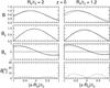 |
Fig. 3 Profiles of the magnetic field magnitude B, magnetic field components By and Bz, and the δ angle along the x axis for a toroidal flux rope with the Tsuji (solid lines), Miller & Turner (dashed lines), and modified Miller & Turner (dotted lines) solutions (α> 0). The Bx component is zero for all solutions, therefore, it is not shown. Magnetic field is scaled by maximum value inside the respective flux rope. The δ angle, the angle between B and rot B, indicates how the force-free condition is fulfilled; this angle is zero for the Tsuji solution. Two columns are plotted for two aspect ratios, 2 (left) and 1.2 (right). |
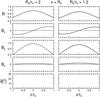 |
Fig. 4 Profiles of quantities along a line parallel to the z axis and crossing the toroid’s circular axis for a toroidal flux rope with the Tsuji (solid lines), Miller & Turner (dashed lines), and modified Miller & Turner (dotted lines) solutions (α> 0). Format is similar to Fig. 3. The δ angle is zero for the Tsuji and Miller & Turner solutions. Two columns are plotted for two aspect ratios, 2 (left) and 1.2 (right). |
Figure 5 displays magnetic field magnitude distributions at circular cross sections of toroidal flux ropes for all three compared fields and two aspect ratios. In addition, in all cross sections there are six closed lines showing magnetic surfaces on which helical magnetic field lines lie. The first lines, the smallest ones and similar to small open circles, indicate positions of magnetic axes. The largest magnetic surfaces are circular and give the flux rope boundary. There are two symbols in each cross section. The “+” symbol indicates the geometric center of the cross section (the circle) and has coordinates [0, 0] in the plot. Here the toroid’s circular axis crosses the xz plane. The bullet determines the place of the maximum field magnitude (Bmax). We see that positions of the magnetic axes are shifted to the right from the geometric center, away from the toroid’s hole (cf. with Figs. 3 and 4 in Tsuji 1991), while positions of Bmax are shifted to the left, toward the toroid’s hole, and these shifts increase with decreasing aspect ratio. Their positions, and also the shapes of magnetic surfaces in the case of the modified Miller & Turner solution, are more similar to the Tsuji solutions than it is in the case of the Miller & Turner solution, even for low aspect ratios. However, there is a significant qualitative difference. Magnetic magnitude contours are prolate in the Tsuji field, while they are oblate in the Miller & Turner field and its modification, and this difference is more pronounced in the former field.
 |
Fig. 5 Magnetic field magnitude distribution inside toroidal flux ropes (their circular cross sections) with the Tsuji (T), Miller & Turner (MT), and modified Miller & Turner (mMT) solutions (magnitude is scaled by the maximum value Bmax inside a corresponding rope; the position of Bmax shows the bullet). The ovals are magnetic surfaces (more precisely, their xz cross sections) and the symbols “+” indicate geometric centers of the ropes. Two columns are plotted for two aspect ratios, 2 (left) and 1.2 (right). |
Figure 6 is in the same format as Fig. 5, except the magnetic field magnitude is replaced by the δ angle and the Tsuji solution is missing because it has δ = 0 identically. The Miller & Turner solution fulfills the force-free condition reasonably well, while the modified Miller & Turner solution has large deviations near the boundary, e.g. δ is over 60° in a small region adjacent to the toroid’s hole for the 1.2 aspect ratio case (near the point [−1, 0] in the figure). Figure 7 shows the δ angle averaged over the toroid’s volume as a function of the aspect ratio for both solutions, which confirms the fact that the Miller & Turner solution fulfills the force-free condition better.
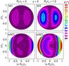 |
Fig. 6 Distribution of the δ angle inside toroidal flux ropes (their circular cross sections) with the Miller & Turner (MT) and modified Miller & Turner (mMT) solutions for two aspect ratios, 2 (left column), and 1.2 (right column). |
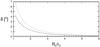 |
Fig. 7 The δ angle averaged over the toroid’s volume for flux ropes with the Miller & Turner (dashed line) and modified Miller & Turner (dotted line) solutions as a function of aspect ratio R0/r0. |
Now we shall compare helicity of our toroidal flux ropes. In Fig. 8 a unitless quantity h is plotted as a function of the aspect ratio for all three compared fields; h is derived from the helicity as  (41)where V is the volume of the toroidal flux rope, and
  , Bmax is the maximum field magnitude inside it. For example, for the Miller & Turner solution it is
 ![Mathematical equation: \begin{equation} \label{h1} h^\mathrm{(MT)} = \left(\frac{B_0}{B_\mathrm{max}}\right)^2 \left[2-\frac{1}{4} \left(1+ \frac{1}{a_0^2}\right)\left(\frac{r_0}{R_0}\right)^2\right] {J}_1^2(a_0), \end{equation}](/articles/aa/full_html/2015/08/aa26242-15/aa26242-15-eq121.png) (42)in the limit of large aspect ratios, we get
(42)in the limit of large aspect ratios, we get  (43)This quantity is also h of the toroidally adjusted Lundquist solution and represents an asymptotic value of the other solutions for large aspect ratios (see the dashed-dotted line in Fig. 8). Comparing curves for three fields, we see that the formula (37) for the helicity derived from the Miller & Turner solution approximates the correct dependence resulting from the Tsuji solution quite well, even for very low aspect ratios where the modified Miller & Turner solution fails.
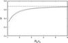 |
Fig. 8 Unitless quantity h derived from the magnetic helicity (see text for the definition) as a function of the aspect ratio R0/r0 for toroidal flux ropes with the Tsuji (solid line), Miller & Turner (dashed line), and modified Miller & Turner (dotted line) solutions. The horizontal dashed-dotted line shows an asymptotic value to which all solutions tend for large aspect ratios. |
4. Conclusions
Approximate constant-alpha force-free solutions in an ideal toroid, namely the toroidally adjusted Lundquist solution (Marubashi 1997), Miller & Turner (1981) solution, and modified Miller & Turner solution (Romashets & Vandas 2003b), were compared with the exact solution (Tsuji 1991). The modified Miller & Turner solution is exactly solenoidal for all aspect ratios, while the remaining two are only approximately solenoidal. For large aspect ratios (>10), all solutions practically coincide. Comparing the magnetic field distribution at the flux-rope cross section, the field maximum is shifted toward the toroid’s hole and the shift increases with the aspect ratio decrease. For low aspect ratios (<3), the position of Bmax is better matched by the modified Miller & Turner than the Miller & Turner field. The toroidally adjusted Lundquist field does not adequately describe the field distribution for smaller aspect ratios because it is always symmetric around the center of the cross section (with Bmax at the center). The position of the magnetic axis is shifted in opposite direction and is satisfactorily matched by both the Miller & Turner field and its modification. These two fields fulfill the force-free condition only approximately and, for small aspect ratios, the Miller & Turner solution satisfies it much better. A simple formula for magnetic helicity was derived for the Miller & Turner field and its comparison with the accurate magnetic helicity calculated numerically from the Tsuji solution shows a reasonably good agreement even for very low (<2) aspect ratios (contrary to the helicity derived from the modified Miller & Turner solution, which significantly differs for them). One can conclude that the Miller & Turner solution is a reasonable substitute for the exact solution even for low aspect ratios (≈2). In magnetic cloud research, when there is a need to approximate magnetic cloud locally by a constant-alpha force-free toroid, the Miller & Turner solution is a suitable magnetic field configuration for all aspect ratios met in practice.
Acknowledgments
This work was supported by project 14-19376S from GA ČR and by the AV ČR grant RVO:67985815.
References
- Burlaga, L. F. 1988, JGR, 93, 7217 [Google Scholar]
- Burlaga, L. F., & Behannon, K. W. 1982, Sol. Phys., 81, 181 [NASA ADS] [CrossRef] [Google Scholar]
- Burlaga, L., Sittler, E., Mariani, F., & Schwenn, R. 1981, JGR, 86, 6673 [Google Scholar]
- Burlaga, L. F., Klein, L. W., Sheeley, Jr., N. R., et al. 1982, GRL, 9, 1317 [Google Scholar]
- Burlaga, L. F., Lepping, R. P., & Jones, J. A. 1990, in Physics of Magnetic Flux Ropes, Geophys. Monogr. Ser., 58, eds. C. T. Russell, E. R. Priest, & L. C. Lee (Washington, D.C.: AGU), 373 [Google Scholar]
- Cartwright, M. L., & Moldwin, M. B. 2010, JGR, 115, A08102 [NASA ADS] [Google Scholar]
- Chen, J., & Garren, D. A. 1993, GRL, 20, 2319 [Google Scholar]
- Dasso, S., Mandrini, C. H., Démoulin, P., & Farrugia, C. J. 2003, JGR, 108, 8037 [Google Scholar]
- Hidalgo, M. A. 2013, ApJ, 766, 125 [NASA ADS] [CrossRef] [Google Scholar]
- Hidalgo, M. A. 2014, ApJ, 784, 67 [NASA ADS] [CrossRef] [Google Scholar]
- Ivanov, K. G., Harshiladze, A. F., Eroshenko, E. G., & Styazhkin, V. A. 1989, Sol. Phys., 120, 407 [NASA ADS] [CrossRef] [Google Scholar]
- Janvier, M., Demoulin, P., & Dasso, S. 2013, A&A, 556, A50 [NASA ADS] [CrossRef] [EDP Sciences] [Google Scholar]
- Klein, L. W., & Burlaga, L. F. 1982, JGR, 87, 613 [Google Scholar]
- Krimigis, S., Sarris, E., & Armstrong, T. 1976, Trans. AGU, 57, 304 [Google Scholar]
- Lepping, R. P., Jones, J. A., & Burlaga, L. F. 1990, JGR, 95, 11957 [NASA ADS] [CrossRef] [Google Scholar]
- Lepping, R. P., Berdichevsky, D. B., Wu, C.-C., et al. 2006, Ann. Geophys., 24, 215 [NASA ADS] [CrossRef] [Google Scholar]
- Lepping, R. P., Wu, C.-C., & Berdichevsky, D. B. 2015, Sol. Phys., 290, 553 [NASA ADS] [CrossRef] [Google Scholar]
- Lundquist, S. 1950, Ark. Fys., 2, 361 [Google Scholar]
- Mandrini, C. H., Pohjolainen, S., Dasso, S., et al. 2005, A&A, 434, 725 [NASA ADS] [CrossRef] [EDP Sciences] [Google Scholar]
- Marubashi, K. 1997, in Coronal Mass Ejections, Geophys. Monogr. Ser., 99, eds. N. Crooker, J. Joselyn, & J. Feyman (Washington, D.C.: AGU), 147 [Google Scholar]
- Marubashi, K., & Lepping, R. P. 2007, Ann. Geophys., 25, 2453 [NASA ADS] [CrossRef] [Google Scholar]
- Miller, G., & Turner, L. 1981, Phys. Fluids, 24, 363 [NASA ADS] [CrossRef] [Google Scholar]
- Moldwin, M. B., Ford, S., Lepping, R., Slavin, J., & Szabo, A. 2000, GRL, 27, 57 [Google Scholar]
- Press, V. H., Teukolsky, S. A., Vetterling, W. T., & Flannery, B. P. 2002, Numerical Recipes in C, The Art of Scientific Computing, Second Edition (New York: Cambridge University Press) [Google Scholar]
- Romashets, E. P., & Vandas, M. 2003a, GRL, 30, 2065 [NASA ADS] [CrossRef] [Google Scholar]
- Romashets, E. P., & Vandas, M. 2003b, in Proc. ISCS 2003 Symp., Solar Variability as an Input to the Earth’s Environment, ed. A. Wilson (Noordwijk: ESTEC), ESA SP, 535, 535 [NASA ADS] [Google Scholar]
- Shimazu, H., & Marubashi, K. 2000, JGR, 105, 2365 [Google Scholar]
- Tsuji, Y. 1991, Phys. Fluids B, 3, 3379 [NASA ADS] [CrossRef] [Google Scholar]
- Vandas, M., & Romashets, E. P. 2010, in Twelve International Solar Wind Conf., eds. M. Maksimovic, K. Issautier, N. Meyer-Vernet, M. Moncuquet, & F. Pantellini (Melville, New York: AIP), AIP Conf. Proc., 1216, 403 [Google Scholar]
- Vandas, M., Odstrcil, D., & Watari, S. 2002, JGR, 107, 2156 [Google Scholar]
Appendix A: Coefficients of the Tsuji solution
The coefficients  are defined by
 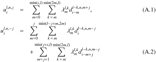 and valid for j ≥ 0. The coefficients
  are given by
 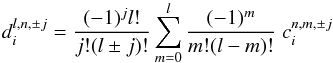 (A.3)where
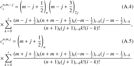 The expression (c)n is the Pochhammer symbol or rising factorial, defined as (c)n = c(c + 1)...(c + n − 1) with (c)0 = 1. The coefficients
  are defined for l ≥ 0, 0 ≤ m ≤ l, and m ≤ n ≤ min(2m,l) by
 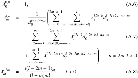 It is assumed in summations that when the upper limit is lower than the lower limit, the summation is not performed.
It holds for all l ≥ 0, i ≥ 0, n ≥ 0, j ≥ 0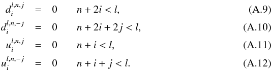 The coefficients do not depend on toroid’s parameters; they can be pre-calculated. For numerical calculations, the unlimited sums are cut at some number, and we used 20. This number depends on value of aspect ratio that is to be reached: the lower aspect ratio is, the higher the number must be. Because the coefficients are defined recursively, for given l, calculations are performed in increasing order of m and then decreasing order of n. Here are some values to check implementation (all are exact numbers):
  ,
,  ,
,  ,
,  ,
,  ,
,  ,
,  ,
,  ,
,  ,
,  ,
,  ,
, 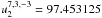 . Some additional values of are listed in Table 1 of Tsuji (1991).
All Tables
All Figures
|
Fig. 1 Two coordinate systems shown separately in a) and b), that we used for descriptions of toroidal magnetic field configurations. Cross sections of our toroid’s surface (with major and minor radii, R0 and r0, respectively) with the xz plane are shown with the thick circles. Our toroid has a circular axis at |
| In the text | |
|
Fig. 2 Dependence of the force-free constant α on the aspect ratio R0/r0 of a toroid. For large aspect ratios, it tends to an asymptotic value, shown with the dashed-dotted line, which is consistent with the Lundquist solution. It is the first root of the Bessel function J0, a0. |
| In the text | |
|
Fig. 3 Profiles of the magnetic field magnitude B, magnetic field components By and Bz, and the δ angle along the x axis for a toroidal flux rope with the Tsuji (solid lines), Miller & Turner (dashed lines), and modified Miller & Turner (dotted lines) solutions (α> 0). The Bx component is zero for all solutions, therefore, it is not shown. Magnetic field is scaled by maximum value inside the respective flux rope. The δ angle, the angle between B and rot B, indicates how the force-free condition is fulfilled; this angle is zero for the Tsuji solution. Two columns are plotted for two aspect ratios, 2 (left) and 1.2 (right). |
| In the text | |
|
Fig. 4 Profiles of quantities along a line parallel to the z axis and crossing the toroid’s circular axis for a toroidal flux rope with the Tsuji (solid lines), Miller & Turner (dashed lines), and modified Miller & Turner (dotted lines) solutions (α> 0). Format is similar to Fig. 3. The δ angle is zero for the Tsuji and Miller & Turner solutions. Two columns are plotted for two aspect ratios, 2 (left) and 1.2 (right). |
| In the text | |
|
Fig. 5 Magnetic field magnitude distribution inside toroidal flux ropes (their circular cross sections) with the Tsuji (T), Miller & Turner (MT), and modified Miller & Turner (mMT) solutions (magnitude is scaled by the maximum value Bmax inside a corresponding rope; the position of Bmax shows the bullet). The ovals are magnetic surfaces (more precisely, their xz cross sections) and the symbols “+” indicate geometric centers of the ropes. Two columns are plotted for two aspect ratios, 2 (left) and 1.2 (right). |
| In the text | |
|
Fig. 6 Distribution of the δ angle inside toroidal flux ropes (their circular cross sections) with the Miller & Turner (MT) and modified Miller & Turner (mMT) solutions for two aspect ratios, 2 (left column), and 1.2 (right column). |
| In the text | |
|
Fig. 7 The δ angle averaged over the toroid’s volume for flux ropes with the Miller & Turner (dashed line) and modified Miller & Turner (dotted line) solutions as a function of aspect ratio R0/r0. |
| In the text | |
|
Fig. 8 Unitless quantity h derived from the magnetic helicity (see text for the definition) as a function of the aspect ratio R0/r0 for toroidal flux ropes with the Tsuji (solid line), Miller & Turner (dashed line), and modified Miller & Turner (dotted line) solutions. The horizontal dashed-dotted line shows an asymptotic value to which all solutions tend for large aspect ratios. |
| In the text | |
Current usage metrics show cumulative count of Article Views (full-text article views including HTML views, PDF and ePub downloads, according to the available data) and Abstracts Views on Vision4Press platform.
Data correspond to usage on the plateform after 2015. The current usage metrics is available 48-96 hours after online publication and is updated daily on week days.
Initial download of the metrics may take a while.