| Issue |
A&A
Volume 580, August 2015
|
|
|---|---|---|
| Article Number | A31 | |
| Number of page(s) | 10 | |
| Section | Planets and planetary systems | |
| DOI | https://doi.org/10.1051/0004-6361/201425519 | |
| Published online | 23 July 2015 | |
Long-lived, long-period radial velocity variations in Aldebaran: A planetary companion and stellar activity⋆,⋆⋆
1 Thüringer Landessternwarte Tautenburg, Sternwarte 5, 07778 Tautenburg, Germany
e-mail: artie@tls-tautenburg.de
2 McDonald Observatory, The University of Texas at Austin, Austin, TX 78712, USA
3 Institut für Astrophysik, Georg-August-Universität, Friedrich-Hund-Platz 1, 37077 Göttingen, Germany
4 Korea Astronomy and Space Science Institute, 776, Daedeokdae-Ro, Youseong-Gu, Daejeon 305-348, Korea
5 1234 Hewlett Place, Victoria, BC, V8S 4P7, Canada
6 Department of Physics and Astronomy, University of Victoria, Victoria, BC, V8W 3P6, Canada
7 Astronomy Department, Box 351580, University of Washington, Seattle, WA 98195-1580, UK
8 National Astronomical Research Institute of Thailand, 191 Siriphanich Bldg., Huay Kaew Rd., Suthep, Muang, 50200 Chiang Mai, Thailand
9 Crimean Astrophysical Observatory, Nauchny, Crimea, 98409, Ukraine
10 Physikalisches Institut, Center for Space and Habitability, University of Bern, Sidlerstrasse 5, 3012 Bern, Swithzerland
11 Konkoly Observatory, Research Centre for Astronomy and Earth Sciences, Hungarian Academy of Sciences, 1121 Budapest, Konkoly Thege. Miklós. út 15-17, Hungary
12 INAF-Osservatorio Astronomico di Padova, vicolo dell’O servatorio 5, 35122 Padova, Italy
Received: 15 December 2014
Accepted: 29 April 2015
Aims. We investigate the nature of the long-period radial velocity variations in α Tau first reported over 20 yr ago.
Methods. We analyzed precise stellar radial velocity measurements for α Tau spanning over 30 yr. An examination of the Hα and Ca II λ8662 spectral lines, and Hipparcos photometry was also done to help discern the nature of the long-period radial velocity variations.
Results. Our radial velocity data show that the long-period, low amplitude radial velocity variations are long-lived and coherent. Furthermore, Hα equivalent width measurements and Hipparcos photometry show no significant variations with this period. Another investigation of this star established that there was no variability in the spectral line shapes with the radial velocity period. An orbital solution results in a period of P = 628.96 ± 0.90 d, eccentricity, e = 0.10 ± 0.05, and a radial velocity amplitude, K = 142.1 ± 7.2 m s-1. Evolutionary tracks yield a stellar mass of 1.13 ± 0.11 M⊙, which corresponds to a minimum companion mass of 6.47 ± 0.53 MJup with an orbital semi-major axis of a = 1.46 ± 0.27 AU. After removing the orbital motion of the companion, an additional period of ≈520 d is found in the radial velocity data, but only in some time spans. A similar period is found in the variations in the equivalent width of Hα and Ca II. Variations at one-third of this period are also found in the spectral line bisector measurements. The ~520 d period is interpreted as the rotation modulation by stellar surface structure. Its presence, however, may not be long-lived, and it only appears in epochs of the radial velocity data separated by ~10 yr. This might be due to an activity cycle.
Conclusions. The data presented here provide further evidence of a planetary companion to α Tau, as well as activity-related radial velocity variations.
Key words: stars: individual: αTu / techniques: radial velocities
Based in part on observations obtained at the 2-m-Alfred Jensch Telescope at the Thüringer Landessternwarte Tautenburg and the telescope facilities of McDonald Observatory.
Tables 3−9 are only available at the CDS via anonymous ftp to cdsarc.u-strasbg.fr (130.79.128.5) or via http://cdsarc.u-strasbg.fr/viz-bin/qcat?J/A+A/580/A31
© ESO, 2015
1. Introduction
Low amplitude radial velocity (RV) variations with a period of 645 days were first reported in the K giant star α Tau (=Aldebaran = HR 1457 = HD 29139 = HIP 21421) by Hatzes & Cochran 1993 (hereafter HC93). HC93 hypothesized that one cause for these variations was a planetary companion with m sin i = 11.4 MJup, when assuming a stellar mass of 2.5 M⊙. There was some hint that these RV variations were long-lived because measurements taken almost a decade earlier by Walker et al. (1989) were consistent in amplitude and phase with the measurements of HC93. A subsequent analysis of the spectral line shapes (line bisectors) by Hatzes & Cochran (1998) showed no evidence of variations with the 645 d RV period, although they did find evidence of a 50 d period in the line bisectors that they attributed to stellar oscillations. This seemed to provide further support for the presence of a planetary companion. However, the confirmation of such a hypothesis was still in doubt owing to the unknown intrinsic variability of K giant stars.
Subsequent to the discovery of RV variations in Aldebaran it has been well established that K giant stars can indeed possess giant extrasolar planets (e.g., Frink et al. 2002; Setiawan et al. 2003; Hatzes et al. 2005; Döllinger et al. 2007; Niedzielski et al. 2009). In particular, the long period RV variations for one of the K giants studied by HC93, β Gem, were recently confirmed to be caused by a giant planet with a mass of 2.3 MJup (Hatzes et al. 2006). This was established by long-lived, coherent RV variations spanning 25 yr, along with the lack of variations in the spectral line shapes and Ca II emission. Reffert et al. (2006) and Han et al. (2008) also confirmed the long-lived nature of the RV variations of β Gem. RV variations caused by a substellar companion should not show any variations in the spectral lines with the same period as the planet. In the case of α Tau, this has already been established by the line bisector measurements of Hatzes & Cochran (1998). Long-lived RV variations lasting several decades would provide additional compelling evidence for the planet hypothesis, as was the case for β Gem. For α Tau this is problematical as this star can show intrinsic variations of ≈100 m s-1. A large number of measurements over a long time base are needed to extract the long period RV signal with confidence.
Here, we present additional measurements of α Tau taken with the coude échelle spectrograph of the Thüringer Landessternwarte Tautenburg (TLS), the Tull Spectrograph of the McDonald 2.7 m telescope, and the Bohyunsan Observatory Échelle Spectrograph (BOES) spectrograph of the Bohyunsan Optical Astronomy Observatory (BOAO). These measurements are combined with previous measurements to produce a total baseline of over 30 yr. The combined data clearly show that a period near 629 d has been present with the same amplitude and phase for the entire time span lending further evidence to the planet hypothesis for the long period RV variations of α Tau. These data also show additional variations which are most likely due to rotational modulation by surface features.
2. Stellar parameters
The K5 III star α Tau is at a distance of 20.43 ± 0.32 pc as measured by Hipparcos (van Leeuwen 2007). Richichi & Roccatagliata (2005) presented a few very accurate radius measurements of α Tau. They determined a limb-darkened angular diameter of 20.058 ± 0.03 mas and a uniform disk angular diameter of 19.96 ± 0.03 mas yielding a radius of 45.1 ± 0.1 R⊙ for the limb-darkened case. By virtue of its large angular diameter and location in the ecliptic there have been a large number of angular diameter measurements for α Tau using interferometry or lunar occultations. Richichi & Roccatagliata (2005) discussed these in detail and noted that there was considerable scatter in these measurements corresponding to R = 36−46 R⊙ at 550 nm that was larger than the formal errors. The source of such discrepancies is not known.
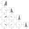 |
Fig. 1 Probability density functions (PDF) for various parameters of α Tau. The histogram (on right) for each row shows the PDF for (top to bottom) stellar age, mass, radius, and surface gravity. The correlation plots on each row show how that parameter correlates with the other parameters. |
McWilliam (1990) measured an effective temperature of 3910 K, a metalicity of [Fe/H] = −0.34 ± 0.21, and a surface gravity, log g = 1.59 ± 0.27. We also derived the stellar parameters for α Tau using a high signal-to-noise spectrum taken with the coude échelle spectrograph of the TLS. The details of the analysis method will be given in a forthcoming paper. Briefly, we used the model atmospheres of Gustafsson et al. (1975) and plane-parallel geometry along with the assumption of local thermodynamic equilibrium. The iron content was determined from the equivalent width of over one hundred Fe I lines and eight Fe II lines.
The effective temperature was determined by imposing that the Fe I abundance does not depend on the excitation potential of the lines. The surface gravity was determined using the Fe I and Fe II ionization equilibrium.
Our analysis yielded Teff = 4055 ± 70 K, log g = 1.20 ± 0.1, and [Fe/H] = −0.27 ± 0.05. Our abundance and log g values are consistent with the McWilliam (1990) analysis and the value determined from the evolutionary tracks (Fig. 1). The determination of Teff is also in line with literature values from the past 20 yr. These range as low as 3875 K (Luck & Challener 1995) and as high as 4131 K (Kovacs 1983).
The basic stellar parameters such as mass, radius, and age were determined using theoretical isochrones and a modified version of Jorgensen & Lindegren’s (2005) method also described in da Silva et al. (2006). Figure 1 shows the probability density functions (PDF) of the derived parameters. The PDF for the age appears truncated because the prior includes a maximum age for the star. The PDF mean values and the 68% confidence level for the stellar age and mass are listed in Table 1. The first figures of each row also show how the current parameter (row) correlates with the previous (rows from above) parameters. For instance, a radius ~5% larger than the one estimated would imply a smaller log g by ~0.02 dex, a decrease of ~4% in mass, and an increase of ~28% in age.
Stellar parameters of α Tau.
The radius determined by this method, R = 36.68 ± 2.46 R⊙, is less than the Richichi & Roccatagliata (2005) nominal value. However, it is still within the range of radius measurements that have been made for this star. In Table 1 we list the interferometric value of the radius as determined by Richichi & Roccatagliata (2005). The stellar mass derived by this method is 1.13 ± 0.11 M⊙ which we adopt for the subsequent analysis. We note that the surface gravity determined via our spectral analysis is consistent with the mass and radius for the star listed in Table 1. Assuming that α Tau did not lose significant mass loss as it evolved to its present state, then its progenitor star on the main sequence would have had a spectral type of ~F7.
3. The radial velocity data
Seven independent data sets of high precision radial velocity data were used for our analysis. Precise RV measurements were also made with a hydrogen–fluoride (H–F) cell as part of the CFHT survey (hereafter the “CFHT” data set) of Walker et al. (1989) as well as additional measurements from the Dominion Astrophysical Observatory (hereafter “DAO” data set) using the same technique. See Campbell & Walker (1979) and Larson et al. (1993b) for a description of the H-F measurements. For the remaining five RV data sets an iodine (I2) cell provided the wavelength reference. These include the original measurements using the McDonald Observatory 2.1 m telescope (hereafter “McD-2.1 m” data set) and the coude spectrograph in the so-called “cs11” focus (hereafter “McD-CS11” data set) of the 2.7 m telescope at McDonald Observatory. We should note that the we did not include the McDonald data that were used for the bisector measurements of Hatzes & Cochran (1998). These were taken using telluric lines as a wavelength reference which had a lower precision than the iodine wavelength calibration or H–F methods.
The latest McDonald measurements were taken using the Tull Spectrograph at the so-called “cs23” focus (hereafter the “McD-Tull” data set) as part of a long-term planet search program (e.g. Cochran et al. 1997; Endl et al. 2004; Robertson et al. 2012).
Observations of α Tau were made as part of the planet search program of the Thüringer Landessternwarte Tautenburg (“TLS” data set) and at the Bohyunsan Optical Astronomy Observatory. The TLS program uses the high resolution coude échelle spectrometer of the Alfred Jensch 2 m telescope and an iodine absorption cell placedbefore the entrance slit of the spectrograph. The instrument is a grism crossed-dispersed échelle spectrometer that has a resolving power R (λ/Δλ) = 67 000 and wavelength coverage 4630−7370 Å when using the so-called “Visual” grism. A more detailed description of radial velocity measurements from the TLS program can be found in Hatzes et al. (2005).
The BOAO measurements (“BOAO” data set) were made with the fiber-fed Bohyunsan Observatory Échelle Spectrograph (BOES). BOES has a wavelength coverage of 3600−10 500 Å. The resolving power for the observations was 90 000. An iodine absorption cell was also used to provide the wavelength reference for the precise RV measurements. See Kim et al. (2006) for a more detailed description of the instrument and data analysis used for these RV measurements.
Table 2 lists the journal of observations which includes the data set, time coverage, the wavelength reference employed, the number of observations, and the root mean square scatter (rms) about the orbital solution presented in Sect. 4.
Tables 3–9 list the RV measurements from the seven data sets. Each instrument only measures a relative RV, thus each data set has a different zero-point offset. In Sect. 4 the relative zero-point offsets were calculated as part of the global fit to the orbital solution. These offsets have been applied in the tabulated data and the displayed measurements. α Tau is a bright star and typically multiple measurements were made each night. Nightly averages were used in the analysis and the plots and are listed in the tables.
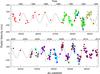 |
Fig. 2 Radial velocity measurements for α Tau from the seven data sets: CFHT (diamonds), DAO (inverted triangles), McD-2.1 m (circles), McD-CS11 (squares), McD-Tull (sideways triangles), TLS (triangles), and BOAO (pentagons). Zero point corrections have been applied to the individual data sets before plotting (see text). The curve represents the orbital solution (see Table 10). The vertical dash represents the peak-to-peak variations of the stellar oscillations. |
Data sets used in the orbital solution.
The RV measurements for all data sets (with the appropriate offsets applied, see below) are shown in Fig. 2. There appears to be long-lived sinusoidal variations that span the entire data sets and have a scatter of ≈100 m s-1.
The bottom panel of Fig. 3 shows the Lomb-Scargle (L-S) periodogram (Lomb 1976; Scargle 1982) of all the RV measurements with the proper zero point offsets as found in the orbit fitting subtracted from each data set (see below). Although each data set has a different precision, the intrinsic RV jitter of the star is many factors larger than these and is approximately the same for all data sets. It is therefore not important to weight the periodogram by the different errors. There is a highly significant peak at a period, P ≈ 630 d. The false alarm probability (FAP) of this signal using the equation in Scargle (1982) is FAP ≈ 10-20. This signal appears to be long-lived as it appears in the RV measurements taken prior to 2000 (JD < 2 450 000, top panel), and after 2000 (middle panel).
4. Orbital solutions
An orbital solution was calculated using the combined data sets and the program Gaussfit (Jefferys et al. 1988). The velocity zero point for each data set was allowed to be a free parameter. These individual zero points in the velocity were subtracted from each data set before plotting in Fig. 2. (Tables 3–9 list the zero-point subtracted data.)
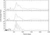 |
Fig. 3 L-S periodogram of the RV measurements taken prior to JD = 2 450 000 (top), after JD = 2 450 000 (middle), and the full data set (bottom). |
Our initial solution resulted in a period of P = 628.07 ± 0.82 d, eccentricity, e = 0.15 ± 0.04 and a velocity amplitude, K = 158.0 ± 6.5 m s-1. The referee noted that some of the data sets (TLS and McD-Tull) had many measurements that were clumped in some epochs. This was particularly true for the TLS data as numerous RV measurements were taken over several consecutive nights in order to study the stellar oscillations. The referee expressed a valid concern that this “clumping” may have given a higher weight when computing the orbit. This could have a strong effect primarily on the orbital eccentricity and velocity amplitude.
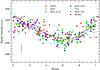 |
Fig. 4 Radial velocity measurements for α Tau from the seven data sets phased to the orbital period.For the TLS and McD-Tull data we plot run-binned averages that were used in the orbital solution. The solid line is the orbital solution and the vertical line the peak-peak short term intrinsic RV variations observed for this star. Symbols are the same as for Fig. 2. Error bars for individual measurements are not shown for clarity and because the scatter is dominated by the intrinsic stellar variability. |
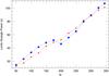 |
Fig. 5 L-S power (z) of the 629 d period as a function of the number of data points used in the periodogram calculation (circles). The power, z, as a function of the number of data points for simulated data (triangles). |
Therefore, we binned the RV values over individual observing runs for the TLS and McD-Tull data. This resulted in an average RV value over typically three to five nights. The orbital parameters using all the data, but the run-binned values from TLS and McD-Tull, are listed in Table 10. These include the orbital period, P, the time of periastron, the radial velocity (K) amplitude, the eccentricity, e, the argument of periastron, ω, the mass function (f(m)), the minimum companion mass, m sin i, and the orbital semi-major axis, a. Note that using the run-binned averages only results in a slight and insignificant decrease in the eccentricity and K-amplitude. Figure 4 shows the RV measurements phase-folded and the orbital solution.
Orbital parameters for the companion to α Tau.
The rms scatter about the orbital solution from the individual data sets is listed in Table 2 and is about ≈100 m s-1 for each set. This is mostly due to intrinsic variability from stellar oscillations. Alpha Tau shows RV variations of several hundred m s-1 peak-to-peak in the course of several nights. For example, the RV of α Tau changed by ≈220 m s-1 between JD = 2 454 071 and 2 454 076. This time scale and amplitude are typical for oscillations in more evolved K giants (e.g. Hatzes & Cochran 1994). Therefore, we take ≈±100 m s-1 as the intrinsic RV “jitter” of the star and as our “working” precision. This is shown by the vertical lines in Figs. 2 and 4.
5. The nature of the RV variations
The fact that the RV variations seem to be long-lived and coherent for over 30 years strongly argues that they are indeed due to a sub-stellar companion. However, because α Tau is an evolved giant star it is prudent to examine whether the RV period is present in other measured quantities. As noted earlier, Hatzes & Cochran (1998) already established that there were no spectral line shape variations with a period of ≈645 d based on very high resolution (R = 220 000) spectral data. The spectral line shape measurements thus do not support rotational modulation as a cause for the 629 d period RV variations. Additional evidence can be found by examining the photometry and activity indicators as well as the stability of the RV period.
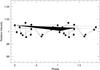 |
Fig. 6 Hipparcos photometry phased to the 629 d orbital period. |
5.1. Stability of the RV variations
Although the orbital solution fits most of the RV data very well, there are times when the measurements deviate from this solution. In particular, the McD-Tull data near JD = 2 452 600 (2002−2003) show a rapid increase in the RV, but at a later phase to the orbital solution. Also, both the McD-Tull and TLS data at JD = 2 453 000 (2003−2004) show considerable scatter that is not centered on the orbital solution.
One property of long-lived, coherent periodic signals is that the L-S power, and thus statistical significance, should increase with the number of data points. The circles in Fig. 5 show the growth of the L-S power as a function of the number of data points taken in chronological order. The temporary decrease in power at N ≈ 200 is related to the discrepant RV data in the years 2002 to early 2004.
Triangles represent results from a simulation where the orbital solution was sampled in the same manner as the data and with random noise at a level of 100 m s-1 added. The slope of the power increase for the real data is consistent with that of a long-lived, coherent signal.
5.2. Hipparcos photometry
The Hipparcos photometry for α Tau covers the time interval from 1990.1 to 1992.6 and is therefore contemporaneous with a part of the RV measurements. Figure 6 shows this photometry phased to the 629 d orbital period. Although there is considerable scatter in the data there are no obvious sinusoidal variations. Observations of α Tau made with the MOST space telescope reveal periodic photometric variations with a peak-to-peak value of ≈ 0.02 mag (Matthews, priv. comm.) which is comparable to the scatter in the Hipparcos photometry.
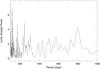 |
Fig. 7 L-S periodogram of the ΔEW8662 variations. |
5.3. Variations in activity indicators
One explanation for the 629 d period in α Tau is that it is due to rotational modulation caused by surface structure. Even though this is not supported by the previous bisector measurements, it is still worth investigating other activity indicators. Unfortunately, only the McD-Tull observations cover the Ca II H & K lines. For the CFHT and DAO observations we must use the Ca II 8662 Å line and Hα for the TLS data as activity diagnostics.
5.3.1. Ca II 8662 Å variations
Larson et al. (1993a) showed that the Ca II λ8662 line is suitable for measuring chromospheric activity. Figure 7 shows the L-S periodogram of the variations in Ca II λ8662 equivalent width, ΔEW8662, measured from the CFHT and DAO data. There is no significant power at the orbital, or any other period.
5.3.2. Ca II variations
The McDonald Ca II S-index measurements from the McD-Tull data set show long term variations with a possible period of P ≈ 4000 d (Fig. 8). The FAP for this signal is FAP ≈ 0.08 as determined from a bootstrap analysis (Murdoch et al. 1993; Kürster et al. 1997). A sine fit to these data results in P = 4320 ± 450 d. This periodic signal is only suggestive as there are insufficient data with too much scatter to be convincing. However, the rough time scales of this possible periodic variations is consistent with long term variations in the RV residuals (see below). After removing this long-term trend the L-S periodogram shows power at a period, P = 521 ± 10 d (top panel of Fig. 9). This peak is not significant with FAP ≈ 0.2, but as we shall see it is close to a value found in the residual RV and Hα measurements.
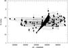 |
Fig. 8 Variations of the McDonald S-index measurements with time. The line represents a sine fit with a period P = 4320 ± 450 d. |
5.3.3. Hα variations
The TLS spectral data cover the Balmer Hα line which is also useful for discerning whether RV variability is due to intrinsic stellar variability from activity (see Kürster et al. 2003). Thus we measured the equivalent width of Hα from the TLS spectra focusing on the time span JD = 2 452 656−2 454 160 in order to investigate the cause for the large scatter in the residuals.For main sequence stars such a measurement is problematic because of blending of the stellar Hα with telluric lines. However, in a giant star like Aldebaran this is much easier because the Hα line is so narrow. We could thus use a window of only ±1.0 Å centered on Hα to measure the equivalent width using a Gaussian fit to the profile. The two prominent H2O absorption lines at 6560.5 Å and 6565.5 Å, which have equivalent widths of 22 mÅ and 14 mÅ, respectively, are outside of the measurement window.
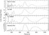 |
Fig. 9 Top to bottom: L-S periodograms of the McDonald S-index, Hα equivalent width, Hα FWHM, and residual RV measurements. The RV residuals were taken from the time interval 2004.7−2008.2 (see text). |
The middle-upper panel of Fig. 9 shows the L-S periodogram of the Hα equivalent width variations. There are two significant peaks, one corresponding to a period of 892 d and another corresponding to a period of 520 d. These periods are clearly aliases of each other as fitting the data with the sine function of one period and removing it from the data causes the other to disappear. The FAP estimated using a bootstrap of 2 × 10⁵ random shuffles of the RV data yielded no instance when the random periodogram had more L-S than the data. The FAP is thus less than 5 × 10⁻⁵.
We also measured the full width at half maximum (FWHM) of the Hα line. The FWHM of photospheric lines have been shown to be good tracers of variations due to activity in active main sequence stars (Queloz et al. 2009). The FWHM of Hα may also provide a tracer of chromospheric activity. Furthermore, the FWHM may be less sensitive to contamination by telluric lines as would be the case for equivalent width measurements. The lower-middle panel of Fig. 9 is the L-S periodogram of the Hα FWHM measurements. It shows the same two dominant peaks as the equivalent width, but in this case a peak at 526 d is stronger.
The largest peak in the L-S periodogram of the Ca II S-index data attains more significance when one considers that a similar period was found in other activity indicators. The previous FAP of approximately 20% was the probability that a random data could produce a peak higher than the real data over a broad period range. Since there is a known, and significant period in other data we need to assess the FAP that noise produces a higher peak exactly at a period of interest. In this case the FAP for the peak near 520 d in the Ca II periodogram has a FAP ≈ 0.4% using the prescription in Scargle (1982), or ≈1% using a bootstrap. The peak in the Ca II data thus seems reasonably significant.
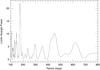 |
Fig. 10 L-S periodogram of the bisector span measurements. |
5.4. Bisector variations
Spectral line bisectors have become a common tool to ensure that RV variations attributed to orbital motion are not in fact due to intrinsic stellar variations (Hatzes et al. 1998; Queloz et al. 2001). We thus examined the bisectors using the McD-Tull data set. This was selected because we wanted to use a consistent data set in measuring the bisectors. The McD-Tull data has the longest time baseline and a pipeline has been developed for measuring bisectors from this instrument. Although the BOAO data has the highest resolution, the BOES has an unstable instrument profile that is modeled in calculating the RVs, but is not accounted for in any bisector measurements.
In our analysis we used a statistical approach in order to select the “cleanest” lines for calculating the bisector. First, we identified those spectral lines that were relatively deep and that appeared to be free from nearby blends in the wavelength region 4000−10 000 Å. We ignored lines in the spectral regions 4610−4760 Å, 6830−6940 Å, 7590−7720 Å, and 8130−8270 Å, as well as smaller regions containing telluric lines. A linear fit to each side of the spectral line and a Gaussian fit to the line core was performed. Next we examined the deviation of the fit parameters from individual lines from that of the average values. A large deviation indicated that a line was strongly affected by a blend and this line was removed from the analysis. We then computed the bisector for each the final selection of 75 spectral lines. The bisector velocity span was calculated using the difference of the average bisector values between flux levels of 0.1−0.3 and 0.7−0.9 of the continuum value. Finally, the individual bisector span measurements were combined to produce an average bisector velocity span.
Figure 10 shows the L-S periodogram of the bisector span measurements. No significant peak is found at the 629 d period. However, a significant peak is found at a period, P = 175.4 ± 0.6 d which is 1/3 the period found in the CaII S-index and Hα measurements. A bootstrap analysis yields a FAP < 5 × 10⁻⁶ for this signal.
5.5. Residual RV variations
The activity indicators of Hα and Ca II K show variations with a period of ≈520 d that are most likely caused by rotational modulation of surface features from stellar active regions. We suspect that such a period in the RVs may be responsible for the poor fits to the orbital solution in some years.
Figure 11 shows the residual RV variations after subtracting the orbital solution. Note the sine-like variations between 2003 and 2004 (JD-2 400 000 = 52 500−53 600), the same time where the orbital fit is poor. Figure 12 shows the L-S periodograms of the residual RV data prior to (top) and after (middle) JD = 2 450 000. The lower panel shows the periodogram of all the residuals.
The behavior of the L-S periodogram suggests that this period is not long-lived. Different peaks become more prominent as more data is added, and more importantly the L-S power does not dramatically increase in the combined data sets, unlike the 629 d period. The RV residuals prior to JD = 2 4500 00 show the strongest power, z, at P = 598 d and P = 518 d (z = 12.7 and 9.7, respectively). The RV residuals after JD = 2 450 000, on the other hand, show the most power at P = 715 d and P = 538 d (z = 16.5 and 15.8, respectively). The combined data show the strongest peak at P = 542 d, z = 18.4. If this were a coherent and long-lived signal, then it should have been detected with higher significance. A simulated periodic signal with P = 540 d and K = 100 m s-1 and σ = 100 m s-1 was generated and sampled in the same way as the data. A periodogram analysis revealed that the signal was easily detected in just the first half of the data (z = 20) and was highly significant in the full data set (z = 60).
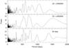 |
Fig. 12 L-S periodograms of the residual RV data after removing the orbital solution. The top panel is from data prior to JD = 2 450 000, the middle panel for data afterwards, and the bottom panel for all data. |
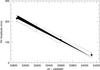 |
Fig. 13 K-amplitude of the 521 d period seen in the RV residuals as a function of time. |
A visual inspection of the time series residuals also indicates that the ~500 d variations are not long lived. There are strong variations at JD ≈ 2 453 000 that clearly fade away by JD ≈ 2 454 000. To investigate this possible amplitude variation we divided the residual RV data taken between 2002.8 and 2008.3 into four sliding subsets in time with widths of ~2−2.5 yr and found the best fit K-amplitude using the 521 d period. The K-amplitude decreases from about 200 m s-1 to 40 m s-1 in about 3.5 yr (Fig. 13).
Although this signal is not long-lived, there are other instances when it appears at other epochs. We divided the RV residual data into three subset epochs: “Epoch 1”, JD = 2 444 531−2 446 726 (1980.8−1986.8), “Epoch 2”, JD = 2 448 831−2 450 000 (1992.6−1993.6), and “Epoch 3”, JD = 2 453 253−2 454 396 (2004.7−2008.2). These three epochs showed the largest variations in the RV residuals. A period search was then performed in each epoch. In Epoch 3 the RV residuals were best fit with P = 521 ± 11 d, and a K-amplitude of 95 ± 10 m s-1. In Epoch 2 the best fit was with P = 526 ± 82 d, K = 132 ± 30 m s-1. The data were too sparse in Epoch 1 for a reliable fit; however, when combining the data from all three epochs a good fit was obtained with P = 534.7 ± 1.7 d, and K = 91.2 ± 9.0 m s-1. Figure 14 shows the residual RV variations of the three epochs phased to the 534.7 d period. Although this signal appears intermittently in the data, it appears to phase well with other epochs.
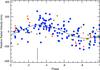 |
Fig. 14 Residual RV variations phased using a best-fit period of 534.7 d for three epochs: 1980.8−1986.8 (triangles), 1992.6−1993.6 (squares), and 2004.7−2008.2 (dots). The vertical line indicates the peak-to-peak RV variations due to the stellar oscillations. |
We should note that the peak in the L-S periodogram for the residual RVs spanning for Epoch 3, 2004.7−2008.2 (lower panel of Fig. 9), coincides exactly with the one found in the Ca II S-index and Hα measurements over the same time span.
Table 11 summarizes the periods found by the analysis of the activity indicators and the residual RV data.
Periods derived from RV residuals and activity indicators.
6. Discussion
Our new radial velocity measurements for α Tau when combined withprevious published data show that the ~645 d RV variations found by HC93 are indeed long-lived and coherent. A careful examination of the Ca II K emission, spectral line shapes and Hipparcos photometry reveals no convincing variation with the 629 d RV period. A previous study by Hatzes & Cochran (1998) established that there were no spectral line shape variations (line bisectors) with the 629 d RV period. All of these support the fact that the RV variations at this period are due to the planet hypothesis first proposed by HC93.
The analysis of the ancillary data of residual RVs, Ca II K S-index, and Hα reveals the presence of a ≈520 d period that seemed to be only in the residual RV data taken between 2004.7 and 2008.2, the early McDonald and DAO data (1992.6−1993.6), and possibly the CFHT data (1980.8−1986.8). This period is not present in the RV data or Ca II 8662 Å measurements made prior to 2000. We interpret this signal as due to rotational modulation by stellar surface structure. The amplitude variations (Fig. 13) can be explained by the evolution of surface spot features. A reasonable explanation for the absence of the signal in some years is an activity cycle. If indeed the ~520 d period is due to rotation then this provides further support to the 629 d RV period arising from Keplerian motion from a companion.
One could argue that both the 629 d period seen in the RV data and the 520 d period seen in the residual RVs and activity indicators are all due to rotation and we are seeing the effect of differential rotation. However, if the 629 d period is also due to rotational modulation, then we should have at least some evidence of its presence in the activity indicators or the line bisector measurements of Hatzes & Cochran (1998) as is the case for the 520 d period. Stellar surface structure that cause RV variations should also produce variations in at least one of these other quantities.
If indeed the two periods are due to differential rotation then we can estimate the differential rotation parameter, α = (ωpole−ωequator)/ωequator where ωpole and ωequator are the polar and equatorial rotational angular velocities. Taking our two periods as the polar and equatorial rotational periods results in α≥ 0.2, or greater than the solar value of α = 0.14. The value of α could be considerably larger if the one of the periods represents a mid-latitude rotational period rather than the polar one. This large value of differential rotation should result in strong stellar activity, but our Ca II and Hα measurements suggest a relatively low level of activity for this star.
However, recent work by Küker & Rüdiger (2012) on the K giant star KIC 8366239 predicted a solar type differential rotation in this star, so modest amount of differential rotation in K giant stars may be possible. Looking at the RV variations between 2003 and later, if one were to explain the long-period RV variations of α Tau, then you require a spot feature to form in 2003 at a latitude where the rotational period is ~500 d. This spot would quickly (Δt ≈ 1 yr) have to migrate to another latitude that has rotational period of 630 d. It would then have to be stable in size and location for the next eight years. Given our limited knowledge of activity in K giant stars this may be possible, but seems less plausible than having a sub-stellar companion and rotational modulation.
The spectral line bisector variations show no significant variations at either the orbital period of the planet or the ≈520 d variations that we attribute to the rotation of the star. However, there is a significant peak at a period of 175 d. Interestingly, this is one-third the period found in the RV residuals and the activity indicators (Table 11). The most logical explanation for this period is that it is the third harmonic of the stellar rotation period, i.e. Prot/3.
It is not clear why we see variations in the bisectors at third harmonic of the rotational period. Naively, one expects that the variations in spectral line shapes (bisectors) are directly tied to the RV variations and that one should at least see evidence of Prot in the bisectors. However, we should stress that we know little about the nature of the activity related structure (e.g. starspots) and the velocity field (e.g. convection) on the surface of giant stars and how these influence both the line shapes and the integrated RV measurements. It may be that a harmonic of the rotational period is only seen in one quantity. Alternatively, the lack of power at Prot in the periodogram of the bisector variations may be due to a combination of the real variations, the sampling, and the noise characteristics of the bisector measurements.
There is evidence, however, of a harmonic of the rotational period in a K giant star being present in some observed quantities. In a pioneering study of the He I 10830 Å line in Arcturus, Lambert (1987) found evidence for a 78 d variation in this activity indicator. Lambert argued that the He I variations represent one-third of the actual stellar rotational period of 233 d. Subsequently, HC93 found evidence of an RV period of 231 d in Arcturus, nearly identical to the inferred rotational period. Unlike α Tau and β Gem, the long period variations in Arcturus found by HC93 are most likely due to rotational modulation.
Spectral line bisector measurements have become a standard tool for confirming planets around giant stars. The assumption is that if one sees no variations in the bisectors, or variations at a different period to the RV period, then the RV variations must be due to a planet. In the case of α Tau, one sees periodic bisector variations different to the 520 d residual RV period, but at a harmonic. The measurements of activity indicators show, however, that the residual RV and bisector periods can be interpreted in a consistent way if one assumes that they are all related to the rotational period of the star. There are other instances where harmonics of the rotational period of the star have masqueraded as an RV signal believed to be due to a planet (Robertson et al. 2014). In confirming planets around giant stars it is wise to examine all available activity indicators.
The residual RVs show indications for an activity cycle in α Tau. These show an active phase that lasts approximately 3.5 yr (Fig. 13) after which the star enters a quiet phase. The activity-related RV variations were strongest in 2003−2005, 1993, and possibly around 1984 judging by the large residual variations in the CFHT data. This implies an activity cycle of ≈ 10 yr. However, given the sometimes large gaps in our RV coverage, this time scale is only a crude estimate. Interestingly, this is near the period seen in the long-term variations in the S-index (Fig. 8). The decay in the RV amplitude shown in Fig. 14 indicates a “spot” lifetime of ≈3.5 yr.
It is not known what the nature of the activity is on a K giant, whether these are cool spots, or possibly large convection cells organized by magnetic fields. The variations seen in the traditional indicators such as Hα suggest this activity is analogous to solar magnetic activity. The fact that subsets of the residual RV data separated by about ten years phase well when using the same period (Fig. 14) suggests that this activity may occur in active longitudes on the star. Dedicated RV monitoring of K giant stars with better temporal sampling may provide valuable clues to stellar activity on evolved stars.
All the available evidence suggests that the 629 d RV variations in α Tau are most likely caused by Keplerian motion of a companion. The additional ~520 d period that is short lived and not coherent is due to rotational modulation of active regions.
Our value of 1.13 M⊙ for the stellar mass results in a minimum companion mass of 6.47 ± 0.53 MJup. The substellar companion to α Tau has similar properties to other companions around giant stars. These are mostly “super planets” in the mass range 3−14 MJup and with orbital radii of ≈2 AU (Hatzes 2008).
Our RV and ancillary measurements for α Tau demonstrate that K giant stars can have sub-stellar companions and stellar surface structure, both of which show up as long (several hundreds of days) periods. This presents a cautionary tale for programs searching for planets around evolved stars with the RV method. Our residual RV measurements show evidence for variations with a 520−540 d period and a K-amplitude of ≈100 m s-1. This is comparable to the amplitudes and periods found in the RV variations of other K giant stars. If you had poor temporal sampling and were to phase the residual RV from approximately a decade earlier, the results would suggest a long-lived coherent RV signal consistent with a planetary companion having a minimum mass of approximately 8 MJup. The L-S periodogram of the data when this signal was present yields power at this period consistent with a FAP ≈ 10-10. A bootstrap analysis yields a FAP < 5 × 10⁻⁶. However, this “planetary-like” signal disappears with more data having better sampling.
One should be cautious in interpreting RV variations as due to companions in giant stars. This is especially true when one does not have the luxury of three decades of data to establish longevity of the RV signal, a primary requirement for a planetary signal. Looking at ancillary measurements of activity indicators (Hα, Ca II, photometry, line shapes, etc.) is necessary to confirm signals from companions. In particular, it appears that Hα is a suitable diagnostic of activity variations. Clearly, K giant stars represent a fertile ground not only for discovering exoplanets, but also for investigating stellar activity in evolved stars.
Acknowledgments
The authors wish to thank the referee, Martin Kürster, for his very careful reading of the manuscript and for making suggestions that greatly improved the paper. Referees like him are greatly appreciated. A.P.H. and M.D. acknowledge grant HA 3279/8-1 from the Deutsche Forschungsgemeinschaft (DFG). WDC acknowledges the support of NASA grants NNG04G141G and NNG05G107G. W.D.C., M.E., and P.M. acknowledge support from grant AST-1313075 from the National Science Foundation. G.A.H.W. is supported by the Natural Sciences and Engineering Research Council of Canada. A.E.S. gratefully acknowledges partial funding from the Sciex Programme of the Rector’s Conference of the Swiss Universities. We also thank the many observers of the McDonald Observatory planet search program that have helped to obtain the extensive α Tau data: Paul Robertson, Erik Brugamyer, Rob Wittenmyer, Kevin Gullikson, Ivan Ramirez, Marshall Johnson, Caroline Caldwell, Diane Paulson and Candace Gray. This research has made use of the SIMBAD data base operated at CDS, Strasbourg, France.
References
- Campbell, B., & Walker, G. A. H. 1979, PASP, 91, 540 [NASA ADS] [CrossRef] [Google Scholar]
- Cochran, W. D., Hatzes, A. P., Butler, R. P., & Marcy, G. W. 1997, ApJ, 483 [Google Scholar]
- da Silva, L., Girardi, L., & Pasquini, L., et al. 2006, A&A, 458, 609 [NASA ADS] [CrossRef] [EDP Sciences] [Google Scholar]
- Döllinger, M., Hatzes, A., Pasquini, L., et al. 2007, A&A, 472, 649 [NASA ADS] [CrossRef] [EDP Sciences] [Google Scholar]
- Endl, M., Hatzes, A. P., Cochran, W. D., et al. 2004, ApJ, 611, 1121 [NASA ADS] [CrossRef] [Google Scholar]
- Frink, S., Mitchell, D. S., Quirrenbach, A., et al. 2002, ApJ, 576, 478 [NASA ADS] [CrossRef] [MathSciNet] [Google Scholar]
- Gustafsson, B., Bell, R. A., Eriksson, K., & Nordlund, A. 1975, A&A, 42, 407 [NASA ADS] [Google Scholar]
- Han, I., Lee, B-C., Kim, K.-M., & Mkrtichian, D. E. 2008, J. Korean Astron. Soc., 41, 59 [Google Scholar]
- Hatzes, A. P. 2008, Phys. Scr., 130, 4004 [Google Scholar]
- Hatzes, A. P., & Cochran, W. D. 1993, ApJ, 413, 339 (HC93) [NASA ADS] [CrossRef] [Google Scholar]
- Hatzes, A. P., & Cochran, W. D. 1994, ApJ, 422, 366 [NASA ADS] [CrossRef] [Google Scholar]
- Hatzes, A. P., & Cochran, W. D. 1998, MNRAS, 293, 469 [NASA ADS] [CrossRef] [Google Scholar]
- Hatzes, A. P., Cochran, W. D., & Bakker, E. J. 1998, Nature, 391, 154 [NASA ADS] [CrossRef] [Google Scholar]
- Hatzes, A. P., Guenther, E. W., Endl, M., et al. 2005, A&A, 437, 743 [NASA ADS] [CrossRef] [EDP Sciences] [Google Scholar]
- Hatzes, A. P., Cochran, W. D., Endl, M., et al. 2006, A&A, 457, 335 [NASA ADS] [CrossRef] [EDP Sciences] [Google Scholar]
- Jefferys, W., Fitzpatrick, J., & McArthur, B. 1988, Celest. Mech. 41, 39 [Google Scholar]
- Jørgensen, B. R., & Lindegren, L. 2005, A&A, 436, 127 [NASA ADS] [CrossRef] [EDP Sciences] [Google Scholar]
- Kim, K. M., Mkrtichian, D. E., Lee, B.-C., Han, I., & Hatzes, A. P. 2006, A&A, 454, 839 [NASA ADS] [CrossRef] [EDP Sciences] [Google Scholar]
- Kovacs, N. 1983, A&A, 120, 21 [NASA ADS] [Google Scholar]
- Küker, M., & Rüdiger, G. 2012, Astron. Nachr., 333, 1028 [NASA ADS] [CrossRef] [Google Scholar]
- Kürster, M., Schmitt, J. H. M. M., Cutispoto, G., & Dennerl, K. 1997, A&A, 320, 831 [NASA ADS] [Google Scholar]
- Kürster, M., Endl, M., Rousenal, F., et al. 2003, A&A, 403, 1077 [NASA ADS] [CrossRef] [EDP Sciences] [Google Scholar]
- Lambert, D. L. 1987, ApJS, 65, 255 [NASA ADS] [CrossRef] [Google Scholar]
- Larson, A. M., Irwin, A. W., Yang, S. L. S., et al. 1993a, PASP, 105, 332 [NASA ADS] [CrossRef] [Google Scholar]
- Larson, A. M., Irwin, A. W., Yang, S. L. S., et al. 1993b, PASP, 105, 825 [NASA ADS] [CrossRef] [Google Scholar]
- Lomb, N. R. 1976, Ap&SS, 39, 447 [NASA ADS] [CrossRef] [Google Scholar]
- Luck, R. E., & Challener, S. L. 1995, AJ, 110, 2968 [NASA ADS] [CrossRef] [Google Scholar]
- McWilliam, A. 1990, ApJS, 74, 1075 [NASA ADS] [CrossRef] [Google Scholar]
- Murdoch, K. A., Hearnshaw, J. B., & Clark, M. 1993, ApJ, 413, 349 [NASA ADS] [CrossRef] [Google Scholar]
- Niedzielski, A., Nowak, G., Adamów, M., & Wolszczan, A. 2009, ApJ, 707, 768 [NASA ADS] [CrossRef] [Google Scholar]
- Queloz, D., Henry, G. W., Sivan, J. P., et al. 2001, A&A, 379, 279 [NASA ADS] [CrossRef] [EDP Sciences] [Google Scholar]
- Queloz, D., Bouchy, F., & Moutou, C. 2009, A&A, 506, 303 [NASA ADS] [CrossRef] [EDP Sciences] [Google Scholar]
- Reffert, S., Quirrenbach, A., Mitchell, S., et al. 2006, ApJ, 652, 661 [NASA ADS] [CrossRef] [Google Scholar]
- Richichi, A., & Roccatagliata, V. 2005, A&A, 433, 305 [NASA ADS] [CrossRef] [EDP Sciences] [Google Scholar]
- Robertson, P., Endl, M., Cochran, W. D., et al. 2012, ApJ, 749, 39 [NASA ADS] [CrossRef] [Google Scholar]
- Robertson, P., Mahadevan, S., Endl, M., & Roy, A. 2014, Science, 345, 440 [NASA ADS] [CrossRef] [Google Scholar]
- Scargle, J. D. 1982, ApJ, 263, 835 [NASA ADS] [CrossRef] [Google Scholar]
- Setiawan, J., Hatzes, A. P., von der Lühe, O., et al. 2003, A&A, 398, L19 [NASA ADS] [CrossRef] [EDP Sciences] [Google Scholar]
- van Leeuwen, F. 2007, Hipparcos, the New Reduction of the Raw Data, Astrophys. Space Sci. Lib., 350 [Google Scholar]
- Walker, G. A. H., Yang, S. L. S., Campbell, B., & Irwin, A. W. 1989, ApJ, 343, L21 [NASA ADS] [CrossRef] [Google Scholar]
All Tables
All Figures
|
Fig. 1 Probability density functions (PDF) for various parameters of α Tau. The histogram (on right) for each row shows the PDF for (top to bottom) stellar age, mass, radius, and surface gravity. The correlation plots on each row show how that parameter correlates with the other parameters. |
| In the text | |
|
Fig. 2 Radial velocity measurements for α Tau from the seven data sets: CFHT (diamonds), DAO (inverted triangles), McD-2.1 m (circles), McD-CS11 (squares), McD-Tull (sideways triangles), TLS (triangles), and BOAO (pentagons). Zero point corrections have been applied to the individual data sets before plotting (see text). The curve represents the orbital solution (see Table 10). The vertical dash represents the peak-to-peak variations of the stellar oscillations. |
| In the text | |
|
Fig. 3 L-S periodogram of the RV measurements taken prior to JD = 2 450 000 (top), after JD = 2 450 000 (middle), and the full data set (bottom). |
| In the text | |
|
Fig. 4 Radial velocity measurements for α Tau from the seven data sets phased to the orbital period.For the TLS and McD-Tull data we plot run-binned averages that were used in the orbital solution. The solid line is the orbital solution and the vertical line the peak-peak short term intrinsic RV variations observed for this star. Symbols are the same as for Fig. 2. Error bars for individual measurements are not shown for clarity and because the scatter is dominated by the intrinsic stellar variability. |
| In the text | |
|
Fig. 5 L-S power (z) of the 629 d period as a function of the number of data points used in the periodogram calculation (circles). The power, z, as a function of the number of data points for simulated data (triangles). |
| In the text | |
|
Fig. 6 Hipparcos photometry phased to the 629 d orbital period. |
| In the text | |
|
Fig. 7 L-S periodogram of the ΔEW8662 variations. |
| In the text | |
|
Fig. 8 Variations of the McDonald S-index measurements with time. The line represents a sine fit with a period P = 4320 ± 450 d. |
| In the text | |
|
Fig. 9 Top to bottom: L-S periodograms of the McDonald S-index, Hα equivalent width, Hα FWHM, and residual RV measurements. The RV residuals were taken from the time interval 2004.7−2008.2 (see text). |
| In the text | |
|
Fig. 10 L-S periodogram of the bisector span measurements. |
| In the text | |
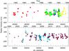 |
Fig. 11 Residual RV variations for α Tau after subtracting the orbital solution of Table 10. |
| In the text | |
|
Fig. 12 L-S periodograms of the residual RV data after removing the orbital solution. The top panel is from data prior to JD = 2 450 000, the middle panel for data afterwards, and the bottom panel for all data. |
| In the text | |
|
Fig. 13 K-amplitude of the 521 d period seen in the RV residuals as a function of time. |
| In the text | |
|
Fig. 14 Residual RV variations phased using a best-fit period of 534.7 d for three epochs: 1980.8−1986.8 (triangles), 1992.6−1993.6 (squares), and 2004.7−2008.2 (dots). The vertical line indicates the peak-to-peak RV variations due to the stellar oscillations. |
| In the text | |
Current usage metrics show cumulative count of Article Views (full-text article views including HTML views, PDF and ePub downloads, according to the available data) and Abstracts Views on Vision4Press platform.
Data correspond to usage on the plateform after 2015. The current usage metrics is available 48-96 hours after online publication and is updated daily on week days.
Initial download of the metrics may take a while.