| Issue |
A&A
Volume 579, July 2015
|
|
|---|---|---|
| Article Number | A36 | |
| Number of page(s) | 19 | |
| Section | Planets and planetary systems | |
| DOI | https://doi.org/10.1051/0004-6361/201424501 | |
| Published online | 23 June 2015 | |
Transiting exoplanets from the CoRoT space mission ⋆,⋆⋆
XXVII. CoRoT-28b, a planet orbiting an evolved star, and CoRoT-29b, a planet showing an asymmetric transit
1
Institute of Planetary Research, German Aerospace
Center, Rutherfordstrasse
2, 12489
Berlin,
Germany
e-mail: This email address is being protected from spambots. You need JavaScript enabled to view it.
2
Institut d’Astrophysique de Paris, UMR 7095 CNRS, Université
Pierre & Marie Curie, 98bis
boulevard Arago, 75014
Paris,
France
3
Leiden Observatory, University of Leiden,
PO Box 9513, 2300 RA, Leiden, The Netherlands
4
Department of Earth and Space Sciences, Chalmers University of
Technology, Onsala Space Observatory, 439 92
Onsala,
Sweden
5
Max Planck Institute for Astronomy Königstuhl 17,
69117
Heidelberg,
Germany
6
Thüringer Landessternwarte, Sternwarte 5, 07778
Tautenburg,
Germany
7
LESIA, UMR 8109 CNRS, Observatoire de Paris, UPMC, Université
Paris-Diderot, 5 place J.
Janssen, 92195
Meudon,
France
8
Aix Marseille Université, CNRS, LAM (Laboratoire d’Astrophysique
de Marseille) UMR 7326, 13388
Marseille,
France
9
IAG-Universidade de Sao Paulo, 05508-090
Sao Paulo,
Brasil
10
Zentrum für Astronomie, Fakultät für Physik und
Astronomie, Mönchhofstr.
12-14, 69120
Heidelberg,
Germany
11
Université de Nice-Sophia Antipolis, CNRS UMR 6202, Observatoire
de la Côte d’Azur, BP
4229, 06304
Nice Cedex 4,
France
12
Österreichische Akademie der Wissenschaften, Institut für
Weltraumforschung, IWF,
Schmiedlstraße 6, 8042
Graz,
Austria
13
Instituto de Astrofísica de Canarias, 38205, La
Laguna, Tenerife, Spain
14
Dept. Astrofísica, Universidad de la Laguna,
38206, La Laguna, Tenerife,
Spain
15
Sub-department of Astrophysics, Department of Physics, University
of Oxford, Oxford,
OX1 3RH,
UK
16
Rheinisches Institut fürUmweltforschung an der Universität zu
Köln, 50931
Aachener Strasse 209,
Germany
17
University of Hawaii, Institute for Astronomy,
34 Ohia Ku Street, Pukalani, Hawaii
96768,
USA
18
Las Cumbres Observatory Global Telescope Network,
Inc. 6740 Cortona Drive Suite
102, Goleta,
CA
93117,
USA
19
INAF–Osservatorio Astrofisico di Torino,
via Osservatorio 20,
10025
Pino Torinese,
Italy
20
LAB, UMR 5804, Univ. Bordeaux & CNRS,
33270
Floirac,
France
21
Institut d’Astrophysique Spatiale, Université Paris-Sud &
CNRS, 91405
Orsay,
France
22
Max-Planck-Institut für extraterrestrische Physik,
Giessenbachstrasse 1,
85748
Garching,
Germany
23
Torrance High School, 2200 W Carson St, Torrance, CA
90501,
USA
24
Observatoire de l’Université de Genève,
51 chemin des Maillettes,
1290
Sauverny,
Switzerland
25
University of Vienna, Institute of Astronomy,
Türkenschanzstr. 17,
1180
Vienna,
Austria
26
Iolani School, 563 Kamoku St., Honolulu, HI-96816, USA
27
School of Physics and Astronomy, Raymond and Beverly Sackler
Faculty of Exact Sciences, Tel Aviv University, 6997801
Tel Aviv,
Israel
28
CFHT Corporation, 65-1238 Mamalahoa Hwy,
Kamuela, Hawaii
96743,
USA
29
Institut für Astrophysik, Friedrich-Hund-Platz 1, 37077
Göttingen,
Germany
30
Center for Astronomy and Astrophysics, TU Berlin, Hardenbergstr.
36, 10623
Berlin,
Germany
31
Instituto de Astrofísica e Ciências do Espaço, Universidade do
Porto, CAUP, Rua das
Estrelas, 4150-762
Porto,
Portugal
32
LUTH, Observatoire de Paris, UMR 8102 CNRS, Université Paris
Diderot, 5 place Jules
Janssen, 92195
Meudon,
France
Received: 30 June 2014
Accepted: 30 March 2015
Abstract
Context. We present the discovery of two transiting extrasolar planets by the satellite CoRoT.
Aims. We aim at a characterization of the planetary bulk parameters, which allow us to further investigate the formation and evolution of the planetary systems and the main properties of the host stars.
Methods. We used the transit light curve to characterize the planetary parameters relative to the stellar parameters. The analysis of HARPS spectra established the planetary nature of the detections, providing their masses. Further photometric and spectroscopic ground-based observations provided stellar parameters (log g, Teff, v sin i) to characterize the host stars. Our model takes the geometry of the transit to constrain the stellar density into account, which when linked to stellar evolutionary models, determines the bulk parameters of the star. Because of the asymmetric shape of the light curve of one of the planets, we had to include the possibility in our model that the stellar surface was not strictly spherical.
Results. We present the planetary parameters of CoRoT-28b, a Jupiter-sized planet (mass 0.484 ± 0.087 MJup; radius 0.955 ± 0.066 RJup) orbiting an evolved star with an orbital period of 5.208 51 ± 0.000 38 days, and CoRoT-29b, another Jupiter-sized planet (mass 0.85 ± 0.20 MJup; radius 0.90 ± 0.16 RJup) orbiting an oblate star with an orbital period of 2.850 570 ± 0.000 006 days. The reason behind the asymmetry of the transit shape is not understood at this point.
Conclusions. These two new planetary systems have very interesting properties and deserve further study, particularly in the case of the star CoRoT-29.
Key words: planetary systems / techniques: photometric / techniques: radial velocities / techniques: spectroscopic
The CoRoT space mission, launched on December 27th 2006, was developed and is operated by CNES, with the contribution of Austria, Belgium, Brazil, ESA (RSSD and Science Programme), Germany, and Spain. Based on observations obtained with the Nordic Optical Telescope, operated on the island of La Palma jointly by Denmark, Finland, Iceland, Norway, and Sweden, in the Spanish Observatorio del Roque de los Muchachos of the Instituto de Astrofisica de Canarias, in time allocated by OPTICON and the Spanish Time Allocation Committee (CAT). The research leading to these results has received funding from the European Community’s Seventh Framework Programme (FP7/2007-2013) under grant agreement number RG226604 (OPTICON). This work makes use of observations from the LCOGT network.
Appendices are available in electronic form at http://www.aanda.org
© ESO, 2015
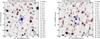 |
Fig. 1 Second Palomar Observatory Sky Survey (POSS II, Reid et al. 1991) image around the CoRoT-28 (left) and CoRoT-29 (right) targets. We have over-plotted the CoRoT masks used in the observations and we give identification labels for the brightest, closest background stars. The mask of CoRoT-28 shows the subdivision in the three submasks, named from north to south: red, green, and blue. |
1. Introduction
Spaceborne surveys of transiting extrasolar planets like CoRoT (Baglin et al. 2006) or Kepler (Borucki et al. 2010) have provided crucial evidence of the interactions between stars and planets and their common evolution. In this paper we report the discovery and characterization of two systems with interesting properties.
CoRoT-28b is a hot Jupiter orbiting an evolved star. We investigated the stellar and planetary properties, in particular the rotation and metallicity of the star, and found a lithium abundance higher than expected for its evolutionary state.
CoRoT-29b is a bit of a riddle. The transit discovered by CoRoT is significantly asymmetric, a signature that the host star could have a non-spherical shape. The asymmetry measured by CoRoT has been confirmed by ground-based observations at several observatories. We developed a code that successfully models the transit light curve assuming that the star is oblated. The deformation of the star implied by our model, however, is far too large compared to our current understanding of stellar interiors. Other possible scenarios are bands of stellar spots on the surface of the star, which if properly placed, could also reproduce the transit light curve measured. We show the observational evidence and our modelling efforts, but we leave open the question of the origin of the asymmetry.
2. CoRoT observations and data reduction
2.1. General description
The satellite CoRoT observed the field LRc08 (pointing coordinates 18h 28m 34.7s, 5°36′0.0′′) in 2011 between 6 July and 30 September. The CoRoT data for the run LRc08 has been public since 7 June 2013 and can be obtained through the IAS CoRoT Archive1.
IDs, coordinates, and magnitudes of CoRoT-28 and CoRoT-29.
The coordinates, identification labels, and magnitudes of the stars CoRoT-28 and CoRoT-29 are given in Table 1. CoRoT-28 is a relatively bright target and it was assigned an observing cadence rate of 32 s from the start of the observations, collecting 225 087 measurements with a chromatic mask. CoRoT-29 is a fainter target and was assigned the cadence rate of 512 s. When the first transits were discovered by the Alarm Mode, the target was assigned a sampling rate of 32 s, collecting in total 121 288 measurements with a monochromatic mask. The region around both targets, indicating the position of the nearest contaminants and the orientation of the masks, is shown in Fig. 1. For an overview of the CoRoT observing modes, please refer to Boisnard & Auvergne (2006), Barge et al. (2008), Auvergne et al. (2009).
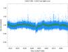 |
Fig. 2 Raw light curve of CoRoT-28. The original data points, sampled at 32 s, are shown in blue. We have binned the data to 512 s bins to guide the eye. |
2.2. CoRoT-28b
The raw light curve of CoRoT-28 is shown in Fig. 2. We treated the EN2 level2 light curve of CoRoT-28 observed by CoRoT in its version 3.0. The removal of the influence of instrumental systematics and stellar variability is a necessary step before obtaining the planetary parameters from the light-curve fit. Standard methods consist in the subtraction of a low-level polynomial (in our case, a parabola) to an interval around each transit with a length of a few transit durations (in our case, three). This method was applied successfully with the light curve of CoRoT-28, and we then proceeded to the modelling of the planetary parameters as described in Sect. 4.1.
2.3. CoRoT-29b
In the case of CoRoT-29, the standard reduction procedures described in Sect. 2.2 revealed a feature with the shape of non-zero slope in the bottom of the transit shape, which is otherwise expected to be reasonably flat. The slope of the bottom part of the transit is non-zero with 95% confidence level in the 32 s sampled data by CoRoT, and only non-zero with 1σ significance in the 512 s sampled data set. But at the same time, CoRoT-29 is a fainter star than CoRoT-28 and its light curve has more noise at the timescales comparable with the transit length. We therefore decided to use a more robust filtering for this light curve.
We followed the procedure described in Alapini & Aigrain (2009), which iteratively fits the planetary parameters, subtracts the planetary model from the data, creates a model of the stellar variability, then subtracts the stellar variability model from the original data, and then fits the planetary parameters again until the method converges to a final set of planetary parameters and stellar activity pattern. In the first iteration, we used a sliding time window of 0.5 days in length to deal with the variations due to activity. For the interpolation, we removed the points measured during the transit. But for the next iteration steps we divided the light curve in intervals of 0.5 days and fitted each interval with a Legendre polynomials of order 5. This was chosen because a sliding window with short timescales might have an influence on sharp features in the light curve, such as the transit ingress or egress, and the method might fail to converge (see also the discussion in Bonomo et al. 2012).
We tried with intervals from 0.5 to 1.5 days in steps of 0.1 days and though the removal of the systematics is not equally satisfactory for each interval, the non-zero slope in the bottom transit of CoRoT-29b remained. A Legendre polynomial of order 5 within a 0.5 day window provides a smooth fit to the data and it is able to remove the contributions from the out-of-transit, spot-induced stellar activity and low-frequency instrumental systematics present in the data. The regions of the light curve sampled at 512 s and at 32 s were treated as independent data sets. Our method converged after three iterations (one with the sliding window and two with the Legendre polynomials, see Fig. 3).
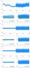 |
Fig. 3 Iterative filtering applied to the light curve of CoRoT-29b, converging in three steps (labelled A, B, and C). Top of each panel shows the light curve (normalized flux vs. CoRoT Julian Date, which is HJD − 2 451 545.0), the bottom figures on each panel show the folded light curves (normalized flux vs. orbital phase). |
2.4. Background correction of CoRoT-29b
Comparing the transits of the section of the CoRoT light curve sampled at 512 s and at 32 s, we were able to identify a change in the observed transit depth, which required further study (see Fig. 4). Auvergne et al. (2009) described the photometric capabilities of the CoRoT satellite in detail. However some of those capabilities have slightly degraded with the ageing of the instrument. One effect is the increase of the dark current of the CCD, which has an important impact on the on-board photometry. The dark current of the CCD was modelled as a uniform value calculated in 196 (14 × 14) windows distributed along the CCD: 3/4 of them sampled at 512 s and 1/4 of them sampled at 32 s. The correction applied to the 32 s and 512 s light curves was the median value of the 32 s and 512 s background windows, respectively, to mitigate the impact of hot pixels and cosmic ray impacts. However, with the ageing of the CCD, the uniform model for the dark current is no longer a faithful description of the phenomenon. We observed a gradient along the Y axis of the CCD whose slope has increased with time. Moreover, the distribution of background windows sampled at 512 s and 32 s is not uniform, which introduces an additional bias in the background correction. The median background level at 32 s sampling is calculated in a region of the CCD that has in average a lower Y value than the average of the windows sampled at 512 s, which introduces a visible difference in the mean level of the light curve at the two different sampling rates. This effect is common to all light curves on the CCD during this particular run, but it cannot be seen in the light curve of CoRoT-28, as this target was only sampled at the 32 s cadence. This effect can be mitigated by modifying the corresponding background correction for each star as a function of its position on the CCD, a feature that will be introduced in future releases of CoRoT data.
The CoRoT pipeline is currently implementing an improved background correction to mitigate this effect. We used the data of this improved pipeline (version 3.53). However, the final planetary parameters determined when using the previous (version 3.0) or the new data (version 3.5) are not significantly different. Our modelling fits the background contamination as a free parameter, and can deal with the residuals left by the background correction from the pipeline. The incomplete background correction pipeline dilutes the transit signal as if there was an additional contribution of light from a background star, a well-known effect that can be corrected with standard procedures.
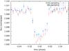 |
Fig. 4 Change in the transit depth of CoRoT-29b observed in the light curves sampled at 512 s and 32 s (version 3.0 of the data). |
3. Ground-based observations
The main objective of ground-based photometric follow-up is to check whether the observed transit features occur on the target star or might arise on a nearby eclipsing-binary system (Deeg et al. 2009). Then, ideally, low-resolution spectroscopic measurements characterize the nature of the stellar target before high-resolution radial velocity measurements independently confirm the planetary nature of the target providing a value of its mass (Moutou et al. 2009). This section describes the ground-based observations carried out to characterize these CoRoT targets.
3.1. Photometric measurements
CoRoT-28b
Photometric follow-up of CoRoT-28b was performed with the IAC80 (Tenerife) and the Euler (La Silla) telescopes. Photometric data were acquired at the 80 cm telescope of the IAC on Tenerife (IAC80). Measurements during the transit (on) obtained on 9 October 2011 and out-of-transit (off) data taken on 25 October 2011 showed an on-off brightness variation of 0.3%, but at a low level of confidence. Each observing run lasted 33 minutes. Conversely, relevant brightness variations could be excluded with high confidence on the neighboring stars (stars 2, 3, 6, 13, and 16 in Fig. 1). A star some 17′′SSW of the target, on which photometry was performed, was found to be 5.8 mag fainter than the target and hence too faint to cause a false alarm; the recognizable stars that were closest to the target were even fainter (about 4′′N and 5′′S; no photometry could be performed on them). In the data from the Euler telescope, taken in 2011 on 29 August (on) and on 2 September (off), no eclipses were found, neither on-target nor on any nearby stars. Given that the uncertainty in the ephemeris at the time of both observations was only 4 minutes, we can therefore conclude that the transits must occur on the target.
CoRoT-29b
Photometric follow-up observations of CoRoT-29b were performed on several occasions. A full transit was obtained on 28 May 2012 with the 2m Faulkes Telescope North (FTN). The analysis of this data showed a clear transit on CoRoT-29 itself. There are several nearby stars which fall within the same point spread function (PSF) and aperture in the CoRoT data, contaminating flux of the mask of CoRoT-29. Most of this contamination is due to a similarly bright star at a distance of 10′′NW which can be well separated in the ground based images. Therefore the real depth of the transit, as it is observed from ground is 1.5% (measured from FTN observations) instead of the 0.6% in the CoRoT light curve, because the contaminating star accounts for about 50% of the flux in the CoRoT mask (see Table 6). The FTN observations show also the non-flat feature at the bottom of the transit observed by CoRoT (see Fig. 5). Given the on-target detection of the transit, contamination from eclipsing binaries at distances larger than 2′′ could be excluded as a source of false alarm.
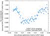 |
Fig. 5 Superposition of the transits of CoRoT-29b observed by CoRoT (small gray points) in 2011 and the transit observed by FTN in 2012 (large blue points). This is not a fit. In this figure we just superpose the FTN and the CoRoT data corrected from the contamination measured in the light curve. The contamination value was obtained exclusively from the fit to the CoRoT data. See text for discussion. |
Further ON-OFF photometry undertaken by the 3.5 m CFHT on 10 May 2013 also showed an on-target transit with a depth of 1.4 ± 0.3%.
A full transit of CoRoT-29b was observed with IAC80 in the night of 14 July 2014. The transit centre time, at BJD 2 456 853.435 ± 0.005, was used to refine the ephemeris in Table 6. It also shows some degree of asymmetry, though it is difficult to assess it with the same confidence level as for FTN data (see Fig. 6). The ingress is partially missing, complicating the assessment of any possible out-of-transit slope, either caused by stellar activity or by residuals of the data reduction (airmass correction, instrumentals, etc.).
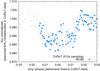 |
Fig. 6 Superposition of the transits of CoRoT-29b observed by CoRoT (small gray points) in 2011 and the transit observed by IAC80 in 2014 (large blue points). Same conditions as in Fig. 5. |
3.2. Radial velocity measurements
CoRoT-28b
Radial velocity measurements were first obtained with the SOPHIE (Perruchot et al. 2008; Bouchy et al. 2009) spectrograph on the 193 cm telescope at the Observatoire de Haute-Provence (France) and showed variations in phase with the CoRoT ephemeris, establishing the planetary nature of the candidate. A total of 25 radial velocity measurements were acquired in High Efficiency mode (R = 40 000) with SOPHIE between 27 August 2011 and 17 August 2012. An additional seven measurements between 7 July 2012 and 10 August 2013 were performed using the HARPS spectrograph in standard HAM mode (R = 115 000) (Mayor et al. 2003) mounted on the 3.6 m ESO telescope at La Silla Observatory (Chile) as part of the ESO large program 188.C-0779. Finally, ten spectra of CoRoT-28 were taken at different epochs between June and July 2012 using the FIbre-fed Échelle Spectrograph (FIES; Frandsen & Lindberg 1999; Telting et al. 2014) mounted at the 2.56-m Nordic Optical Telescope (NOT) of Roque de los Muchachos Observatory (La Palma, Spain). We employed the high-res fibre, which provides a resolving power of R = 67 000 in the spectral range 3600–7400 Å.
The SOPHIE and HARPS spectra were extracted using the respective pipelines. The radial velocities were then computed following a technique of weighted cross-correlation of the spectra using a numerical G2 star mask. This technique is described by Baranne et al. (1996) and Pepe et al. (2002). The spectral orders with low signal-to-noise ratio (S/N) were discarded to perform the computation to reduce the dispersion of the measurements. We eliminated the two bluest and five reddest orders for SOPHIE (39 in total), the ten bluest and the two reddest for HARPS (72 in total). The cross-correlation function of CoRoT-28b shows a single peak with FWHM of 9.9 km s-1 with SOPHIE and 7.6 km s-1 with HARPS. Also, SOPHIE and HARPS radial velocities obtained with different numerical spectral masks (F0, G2 and K5) show the same behaviour, suggesting that the radial velocity variations cannot be explained by a blend scenario with different spectral type stars.
For the FIES data, we adopted the same observing strategy described in Buchhave et al. (2010), i.e. we split each epoch observation into three consecutive exposures of 1200 s to remove cosmic rays hits, and we acquired long-exposed ThAr spectra in “sandwich-mode” to trace the RV drift of the instrument. We reduced the data using a customized IDL software suite, which includes bias subtraction, flat fielding, order tracing and extraction, and wavelength calibration. We obtained radial velocity measurements performing a multi-order cross-correlation with the RV standard star HD 182572, observed with the same instrument set-up as the target object, and for which we adopted an heliocentric radial velocity of − 100.350 km s-1, as measured by Udry et al. (1999).
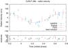 |
Fig. 7 Radial velocity measurements and best solution for CoRoT-28. Offsets have been subtracted according to the values given in Table 6. |
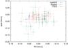 |
Fig. 8 Bisector span as a function of radial velocities for CoRoT-28. We subtracted the systemic velocities in the x axis. The uncertainties in the bisector span is assumed to be twice the uncertainties in the radial velocities. The bisector span shows no correlation with the radial velocities. |
The radial velocity measurements with the best orbital solution are shown in Fig. 7, assuming the period and transit epoch determined by the CoRoT light curve. Finally, the cross-correlation function bisector span shows no correlation with the radial velocities (see Fig. 8), reinforcing the conclusion that the radial velocity variations are not due to a blending effect. Radial velocities, their errors, and bisector span are listed in Tables A.1 to A.3.
For CoRoT-28b, we fit SOPHIE, HARPS, and FIES data together while fixing the ephemeris derived from the light-curve analysis (see Table 6). The rest of the orbital parameters (orbital eccentricity, argument of periastron, radial velocity semi-amplitude, and systemic velocities) were derived using the modelling procedure and Markov Chain Monte Carlo module from PASTIS (Díaz et al. 2014). The priors used for the orbital parameters were non-informative (uniform priors) except for the period and the transit epoch that were fixed. The results are summarized in Table 6.
CoRoT-29b
Because of its faintness (V = 15.6), CoRoT-29 radial velocity follow-up could only be performed with HARPS in the EGGS mode to improve the throughput. Compared to the HAM mode, which was used to follow up CoRoT-28, the EGGS mode of HARPS has a larger fiber (1.4″ compared to 1″) and no scrambler. The spectral resolution is therefore reduced (R = 80 000) but the throughput is twice as large. We obtained 20 measurements between 19 June 2012 and 10 August 2013, showing that the radial velocity variations were in agreement with the CoRoT ephemeris and establishing the planetary nature of CoRoT-29b (see Fig. 9). The same cross-correlation technique with a G2 spectral type numerical mask allowed us to derive the radial velocities. As for CoRoT-28, the ten bluest and the two reddest orders were discarded. We obtained a 7.1 km s-1 single peak cross-correlation function. Also, cross-correlation with other masks (F0 and K5) show no discrepancies in the radial velocity variations. Moreover, the cross-correlation function bisector span shows no correlation with the radial velocities (see Fig. 10). This suggests that the probability to have a blending effect is very low. The radial velocity measurements are represented in Fig. 9 and are listed with their errors and bisector spans in Table A.4.
We also fit CoRoT-29b HARPS data while fixing the ephemeris as described above for CoRoT-28b and the results are also summarized in Table 6.
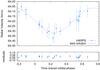 |
Fig. 9 Radial velocity measurements and best solution for CoRoT-29. Offsets were subtracted according to the values given in Table 6. |
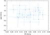 |
Fig. 10 Bisector span as a function of radial velocities for CoRoT-29. We subtracted the systemic velocities in the x axis. The uncertainties in the bisector span is assumed to be twice the uncertainties in the radial velocities. The bisector span shows no correlation with the radial velocities. |
3.3. Spectroscopic characterization
To derive the stellar parameters from the spectroscopic data, we used the Spectroscopy Made Easy (SME) package (version 5, February 2014). The development and structure and performance of SME is described in Valenti & Piskunov (1996) and in e.g. Valenti & Fischer (2005). Briefly, this code uses a grid of stellar models to which is fitted the observed spectrum. This is done by calculating a synthetized spectrum and minimizing the discrepancies through a non-linear, least-squares algorithm. The analysis is based on the latest generation of MARCS model atmospheres (Gustafsson et al. 2008) and the ATLAS12 models (Kurucz 2005). The models calculate the temperature and pressure distribution in radiative and hydrostatic equilibrium, assuming a plane-parallel stellar atmosphere.
Parameters of the fit to the transit light curve of CoRoT-28b.
The SME is developed so that, by matching synthetic spectra to observed line profiles, one can extract the information in the observed spectrum and search among stellar and atomic parameters until the best fit is achieved. The SME utilizes automatic parameter optimization using a Levenberg-Marquardt χ2 minimization algorithm. Synthetic spectra are calculated on the fly, by a built-in spectrum synthesis code, for a set of global model parameters and specified spectral line data. Starting from user-provided initial values, synthetic spectra are computed for small offsets in different directions for a subset of parameters defined to be “free”. The model atmospheres required for this are calculated through interpolating the grid of models mentioned above.
We used as input data the high-resolution spectra taken with HARPS (see Sect. 3.2). In the observed spectra ,we use a large number of spectral lines, e.g. the Balmer lines (the extended wings are used to constrain Teff), Na i D lines, Mg i b, and Ca i (for Teff and log g) and a large number of metal lines (to constrain the abundances). For CoRoT-28, we obtained a Li i equivalent width of 31 mÅ at 6708 Å.
After finding the Teff from the Balmer line wings (e.g. Fuhrmann et al. 1998), we use the calibration of Bruntt et al. (2010) to fix the micro- and macro-turbulence parameters before finding other parameters. The quoted errors are 1σ standard deviation errors in SME and thus a measure of how well the generation of the synthetic spectrum has succeeded. We know (Fridlund et al., in prep.) that when we apply SME to our (only) known source, the Sun, we find somewhat larger errors such as a ±100 K difference in Teff, and a ± 0.1dex in [Fe/H] (as proxy for metallicity) depending on the choice of model grid being used (e.g. Atlas12 or MARCS 2012). The mass, radius, and age of the star are calculated using stellar evolution tracks from Hurley et al. (2000) and the constraints from the analysis of the light curve (see Sect. 4). They are reported in Table 6.
Additionally, we estimated the interstellar extinction Av and spectroscopic distance d to CoRoT-28 and CoRoT-29 following the method described in Gandolfi et al. (2008). We simultaneously fitted the available ExoDat, 2MASS, and WISE colours (Table 1) with synthetic theoretical magnitudes derived by NextGen low-resolution model spectra (Hauschildt et al. 1999) having the same photospheric parameters as the stars. We excluded the W3 and W4 WISE magnitudes because of the low S/N. Assuming a normal extinction (Rv = 3.1), we found that CoRoT-28 and CoRoT-29 are at 560 ± 70 pc and 765 ± 50 pc from the Sun, and suffer an interstellar extinction of Av = 0.75 ± 0.20 mag and Av = 0.85 ± 0.15 mag, respectively. The dereddened B − V excess of the stars is 0.98 ± 0.06 and 0.87 ± 0.03 mag, respectively.
3.4. Spectral typing
A spectral type was derived for CoRoT-28 from a spectrum taken on 24 July 2012, with the
low-resolution spectrograph ( ) at the Nasmyth focus of the 2m telescope
in Tautenburg. A slit width of 1′′ and the V200 grism were used covering the wavelength range 360–935
nm. The S/N of the spectrum is about 180. The spectrum was reduced and extracted with IRAF
(Tody 1986, 1993) in the standard way, including subtraction of the bias and the background
as well as flat-field and extinction correction. Wavelengths were calibrated using sky
lines in the long-slit spectra and exposures of He and Kr gas discharge lamps. The
spectral type of CoRoT-28 was obtained following Gandolfi
et al. (2008) and Sebastian et al. (2012).
Briefly, we fitted the observed low-resolution spectrum using template spectra from the
library by Valdes et al. (2004) in combination with
the photospheric parameters derived by Wu et al.
(2011). Although a best match was attained for G8/G9V templates, we also found
matching templates with spectral classes G5-K0 and luminosity classes IV and III. The
luminosity class is not well defined by the low-resolution spectrum. For the reasons
explained above and considering the transit parameters, we consider that the star is
slightly evolved and classify it as G8/9IV. For CoRoT-29, considering the effective
temperature, we choose a spectral type K0V following Kenyon & Hartmann (1995).
) at the Nasmyth focus of the 2m telescope
in Tautenburg. A slit width of 1′′ and the V200 grism were used covering the wavelength range 360–935
nm. The S/N of the spectrum is about 180. The spectrum was reduced and extracted with IRAF
(Tody 1986, 1993) in the standard way, including subtraction of the bias and the background
as well as flat-field and extinction correction. Wavelengths were calibrated using sky
lines in the long-slit spectra and exposures of He and Kr gas discharge lamps. The
spectral type of CoRoT-28 was obtained following Gandolfi
et al. (2008) and Sebastian et al. (2012).
Briefly, we fitted the observed low-resolution spectrum using template spectra from the
library by Valdes et al. (2004) in combination with
the photospheric parameters derived by Wu et al.
(2011). Although a best match was attained for G8/G9V templates, we also found
matching templates with spectral classes G5-K0 and luminosity classes IV and III. The
luminosity class is not well defined by the low-resolution spectrum. For the reasons
explained above and considering the transit parameters, we consider that the star is
slightly evolved and classify it as G8/9IV. For CoRoT-29, considering the effective
temperature, we choose a spectral type K0V following Kenyon & Hartmann (1995).
4. Planetary parameters
4.1. CoRoT-28b
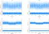 |
Fig. 11 The folded light curve of CoRoT-28b together with the best fit in the different chromatic light curves observed by CoRoT. Blue points are the observed data; the orange curves represent the individual fits. |
For the transit analysis and final planetary parameter determination of CoRoT-28b, we used the light curve that was filtered for stellar variability, as explained in Sect. 2.2, and the information from the spectral analysis described in Sect. 3. Since no significant transit timing variations (TTVs) were found, we folded the light curve using the ephemeris in Table 6. The folded light curve was then modelled with the Transit Light Curve Model code, described in Csizmadia et al. (2011). Each chromatic light curve (red, green, blue, and white, see Sect. 2.1) was treated in the same way. For the transit light-curve fit, we used the Mandel & Agol (2002) model. The optimization process consists of two steps. First, the best solution is found with a Harmony Search analysis genetic algorithm (Geem et al. 2001). Second, the uncertainties of the parameters are obtained via simulated annealing around the best solution found by the genetic algorithm.
The free parameters are the scaled semi-major axis (a/Rs, where
a is the
semi-major axis and Rs is the stellar radius), the
planet-to-stellar radius ratio (k =
Rp/Rs,
Rp is the planetary radius), the impact
parameter b,
where 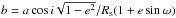 , i is the inclination,
e is the
eccentricity, and ω is the argument of the periastron. Values of
e and
ω are known
from the radial velocity analysis, and their uncertainties were propagated allowing them
to vary between their ±
1σ uncertainties during the optimization procedure.
The epoch could also vary within the uncertainties reported in Table 6. Following Csizmadia
et al. (2013), limb darkening coefficients were fitted as free parameters. We
took the results of Brown et al. (2001) and Pál & Kocsis (2008) into account, fitting the
combinations u+ =
ua +
ub and u− =
ua −
ub rather than the
linear and quadratic coefficients of ua and ub individually. A
quadratic limb darkening law provided a reasonable fit to the data.
, i is the inclination,
e is the
eccentricity, and ω is the argument of the periastron. Values of
e and
ω are known
from the radial velocity analysis, and their uncertainties were propagated allowing them
to vary between their ±
1σ uncertainties during the optimization procedure.
The epoch could also vary within the uncertainties reported in Table 6. Following Csizmadia
et al. (2013), limb darkening coefficients were fitted as free parameters. We
took the results of Brown et al. (2001) and Pál & Kocsis (2008) into account, fitting the
combinations u+ =
ua +
ub and u− =
ua −
ub rather than the
linear and quadratic coefficients of ua and ub individually. A
quadratic limb darkening law provided a reasonable fit to the data.
The fit is shown in Fig. 11 and the results can be seen in Table 2. The fits obtained in different colours are in agreement with each other. Note that because of the non-axisymmetric chromatic PSF of CoRoT, the contamination factors are not additive, so contamination in white is not equal to the sum of contaminations in different colours. The white light curve results were used to establish the planetary parameters given in Table 6 because they have the smallest uncertainties because of the higher S/N.
4.2. CoRoT-29b
As described in Sect. 2.3, the light curve of CoRoT-29b has a non-flat, mid-transit shape.
The CoRoT data sets sampled at 512 s and 32 s cadence were treated separately because of the background correction issue described in Sect. 2.4. The slope of the bottom part of the transit is non-zero with 95% confidence level in the 32 s sampled data by CoRoT, and only non-zero with 1σ significance in the 512 s sampled data set. It is also non-zero with 99% confidence level in the ground-based data from FTN, and non-zero with 95% confidence level in the IAC80 data (see Sect. 3.1). The slopes in the CoRoT data and in the ground-based data are compatible with each other within 1σ uncertainties, though the data from ground and from space were taken in slightly different wavelengths and suffer from different kind of systematic effects.
We have not been able to identify any systematic residual in the CoRoT data, which could account for the asymmetry of the transit; neither identified any other target in the CoRoT data set with a similar asymmetry. Ground-based observations are affected by correlated noise, which can produce asymmetries in the transit shape (see, for example, Hebb et al. 2010; Dittmann et al. 2010; Mancini et al. 2013). But in this case, despite the inherent limitations of the ground-based photometric observations that we present (see Sect. 3.1), we consider that the asymmetry observed by CoRoT is confirmed by the ground-based observations, and therefore it could have an astrophysical origin.
Possible interpretations for the asymmetry of the transit are given in the next Sect. 4.3, if the 2 sigma detection is assumed to be significant. The model that better reproduces the data is that including the gravity darkening produced by an oblate star (see Sect. 4.3.1). We have taken those values as the reference planetary parameters (see Table 6).
4.3. Interpretations of the transit light curve of CoRoT-29b
4.3.1. Stellar oblateness
We could interpret the shape of the light curve as the result of the transit of the
planet above a non-spherical stellar surface. A spherical surface becomes ellipsoidal,
in a first approximation, when it is deformed by its rotation, by its internal mass
distribution, or by the tidal influence of a massive companion. Consequently, the
stellar poles are closer to the centre of the star than the equator, thus the absorption
rate of photons from the stellar interior is different. Additionally, the effective
gravitational acceleration is higher at the poles than at the equator, where the
centrifugal force reaches its maximum. The decrease of the effective gravitational
acceleration at the equator affects the stellar atmospheric scale height, which in turn
changes the stellar temperature layering. All these effects cause a pole-to-equatorial
variation in the stellar flux, which is called gravity darkening, because this
temperature latitudinal variation is characterized by the effective surface gravity
g at a
certain latitude b and with a gravity darkening exponent
β,
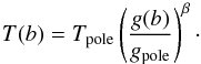 (1)The gravity darkening effect was studied by
von Zeipel (1924), Lucy (1967), Claret (1999,
2012) from theoretical point of view. In the
context of transiting extrasolar planets, this effect was studied in depth by Barnes (2009). Important observational results, in
eclipsing binary stars and transiting extrasolar planets, have been published by Rafert & Twigg (1980), Nakamura & Kitamura (1992), Djurašević et al. (2003), Szabó et al. (2011),
Morris et al. (2013), Barnes et al. (2013), Zhou & Huang (2013).
(1)The gravity darkening effect was studied by
von Zeipel (1924), Lucy (1967), Claret (1999,
2012) from theoretical point of view. In the
context of transiting extrasolar planets, this effect was studied in depth by Barnes (2009). Important observational results, in
eclipsing binary stars and transiting extrasolar planets, have been published by Rafert & Twigg (1980), Nakamura & Kitamura (1992), Djurašević et al. (2003), Szabó et al. (2011),
Morris et al. (2013), Barnes et al. (2013), Zhou & Huang (2013).
As is shown hereafter, we successfully explained the observed transit light-curve shape of CoRoT-29b with the assumption that the asymmetry of the light curve is caused by gravity darkening effect. We modelled this effect with our own code, which we briefly describe next, and which will be describe in detail in a future publication (Csizmadia, in prep.). The optimization method is identical to the one described before (see Sect. 4.1).
For this fit, we used the spectroscopic constraints for the v sin i and Teff from the spectroscopic analysis of the star. We allowed these parameters to vary between 3.5 ± 0.5 km s-1 and 5260 ± 70 K, respectively. Here Teff is the surface temperature of the star averaged for the visible hemisphere.
The stellar shape is defined by V = constant equipotential surfaces. We use the
quadrupolar approach (e.g. Zahn et al. 2010)
instead of the simple ellipsoidal approximation of Barnes
(2009), 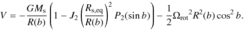 (2)This equation can be rewritten in a
dimensionless form as
(2)This equation can be rewritten in a
dimensionless form as 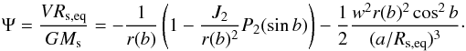 (3)Here we used the following notations:
-
Rs,eq, equatorial radius of the star,
-
G, gravitational constant,
-
Ms, mass of the star,
-
r(b) = R(b) /Rs,eq, the normalized radius of the star at latitude b,
-
w = Porb/Prot, a rotational parameter, namely the ratio of the orbital period of the planet and the rotational period of the star,
-
a/Rs,eq, the scaled semi-major axis where a is the semi-major axis of the planet,
-
J2, the second (or quadrupole’s) gravitational momentum of the star,
-
P2, the second Legendre-polynomial.
The free parameters are J2; the gravity darkening exponent
β; the
planet to stellar radius ratio k =
Rp/Rs; the
stellar inclination angle is (the obliquity of the star, as
defined in Barnes 2009, is ϕ = 90 −
is); Ωs, the sky projected angle of
the stellar spin axis (λ in the notation of Fabrycky & Winn 2009); ip, the inclination of the planetary
orbit; the limb darkening coefficients u+ and u−; the epoch
of the transit T0; the temperature of the star at the
pole Tpole; and the scaled semi-major axis
a/Rs,eq (see also
Figs. B.1 and 12). The rotational parameter w was calculated iteratively from the known
orbital period and from v sin i, assuming a certain average radius of the star.
We chose a stellar radius of 1 solar radius as initial value. After the first fit, we calculated
the density parameter  for the star. We searched stellar models
by Hurley et al. (2000), which provide this
density parameter at the effective surface temperature of the star (within the
uncertainties), and this yielded a new estimate for the stellar radius. With this new
stellar radius, we repeated the fit until convergence (see Fig. B.1).
for the star. We searched stellar models
by Hurley et al. (2000), which provide this
density parameter at the effective surface temperature of the star (within the
uncertainties), and this yielded a new estimate for the stellar radius. With this new
stellar radius, we repeated the fit until convergence (see Fig. B.1).
The stellar parameters define the value of Ψ. A Newton-Raphson iterative process yielded the value of r and the actual value of the surface gravity g = ∇V for every latitude and longitude. Then we calculated the effective surface temperature as well as the intensity assuming a simple black-body radiation for the star. A numerical integration procedure provided the unobscured flux of the star with a freely chosen gravity darkening exponent and limb darkening coefficients. As is well known, the limb darkening coefficients are functions of the effective stellar surface temperature. If the temperature varies over the surface, different limb darkening coefficients will be valid at each surface point. Since the theoretical limb darkening tables are not always in agreement with each other and they have not been validated observationally, it is hard to accept that an interpolation of these tables will provide the appropriate description of the limb darkening coefficients for every surface point. In addition, a rotating stellar atmosphere can be different from a static atmosphere, whereas most limb darkening tables use non-rotating stellar atmospheric models. Therefore, we left the limb darkening coefficients free and used a quadratic law hoping that this will be a better approximation of reality in this particular case. For further details about the difficulties of limb darkening handling, see Csizmadia et al. (2013). Our code also includes the rotational beaming effect.
Parameters of the fit to the transit light curve of CoRoT-29b with a model accounting for gravity darkening.
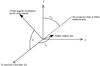 |
Fig. 12 Angle convention used in the gravity darkening model. |
The planet’s position was projected on the sky and when it crossed the apparent stellar disc, we calculated the amount of the blocked stellar emission in a small-planet approximation (Mandel & Agol 2002). Then we adjusted the free parameters until we had a convergence in the χ2-values, using the optimization methods described before (Sect. 4.1). The results of our modelling are shown in Table 3 and in graphical form in Fig. 13. The final planetary parameters are also shown in Table 6.
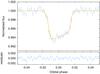 |
Fig. 13 Binned and folded light curve of CoRoT-29b together with the best fit accounting for gravity darkening fit. See text. |
4.3.2. Spherical star model
If we decide to ignore the non-flat shape of the transit and try to model the light curve of CoRoT-29b with the same techniques used in the case of CoRoT-28b (see Sect. 4.1), we obtain a fit solution significantly worse than using the more sophisticated analysis including gravitational darkening. The results are summarized in Table 4 and in graphical form in Fig. 14. Notice the remarkable distribution of the binned points relative to the fit. After the ingress, the observed points are systematically below the fit, and later, during the mid-eclipse and just before the egress phase they are systematically over the best match of the spherical star fit. We conclude that we cannot ignore the asymmetry of the light curve in the observed data set.
Parameters of the fit to the transit light curve of CoRoT-29b using a spherically symmetric model for the star.
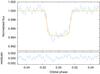 |
Fig. 14 Binned and folded light curve of CoRoT-29b together with the best fit using a spherically symmetric model of the star. We discarded this model as a correct explanation of the measured light curve as explained in the text. |
4.3.3. Spot-occulting model
Stellar spots occulted by transiting planets can have a significant impact in the measured transit light curve. This phenomenon has been widely studied in the literature and has been confirmed by several observations (Silva 2003; Wolter et al. 2009 and references therein; Sanchis-Ojeda et al. 2012, etc.). We require from a spot-occulting solution to reproduce the observed light curve with a stellar spot coverage, which is consistent with our knowledge of the stellar properties. Typically, the parameters used for this models are the stellar temperature and rotational period and the spot temperature, size, lifetime, and distribution.
In particular, the typical lifetime of a spot is ~2 weeks for the Sun, but other stars have both shorter and longer lifetimes, up to several months in some cases (Queloz et al. 2001). In our case, comparing the identical CoRoT and the FTN observations (see Sect. 3.1 and Fig. 5), we require a spot lifetime larger than one year.
Secondly, as all planetary transits observed by CoRoT in 2011 are indistinguishable with the current precision level, and they are also indistinguishable from FTN data from 2012 and IAC80 ground-based observations from 2014, we must conclude that the planet transits every 2.85 days above the same spot. This requires an exact synchronization between the stellar rotational period and the planetary orbital period, with exactly the same phase in a baseline larger than three years.
On the one hand, if the observed asymmetry is related to an equatorial or mid-latitude stellar spot, then the stellar rotational period should be equal to the orbital period of the planet, otherwise we cannot observe the spot always in phase with the planetary transits. However, we do not see a signature of such a spot as a modulation of the light curve in phase with the stellar rotational period. Moreover, we require the star to have a rotational period identical to the orbital period, which is not consistent with the stellar parameters derived from spectroscopy (in particular, with the v sin i).
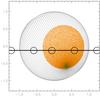 |
Fig. 15 Visualization of the CoRoT-29 system according to the spot model. The scale is in stellar radii. The orange area is the spotted area, while the horizontal line shows the sky-projected planetary orbit. The positions of the planet at different orbital phases are shown; the size of the circles correspond to the planetary radius in this scale. The pole of the star is denoted by a small green cross. |
On the other hand, if the spot is polar and the rotational axis of the star is perpendicular to the orbital plane of the planet, then we could not observe an asymmetric light curve. A spot-caused asymmetry requires an off-position of the spot from the apparent stellar disc. This scenario has the advantage that the signature of the spot is diluted in the light-curve signal, and we could not infer from the modulation of the light curve the stellar rotational period. Additionally, if the spot is centred on the pole and the stellar rotation axis has the right orientation, the planet could always cross the same location of the spotted region. This requires no prior assumptions on the stellar rotation period (see Fig. 15).
If we accept the polar spot scenario, however, which a priori cannot be ruled out as easily as the equatorial spot model, then we must require that the polar spot does not change its apparent position during the baseline of the observations. In this model, the rotational axis of the star is very different from the angular momentum of the vector of the planet, or in other words, the planetary orbit is misaligned with the equatorial plane of the star. The spot cannot be at the centre of the apparent stellar disc because of the asymmetry of the light curve. According to the light curve, the planet crosses the unspotted surface of the star first, producing a deeper transit, and later the spotted surface, when the lower brightness temperature of the spot produces a shallower transit. The apparent size of the spot should be much larger than the apparent size of the planet because we observe a continuous change in the transit depth and not a step-like event.
Polar spots in active stars are a common phenomenon and in some cases they can survive for long intervals of time. Or at least, active regions continuously producing spots at similar latitudes have been observed for several years in some young active stars like V410 Tau (Hatzes 1995; Rice et al. 2011). But these polar spots are on very active, young stars that are rapidly rotating (V410 Tau has a v sin i of 75 km s-1). Long-lived polar spots have never been seen, to our knowledge, on more slowly rotating stars like CoRoT-29. Moreover, these spots should produce signatures on the stellar spectrum (Ca ii emission, distortion in the line profiles, flat-bottomed line profiles), which are not observed in our data set (see Sect. 3).
Although it is unlikely that a spot can survive for such a long period without evolving on the surface of a main-sequence star, we used this assumption in our modelling with a spherical star, a spherical planet, and a circular spot on the surface of the star, with an arbitrarily oriented stellar rotational axis and arbitrary initial spot properties. We use a quadratic limb darkening law, as before. The results are given in Table 5 and shown in graphical form in Fig. 16.
Parameters of the fit to the transit light curve of CoRoT-29b using a spherically symmetric model for the star and a stellar spot.
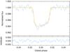 |
Fig. 16 Binned and folded light curve of CoRoT-29b together with the red line being the best fit using a spherically symmetric model for the star and a stellar spot. For comparison, the solid green curve is because of the unspotted light curve model (we set Tspot = Ts in the fitting routine). We discarded this model as a correct explanation of the measured light curve, as explained in the text. |
We obtain a polar spot with a tilted stellar rotational axis. This tilt means here that the projected rotational axis of the star and the projected angular momentum of the planet do not coincide. The planet is on “pole-on” orbit because it orbits the star in such a way that its projected orbit crosses the polar region of the star. The mutual inclination between the stellar equator and planetary orbital plane is practically 90 degrees. Note that such an orbit is very stable against perturbations.
From the measured v sin i and from the fitted stellar inclination for the spotted case (assuming Rs ~ 0.9 R⊙), we find that the stellar rotational period should be between 0.7–8.4 days. The spectroscopically measured v sin i ~ 3.5 km s-1 would yield veq ~ 10 km s-1 with is ≈ 20°, where the inclination of stellar rotational axis comes from the spot fit.
The comparison of the Bayesian Information Criterion (BIC) of the spot fit and the gravity darkening fit makes a clear choice which fit is better. The spot fit yielded BIC = 133, whereas the gravity darkening fit produces BIC = 120. This BIC difference corresponds to a Bayes factor of around 665 for the gravity darkening model (i.e. if the prior probabilities for each model are the same, then the gravity darkening is 665 times more probable than the spot model). Moreover, to explain the observational evidence we are obliged to put requirements on the size and temporal evolution of the spot, which are completely ad hoc. We consider that there is enough evidence to discard the spotted star as a reasonable interpretation of the data.
Planetary and stellar parameters.
An alternative to the single polar spot would be a band of spots with short lifetimes, but continuously appearing during the baseline of our observations in the same latitudes, relaxing one of the requirements of the scenario. One possibility is that if the spots were conveniently appearing at different longitudes, the condition of the synchronous rotation could also be relaxed. Including more spots will improve the modelling results at the cost of increasing the number of free parameters. Although plausible, it is finally also an ad hoc solution for the problem. This hypothesis could be falsified, however, if observations of the Rossiter–McLaughlin effect would show a small spin-orbit angle.
4.3.4. Planetary oblateness
A possible wind-driven oblated shaped of the planet can cause asymmetries in the light curve, but the observable amplitude is about 100 ppm (Barnes et al. 2009; Zhu et al. 2014), which is about 200 times smaller than the observed effect in our case, therefore we reject this explanation.
Other examples of star-planet interaction do not provide satisfactory answers in our case because they have typically different amplitudes and timescales (i.e. Jackson et al. 2012; Esteves et al. 2013; Faigler & Mazeh 2015).
4.3.5. Other scenarios
A disc around the star could produce an asymmetric transit, but there are no signs of such disc in the light curve or in the infrared emission of the star. A moon around the planet could produce an asymmetric transit, but dynamically there is no room for a moon around a planet so close to its star. A second planet in the system transiting simultaneously could produce an asymmetric transit, but not every time that the transit is observed, and there are no signs of this planet in the radial velocity. We conclude that none of these scenarios provides a satisfactory explanation of the data.
5. Discussion
5.1. Stellar properties
CoRoT-28
CoRoT-28 is a G8/9IV evolved star with a radius of approximately 1.8 solar radii. With an age of approximately 12 Gyr, we expect from gyrochronology a rotational period around 70 or 80 days and a v sin i around 1.2 km s-1 or smaller (Barnes 2007). The v sin i value from spectroscopy is almost three times larger, giving an expected rotational period of about 30 days. The autocorrelation function (ACF) of the light curve (see McQuillan et al. 2013) does not show any evident periodicity at all, but if there is any sign, it is for periods larger than the 85 days observed by CoRoT (see Fig. 17).
There is an inconsistency between the v sin i determined by spectroscopy, which is consistent with a relatively fast rotational period, and the stellar parameters derived from the models, which suggest an old star with a slow rotation rate. From our analysis of the light curve we cannot decide between the two scenarios. The v sin i has a relatively large uncertainty, but seems to be consistent with the higher rotation rate. It is possible that the stellar models fail to reproduce the actual age of the star. The range proposed by the models is 12.0 ± 1.5 Gyr, close to the old end of the distribution of stellar populations, which is consistent with the evolved stellar radius from the models (1.78 ± 0.11Rs for an effective temperature of 5150 ± 100 K). This range, however, is perhaps not as consistent with the metallicity [ Fe/H ] = 0.15 ± 0.05 dex, which is quite a robust observational result.
There is also an apparent inconsistency between the age and the Li i abundance in the atmosphere of the star. We estimated log N(Li) using Table 2 of Soderblom et al. (1993) given the equivalent width of 31 mÅ. For a dwarf with an effective temperature of 5150 K, we obtained log N(Li) = 1.4. This is in line with an age of a few hundred Myrs according to Sestito & Randich (2005). However, stars of this effective temperature with ages of few hundred Myrs have already reached the main sequence, which is not compatible with the surface gravity measured from spectroscopy or with the transit duration, which indicates that the star has a radius larger than the Sun. Moreover, we would expect a significant degree of stellar variability and a faster rotation period, which is also not supported by the observations. The abundance of lithium and its relationship with age, especially for stars hosting planets (see, for example, the recent discussions by Liu et al. 2014; Adamów et al. 2012), is still debated. Therefore we do not consider lithium as a reliable age indicator for CoRoT-28. On the other hand, it is known that a small amount of Li i can also be present in evolved stars, for example lithium can be regenerated by the Cameron-Fowler mechanism (Cameron & Fowler 1971).
We consider that observational evidence speaks in the case of CoRoT-28 in favour of an evolved star with a higher lithium content and v sin i value than what would be expected for its age and evolutionary status.
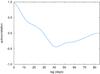 |
Fig. 17 Autocorrelation function of the light curve of CoRoT-28. |
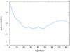 |
Fig. 18 Autocorrelation function of the light curve of CoRoT-29. |
CoRoT-29
CoRoT-29 is a K0 main-sequence star with a radius of approximately 0.9 solar radii. Its age is not well constrained from the analysis of the stellar models and the autocorrelation function of the light curve (see Fig. 18) does not help to constrain the rotational period. In any case, the analysis of the ACF in the case of CoRoT-29 can be debated, as ~50% of the flux within the mask comes from a contaminant.
It is however interesting that the analysis of the light curve (Sect. 4.3) shows that the orbital plane of the planet could be misaligned with respect to the equatorial plane of the star. The gravity darkening model allows us to measure the relative inclination of the spin axis of the star, a parameter that typically cannot be constrained with photometric measurements.
The alignment between the vector normal to the planetary orbital plane and the stellar spin axis is considered one of the key observables constraining planetary formation and evolution (for a recent discussion, see Dawson 2014, and references therein). It has been proposed that the alignment, or misalignment, is related to the dynamical interaction between the star and the planet, which in turn depends on the internal distribution of matter inside the star. Cold, convective stars have different dissipation timescales than hot, radiative stars (see Albrecht et al. 2012). CoRoT-29 with a Teff of 5260 K and with a misalignment angle4 of Ωs = 301 ± 30° would be right between the outliers of the distribution HAT-P-11 and HD 80606 in Fig. 20 of Albrecht et al. (2012). It is however worth mentioning that the tidal dissipation timescale of CoRoT-29b is 1000 times faster than for HAT-P-11, using Eq. (2) from the same paper. As mentioned, the dissipation timescale strongly depends on the internal structure of the star, which deserves further attention in the case of CoRoT-29.
The shape of the transit light curve of CoRoT-29b has a strong contribution from the gravity darkening, orders of magnitude larger than in other examples found (i.e. Szabó et al. 2011; Zhou & Huang 2013). The contributions are only comparable in the case of the pre-main-sequence star PTFO 8-8695 (Barnes et al. 2013). However, the origin of the gravity darkening effect in PTFO 8-8695 is the fast rotation of the star, a M dwarf with a radius of 1.4 R⊙, a rotational period of 10 h, and a v sin i of 80 km s-1. For CoRoT-29b, the origin of the extreme pole to equatorial radius difference is not as easily understood (see Fig. 19). The spectroscopically measured v sin i and the resulted stellar inclination (43°) yield veq = 5.1 ± 1.8 km s-1 and that corresponds to a stellar rotational period of 4–13 days.
 |
Fig. 19 Shape of the stellar surface of CoRoT-29 in the gravity darkening model (thick line) compared with a spherically symmetric star (thin line). |
To lowest order, and in the assumption of uniform rotation, the stellar shape is defined
by the surface of constant total potential as defined in Eq. (2). It shows the balance between the
contribution to the local gravitational potential of the stellar rotation Ωrot and the quadrupole moment
term dominated by J2. Actually, we should have included in
the balance the contribution from the tidal distortion caused by the planet, and account
for the misalignment between the rotation axis of the star and the angular momentum of the
orbit. But when comparing the tidal and rotational contributions to the distortion (see
Eq. (3) of Ragozzine & Wolf 2009 or A.21 of
Leconte et al. 2011), it turns out to be a couple
orders of magnitude less important, and so we neglect it. Note also that in Eq. (2) the contribution from rotation is negligible
compared to the contribution of the J2 term. This means that in our
modelling the rotation rate is constrained mainly by the v sin i value. The model can
measure the deformation and the orientation of the star, but not its rotation rate. The
results of Sect. 4.2 show that for CoRoT-29, the
quadrupole moment has a contribution 2 orders of magnitude larger than rotation. Actually,
the quadrupole moment of CoRoT-29 measured from the gravity darkening is far too large,
J2 = 0.028 ±
0.019, compared to the Sun,  (Lang
1999). Other authors have claimed large J2 values for
fast-rotating stars, such as WASP-33 (J2 = 3.8 × 10⁻⁴, Iorio 2011), but not as large as for CoRoT-29.
(Lang
1999). Other authors have claimed large J2 values for
fast-rotating stars, such as WASP-33 (J2 = 3.8 × 10⁻⁴, Iorio 2011), but not as large as for CoRoT-29.
The value of the quadrupolar moment depends on the distribution of matter inside the star. When the star is in uniform rotation, this quadrupolar moment is closely related to the Love number5k2 in the linear approximation. Indeed, once k2 is known, the external potential and the shape that a body exhibits in response to any perturbing potential can be computed (see, for example, Leconte et al. 2011). The Love number is a measure for the level of central condensation of an object: k2 decreases as the degree of central condensation increases. A homogeneous incompressible ideal fluid body has k2 = 3 / 2. For a star like CoRoT-29, the value of k2 can be estimated from canonical stellar models (see, for example, Claret & Gimenez 1995). Considering the v sin i value and the mass and orbital distance of the companion, the expected value of k2 for CoRoT-29 would produce a modest distortion, resulting in a J2 that would be 3 to 4 orders of magnitude smaller than our estimated value. In other words, the star is not rotating fast enough and the planetary companion is neither massive enough nor close enough to significantly distort the stellar shape. However, it is expected that the flattening may assume high values when the star is rotating differentially, with the angular velocity decreasing outwards (Jackson et al. 2004; Zahn et al. 2010). In turn, in the assumption of shellular rotation, a stellar rotation regime where the angular velocity is constant on level surfaces but varying in depth, (Zahn et al. 2010) has shown that J2 also increases compared to the case of uniform rotation. Assuming an internal differential rotation with a centre-to-surface ratio of 4 in angular velocity, the J2 of a 7 M⊙ rapidly rotating star like Archenar can exceed 0.01, which is about twice the value it assumes under the hypothesis of uniform rotation. It is not straightforward to infer how such a result could be extrapolated to a much less massive star and with slow surface rotation such as CoRoT-29. The star seems to be distorted and it is apparently a robust result, observed from space and independently confirmed from ground. The gravity darkening model provides the most accurate and reasonable explanation, although a dedicated modelling out of the scope of this paper would be required.
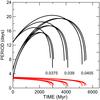 |
Fig. 20 Evolution of the period of rotation of the star in days. The red curve is the orbital period of the hypothetical falling planet. Initial semi-major axis as indicated. Initial eccentricity: e = 0.10. Initial rotation periods: 2, 5, and 12.8 days. |
5.2. Star-planet interaction
In the previous section, we have mentioned that the stars seem to rotate faster than expected for their evolutionary stage. In the case of CoRoT-29, for example, if magnetic braking is acting in this K0V star, and it is expected to be, the rotation should be slower. So, either the system is very young, or we have to find a mechanism to speed up the stellar rotation One way to speed up rotation is tidal interaction between the star and the planet. But the planets CoRoT-28b and CoRoT-29b may not be very efficient for that reason because of their orbital properties and, in the case of CoRoT-29b, for the high inclination of its orbit over the stellar equator (for a review of star-planet interaction in the CoRoT context, see Pätzold et al. 2012).
One hypothesis is that a second planet was present that accelerated the stellar rotation before falling into the star. Under this assumption, two planets formed simultaneously far away from the star (from the current position of the transiting planet). Planet-planet scattering could have moved then one planet in an inner orbit, very close to the star, and an outer planet in a larger, eccentric orbit. Tidal interactions would have made the inner planet fall into the star, accelerating its rotation rate and enriching its atmosphere with heavier elements such as lithium, while the outer planet would have subsequently circularized its orbit until the conditions that we see today.
To assess the viability of this kind of a scenario, we investigated the behaviour of such a hypothetical planet in the neighbourhood of the star. Although it is impossible to find observational evidence for this former planet, it is still useful to explore plausible mechanisms that can explain the current properties of CoRoT-29.
To reduce the number of free parameters, we assumed that the planet was a twin of CoRoT-29b in a low-eccentricity orbit. Figure 20 shows the evolution of the orbit of such a planet and the rotation of the star under the joint action of the magnetic braking of the star and the tides on the star caused by the planet. Regardless of the initial rotational rate of the star, all simulations show that the stellar rotation quickly increases to 15 to 20 days. At the same time, the semi-major axis of the planet is decreasing. At some point the tidal torque of the planet on the star becomes important and this accelerates the stellar rotation rate. By the time the planet has collided with the star, the rotational period has been reduced to a few days. After the collision, the stellar rotation rate brakes to its present value.
The models used in the evolution simulations are magnetic braking as determined by Bouvier et al. (1997) for stars with masses between 0.5 and 1.1 M⊙ and a creep tide (Ferraz-Mello 2013) due to a relaxation factor γ = 10 s-1. This choice corresponds to the mid of the tidal dissipation range determined from the statistical study of stars hosting hot Jupiters by Hansen (2010) (3–25 s-1; see Ferraz-Mello 2013). The great remaining difficulty is to discover how the existing planet CoRoT-29b could exist in same time as its falling sibling. The proximity of both orbits is prone to creating great instability; maybe the high inclination of CoRoT-29b is a consequence of this instability.
6. Summary
We have discovered and characterized two new planetary systems: CoRoT-28b and 29b.
CoRoT-28b belongs to the small population of hot-Jupiters orbiting evolved stars, which is interesting from the point of view of stellar and planetary evolution. It has a mass between that of Saturn and Jupiter and does not seem to be inflated (see the discussion in Enoch et al. 2012). There are a couple of open questions about the characterization of CoRoT-28, in particular regarding its rotation. We have measured a higher than expected v sin i and its lithium content is higher than expected for the star’s evolutionary status. These open questions might reveal important information about the past of the system. For example, there is the question of whether there was a former planet that fell into the star and thus accelerated the stellar rotation and enriched its atmosphere with heavy elements. Unfortunately, we cannot confirm this hypothesis because of the lack of observational evidence. We used the method described in Parviainen et al. (2013) to search for planet occultations (secondary eclipses) in the light curves, but we did not find any significant signal. For CoRoT-28b we obtain a maximum star-planet flux ratio of 9.5% (99th percentile of the marginal posterior). This upper limit is not useful for constraining the planet’s albedo or brightness temperature in any useful way, since the highest physically feasible value for f is ~2%.
CoRoT-29b is a very interesting system. The strong asymmetry of the transit light curve is only comparable to transits of planets orbiting very young, fast rotating stars, but the star is neither young nor rotating fast. The extreme value of the deformation, compared to stars of its mass range, is not understood and deserves more attention. We have not found at this point a satisfactory answer for the origin of the asymmetry in the transit shape, but we encourage the study of these system with other instruments (CHEOPS, Broeg et al. 2013; PLATO 2.0, Rauer et al. 2014, ground-based surveys) to confirm or disprove CoRoT observations and solve the puzzle.
Online material
Appendix A: Radial velocity data
CoRoT-28 SOPHIE radial velocities, their errors, and bisector spans.
CoRoT-28 HARPS radial velocities, their errors, and bisector spans.
CoRoT-28 FIES radial velocities, their errors, and bisector spans.
CoRoT-29 HARPS radial velocities, their errors, and bisector spans.
Appendix B: Flow chart for gravity darkening modelling
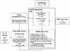 |
Fig. B.1 Flow chart for the gravity darkening modelling process of CoRoT-29b. |
For more information about the CoRoT data products, please see Baudin et al. (2006).
The version 3.0 of the data is already publicly accessible through the IAS CoRoT Archive (http://idoc-corot.ias.u-psud.fr/). The version 3.5 of the data will be publicly available in coming months.
Ωs is the sky projected angle of the stellar spin axis, λ in the notation of Fabrycky & Winn (2009). In the notation of Albrecht et al. (2012), it would be λ = 180 − Ωs.
Note that k2 is twice the apsidal motion constant, often indicated with the same symbol as in, e.g. Claret & Gimenez (1995).
Acknowledgments
We would like to thank the anonymous referee for comments, which led to substantial improvements of this paper. We are thankful for fruitful discussions to J.-P. Zahn (LUTh, Observatoire de Paris) and T. Borkovits (Baja Astronomical Observatory, Hungary). The team at LAM acknowledges support by CNES grants 98761 (SCCB), 251091 (JMA), and 426808 (CD). R.F.D. was supported by CNES via its postdoctoral fellowship program. A.S. acknowledges support from the European Research Council/European Community under the FP7 through Starting Grant agreement number 239953. A.S. is supported by the European Union under a Marie Curie Intra-European Fellowship for Career Development with reference FP7-PEOPLE-2013-IEF, number 627202. S.C.C.B. thanks CNES for the grant 98761. M.A. was supported by DLR (Deutsches Zentrum für Luft- und Raumfahrt) under the project 50 OW 0204. H.D. and P.K. acknowledge support by grant AYA2012-39346-C02-02 of the Spanish Secretary of State for R&D&i (MICINN). R.A. acknowledges the Spanish Ministry of Economy and Competitiveness (MINECO) for the financial support under the Ramón y Cajal program RYC-2010-06519, and by grant ESP2013-48391-C4-2-R. This research made use of data acquired with the IAC80 telescope, operated at Teide Observatory on the island of Tenerife by the Instituto de Astrofísica de Canarias. Some of the data presented were acquired with the Nordic Optical Telescope, operated by the Nordic Optical Telescope Scientific Association at the Observatorio del Roque de los Muchachos, La Palma, Spain, of the Instituto de Astrofísica de Canarias, under OPTICON programme 2012A033 and CAT programme 91-NOT7/12A. We would like to thank the workshops and the night assistants at the observatory in Tautenburg, Germany. We are thankful to A. Almazan for the observations taken for this paper. This research has made use of the ExoDat database, operated at LAM-OAMP, Marseille, France, on behalf of the CoRoT/Exoplanet program. This publication makes use of data products from the Two Micron All Sky Survey, which is a joint project of the University of Massachusetts and the Infrared Processing and Analysis Center/California Institute of Technology, funded by the National Aeronautics and Space Administration and the National Science Foundation. Funding for the Sloan Digital Sky Survey (SDSS) has been provided by the Alfred P. Sloan Foundation, the Participating Institutions, the National Aeronautics and Space Administration, the National Science Foundation, the US Department of Energy, the Japanese Monbukagakusho, and the Max Planck Society. The SDSS Web site is http://www.sdss.org/. This research has made use of NASA’s Astrophysics Data System.
References
- Adamów, M., Niedzielski, A., Villaver, E., Nowak, G., & Wolszczan, A. 2012, ApJ, 754, L15 [NASA ADS] [CrossRef] [Google Scholar]
- Alapini, A., & Aigrain, S. 2009, MNRAS, 397, 1591 [NASA ADS] [CrossRef] [Google Scholar]
- Albrecht, S., Winn, J. N., Johnson, J. A., et al. 2012, ApJ, 757, 18 [NASA ADS] [CrossRef] [Google Scholar]
- Auvergne, M., Bodin, P., Boisnard, L., et al. 2009, A&A, 506, 411 [NASA ADS] [CrossRef] [EDP Sciences] [Google Scholar]
- Baglin, A., Auvergne, M., Boisnard, L., et al. 2006, in COSPAR, Plenary Meeting, 36th COSPAR Scientific Assembly, 3749 [Google Scholar]
- Baranne, A., Queloz, D., Mayor, M., et al. 1996, A&AS, 119, 373 [NASA ADS] [CrossRef] [EDP Sciences] [Google Scholar]
- Barge, P., Baglin, A., Auvergne, M., & the CoRoT team. 2008, IAU Symp., 249, 3 [Google Scholar]
- Barnes, S. A. 2007, ApJ, 669, 1167 [NASA ADS] [CrossRef] [Google Scholar]
- Barnes, J. W. 2009, ApJ, 705, 683 [Google Scholar]
- Barnes, J. W., Cooper, C. S., Showman, A. P., & Hubbard, W. B. 2009, ApJ, 706, 877 [NASA ADS] [CrossRef] [Google Scholar]
- Barnes, J. W., van Eyken, J. C., Jackson, B. K., Ciardi, D. R., & Fortney, J. J. 2013, ApJ, 774, 53 [NASA ADS] [CrossRef] [Google Scholar]
- Baudin, F., Baglin, A., Orcesi, J.-L., et al. 2006, in ESA SP 1306, eds. M. Fridlund, A. Baglin, J. Lochard, & L. Conroy, 145 [Google Scholar]
- Boisnard, L., & Auvergne, M. 2006, in ESA SP 1306, eds. M. Fridlund, A. Baglin, J. Lochard, & L. Conroy, 19 [Google Scholar]
- Bonomo, A. S., Chabaud, P. Y., Deleuil, M., et al. 2012, A&A, 547, A110 [NASA ADS] [CrossRef] [EDP Sciences] [Google Scholar]
- Borucki, W. J., Koch, D., Basri, G., et al. 2010, Science, 327, 977 [NASA ADS] [CrossRef] [PubMed] [Google Scholar]
- Bouchy, F., Hébrard, G., Udry, S., et al. 2009, A&A, 505, 853 [NASA ADS] [CrossRef] [EDP Sciences] [Google Scholar]
- Bouvier, J., Forestini, M., & Allain, S. 1997, A&A, 326, 1023 [NASA ADS] [Google Scholar]
- Broeg, C., Fortier, A., Ehrenreich, D., et al. 2013, EPJ Web Conf., 47, 3005 [Google Scholar]
- Brown, T. M., Charbonneau, D., Gilliland, R. L., Noyes, R. W., & Burrows, A. 2001, ApJ, 552, 699 [NASA ADS] [CrossRef] [Google Scholar]
- Bruntt, H., Bedding, T. R., Quirion, P.-O., et al. 2010, MNRAS, 405, 1907 [NASA ADS] [Google Scholar]
- Buchhave, L. A., Bakos, G. Á., Hartman, J. D., et al. 2010, ApJ, 720, 1118 [NASA ADS] [CrossRef] [Google Scholar]
- Cameron, A. G. W., & Fowler, W. A. 1971, ApJ, 164, 111 [Google Scholar]
- Claret, A. 1999, in Stellar Structure: Theory and Test of Connective Energy Transport, eds. A. Gimenez, E. F. Guinan, & B. Montesinos, ASP Conf. Ser., 173, 277 [Google Scholar]
- Claret, A. 2012, A&A, 538, A3 [NASA ADS] [CrossRef] [EDP Sciences] [Google Scholar]
- Claret, A., & Gimenez, A. 1995, A&AS, 114, 549 [NASA ADS] [Google Scholar]
- Csizmadia, S., Moutou, C., Deleuil, M., et al. 2011, A&A, 531, A41 [NASA ADS] [CrossRef] [EDP Sciences] [Google Scholar]
- Csizmadia, S., Pasternacki, T., Dreyer, C., et al. 2013, A&A, 549, A9 [NASA ADS] [CrossRef] [EDP Sciences] [Google Scholar]
- Dawson, R. I. 2014, ApJ, 790, L31 [NASA ADS] [CrossRef] [Google Scholar]
- Deeg, H. J., Gillon, M., Shporer, A., et al. 2009, A&A, 506, 343 [NASA ADS] [CrossRef] [EDP Sciences] [Google Scholar]
- Deleuil, M., Meunier, J. C., Moutou, C., et al. 2009, AJ, 138, 649 [NASA ADS] [CrossRef] [Google Scholar]
- Díaz, R. F., Almenara, J. M., Santerne, A., et al. 2014, MNRAS, 441, 983 [NASA ADS] [CrossRef] [Google Scholar]
- Dittmann, J. A., Close, L. M., Scuderi, L. J., & Morris, M. D. 2010, ApJ, 717, 235 [NASA ADS] [CrossRef] [Google Scholar]
- Djurašević, G., Rovithis-Livaniou, H., Rovithis, P., et al. 2003, A&A, 402, 667 [NASA ADS] [CrossRef] [EDP Sciences] [Google Scholar]
- Enoch, B., Collier Cameron, A., & Horne, K. 2012, A&A, 540, A99 [NASA ADS] [CrossRef] [EDP Sciences] [Google Scholar]
- Esteves, L. J., De Mooij, E. J. W., & Jayawardhana, R. 2013, ApJ, 772, 51 [NASA ADS] [CrossRef] [Google Scholar]
- Fabrycky, D. C., & Winn, J. N. 2009, ApJ, 696, 1230 [NASA ADS] [CrossRef] [Google Scholar]
- Faigler, S., & Mazeh, T. 2015, ApJ, 800, 73 [NASA ADS] [CrossRef] [Google Scholar]
- Ferraz-Mello, S. 2013, Celest. Mech. Dyn. Astron., 116, 109 [NASA ADS] [CrossRef] [Google Scholar]
- Frandsen, S., & Lindberg, B. 1999, in Astrophysics with the NOT, eds. H. Karttunen, & V. Piirola, 71 [Google Scholar]
- Fuhrmann, K., Pfeiffer, M. J., & Bernkopf, J. 1998, A&A, 336, 942 [NASA ADS] [Google Scholar]
- Gandolfi, D., Alcalá, J. M., Leccia, S., et al. 2008, ApJ, 687, 1303 [NASA ADS] [CrossRef] [Google Scholar]
- Geem, Z. G., Kim, J. H., & Loganathan, G. V. 2001, Simulation, 76, 60 [CrossRef] [Google Scholar]
- Gustafsson, B., Edvardsson, B., Eriksson, K., et al. 2008, A&A, 486, 951 [NASA ADS] [CrossRef] [EDP Sciences] [Google Scholar]
- Hansen, B. M. S. 2010, ApJ, 723, 285 [NASA ADS] [CrossRef] [Google Scholar]
- Hatzes, A. P. 1995, ApJ, 451, 784 [NASA ADS] [CrossRef] [Google Scholar]
- Hauschildt, P. H., Allard, F., & Baron, E. 1999, ApJ, 512, 377 [NASA ADS] [CrossRef] [Google Scholar]
- Hebb, L., Collier-Cameron, A., Triaud, A. H. M. J., et al. 2010, ApJ, 708, 224 [NASA ADS] [CrossRef] [Google Scholar]
- Hurley, J. R., Pols, O. R., & Tout, C. A. 2000, MNRAS, 315, 543 [NASA ADS] [CrossRef] [Google Scholar]
- Iorio, L. 2011, Ap&SS, 331, 485 [NASA ADS] [CrossRef] [Google Scholar]
- Jackson, S., MacGregor, K. B., & Skumanich, A. 2004, ApJ, 606, 1196 [NASA ADS] [CrossRef] [Google Scholar]
- Jackson, B. K., Lewis, N. K., Barnes, J. W., et al. 2012, ApJ, 751, 112 [NASA ADS] [CrossRef] [Google Scholar]
- Kenyon, S. J., & Hartmann, L. 1995, ApJS, 101, 117 [NASA ADS] [CrossRef] [Google Scholar]
- Kurucz, R. L. 2005, Mem. Soc. Astron. It. Suppl., 8, 14 [Google Scholar]
- Lang, K. R. 1999, Astrophysical formulae (New York: Springer) [Google Scholar]
- Leconte, J., Lai, D., & Chabrier, G. 2011, A&A, 536, C1 [NASA ADS] [CrossRef] [EDP Sciences] [Google Scholar]
- Liu, Y. J., Tan, K. F., Wang, L., et al. 2014, ApJ, 785, 94 [NASA ADS] [CrossRef] [Google Scholar]
- Lucy, L. B. 1967, ZAp, 65, 89 [NASA ADS] [Google Scholar]
- Mancini, L., Southworth, J., Ciceri, S., et al. 2013, A&A, 551, A11 [NASA ADS] [CrossRef] [EDP Sciences] [Google Scholar]
- Mandel, K., & Agol, E. 2002, ApJ, 580, L171 [NASA ADS] [CrossRef] [Google Scholar]
- Mayor, M., Pepe, F., Queloz, D., et al. 2003, The Messenger, 114, 20 [NASA ADS] [Google Scholar]
- McQuillan, A., Aigrain, S., & Mazeh, T. 2013, MNRAS, 432, 1203 [NASA ADS] [CrossRef] [MathSciNet] [Google Scholar]
- Morris, B. M., Mandell, A. M., & Deming, D. 2013, ApJ, 764, L22 [NASA ADS] [CrossRef] [Google Scholar]
- Moutou, C., Pont, F., Bouchy, F., et al. 2009, A&A, 506, 321 [NASA ADS] [CrossRef] [EDP Sciences] [Google Scholar]
- Nakamura, Y., & Kitamura, M. 1992, Ap&SS, 191, 267 [NASA ADS] [CrossRef] [Google Scholar]
- Pál, A., & Kocsis, B. 2008, MNRAS, 389, 191 [NASA ADS] [CrossRef] [Google Scholar]
- Parviainen, H., Deeg, H. J., & Belmonte, J. A. 2013, A&A, 550, A67 [NASA ADS] [CrossRef] [EDP Sciences] [Google Scholar]
- Pätzold, M., Endl, M., Csizmadia, S., et al. 2012, A&A, 545, A6 [NASA ADS] [CrossRef] [EDP Sciences] [Google Scholar]
- Pepe, F., Mayor, M., Galland, F., et al. 2002, A&A, 388, 632 [NASA ADS] [CrossRef] [EDP Sciences] [Google Scholar]
- Perruchot, S., Kohler, D., Bouchy, F., et al. 2008, in SPIE Conf. Ser., 7014 [Google Scholar]
- Queloz, D., Henry, G. W., Sivan, J. P., et al. 2001, A&A, 379, 279 [NASA ADS] [CrossRef] [EDP Sciences] [Google Scholar]
- Rafert, J. B., & Twigg, L. W. 1980, MNRAS, 193, 79 [NASA ADS] [CrossRef] [Google Scholar]
- Ragozzine, D., & Wolf, A. S. 2009, ApJ, 698, 1778 [NASA ADS] [CrossRef] [Google Scholar]
- Rauer, H., Catala, C., Aerts, C., et al. 2014, Exper. Astron., 38, 249 [Google Scholar]
- Reid, I. N., Brewer, C., Brucato, R. J., et al. 1991, PASP, 103, 661 [NASA ADS] [CrossRef] [Google Scholar]
- Rice, J. B., Strassmeier, K. G., & Kopf, M. 2011, ApJ, 728, 69 [NASA ADS] [CrossRef] [Google Scholar]
- Sanchis-Ojeda, R., Fabrycky, D. C., Winn, J. N., et al. 2012, Nature, 487, 449 [NASA ADS] [CrossRef] [PubMed] [Google Scholar]
- Sebastian, D., Guenther, E. W., Schaffenroth, V., et al. 2012, A&A, 541, A34 [NASA ADS] [CrossRef] [EDP Sciences] [Google Scholar]
- Sestito, P., & Randich, S. 2005, A&A, 442, 615 [NASA ADS] [CrossRef] [EDP Sciences] [Google Scholar]
- Silva, A. V. R. 2003, ApJ, 585, L147 [NASA ADS] [CrossRef] [Google Scholar]
- Soderblom, D. R., Jones, B. F., Balachandran, S., et al. 1993, AJ, 106, 1059 [NASA ADS] [CrossRef] [Google Scholar]
- Szabó, G. M., Szabó, R., Benkő, J. M., et al. 2011, ApJ, 736, L4 [NASA ADS] [CrossRef] [Google Scholar]
- Telting, J. H., Avila, G., Buchhave, L., et al. 2014, Astron. Nachr., 335, 41 [NASA ADS] [CrossRef] [Google Scholar]
- Tody, D. 1986, in Instrumentation in astronomy VI, ed. D. L. Crawford, SPIE Conf. Ser., 627, 733 [Google Scholar]
- Tody, D. 1993, in Astronomical Data Analysis Software and Systems II, eds. R. J. Hanisch, R. J. V. Brissenden, & J. Barnes, ASP Conf. Ser., 52, 173 [Google Scholar]
- Udry, S., Mayor, M., & Queloz, D. 1999, in IAU Colloq. 170: Precise Stellar Radial Velocities, eds. J. B. Hearnshaw, & C. D. Scarfe, ASP Conf. Ser., 185, 367 [Google Scholar]
- Valdes, F., Gupta, R., Rose, J. A., Singh, H. P., & Bell, D. J. 2004, ApJS, 152, 251 [NASA ADS] [CrossRef] [Google Scholar]
- Valenti, J. A., & Fischer, D. A. 2005, ApJS, 159, 141 [NASA ADS] [CrossRef] [MathSciNet] [Google Scholar]
- Valenti, J. A., & Piskunov, N. 1996, A&AS, 118, 595 [NASA ADS] [CrossRef] [EDP Sciences] [Google Scholar]
- von Zeipel, H. 1924, MNRAS, 84, 665 [NASA ADS] [CrossRef] [Google Scholar]
- Wolter, U., Schmitt, J. H. M. M., Huber, K. F., et al. 2009, A&A, 504, 561 [NASA ADS] [CrossRef] [EDP Sciences] [Google Scholar]
- Wright, E. L., Eisenhardt, P. R. M., Mainzer, A. K., et al. 2010, AJ, 140, 1868 [NASA ADS] [CrossRef] [Google Scholar]
- Wu, Y., Luo, A.-L., Li, H.-N., et al. 2011, RA&A, 11, 924 [Google Scholar]
- Zahn, J.-P., Ranc, C., & Morel, P. 2010, A&A, 517, A7 [NASA ADS] [CrossRef] [EDP Sciences] [Google Scholar]
- Zhou, G., & Huang, C. X. 2013, ApJ, 776, L35 [NASA ADS] [CrossRef] [Google Scholar]
- Zhu, W., Huang, C. X., Zhou, G., & Lin, D. N. C. 2014, ApJ, 796, 67 [NASA ADS] [CrossRef] [Google Scholar]
All Tables
Parameters of the fit to the transit light curve of CoRoT-29b with a model accounting for gravity darkening.
Parameters of the fit to the transit light curve of CoRoT-29b using a spherically symmetric model for the star.
Parameters of the fit to the transit light curve of CoRoT-29b using a spherically symmetric model for the star and a stellar spot.
All Figures
|
Fig. 1 Second Palomar Observatory Sky Survey (POSS II, Reid et al. 1991) image around the CoRoT-28 (left) and CoRoT-29 (right) targets. We have over-plotted the CoRoT masks used in the observations and we give identification labels for the brightest, closest background stars. The mask of CoRoT-28 shows the subdivision in the three submasks, named from north to south: red, green, and blue. |
| In the text | |
|
Fig. 2 Raw light curve of CoRoT-28. The original data points, sampled at 32 s, are shown in blue. We have binned the data to 512 s bins to guide the eye. |
| In the text | |
|
Fig. 3 Iterative filtering applied to the light curve of CoRoT-29b, converging in three steps (labelled A, B, and C). Top of each panel shows the light curve (normalized flux vs. CoRoT Julian Date, which is HJD − 2 451 545.0), the bottom figures on each panel show the folded light curves (normalized flux vs. orbital phase). |
| In the text | |
|
Fig. 4 Change in the transit depth of CoRoT-29b observed in the light curves sampled at 512 s and 32 s (version 3.0 of the data). |
| In the text | |
|
Fig. 5 Superposition of the transits of CoRoT-29b observed by CoRoT (small gray points) in 2011 and the transit observed by FTN in 2012 (large blue points). This is not a fit. In this figure we just superpose the FTN and the CoRoT data corrected from the contamination measured in the light curve. The contamination value was obtained exclusively from the fit to the CoRoT data. See text for discussion. |
| In the text | |
|
Fig. 6 Superposition of the transits of CoRoT-29b observed by CoRoT (small gray points) in 2011 and the transit observed by IAC80 in 2014 (large blue points). Same conditions as in Fig. 5. |
| In the text | |
|
Fig. 7 Radial velocity measurements and best solution for CoRoT-28. Offsets have been subtracted according to the values given in Table 6. |
| In the text | |
|
Fig. 8 Bisector span as a function of radial velocities for CoRoT-28. We subtracted the systemic velocities in the x axis. The uncertainties in the bisector span is assumed to be twice the uncertainties in the radial velocities. The bisector span shows no correlation with the radial velocities. |
| In the text | |
|
Fig. 9 Radial velocity measurements and best solution for CoRoT-29. Offsets were subtracted according to the values given in Table 6. |
| In the text | |
|
Fig. 10 Bisector span as a function of radial velocities for CoRoT-29. We subtracted the systemic velocities in the x axis. The uncertainties in the bisector span is assumed to be twice the uncertainties in the radial velocities. The bisector span shows no correlation with the radial velocities. |
| In the text | |
|
Fig. 11 The folded light curve of CoRoT-28b together with the best fit in the different chromatic light curves observed by CoRoT. Blue points are the observed data; the orange curves represent the individual fits. |
| In the text | |
|
Fig. 12 Angle convention used in the gravity darkening model. |
| In the text | |
|
Fig. 13 Binned and folded light curve of CoRoT-29b together with the best fit accounting for gravity darkening fit. See text. |
| In the text | |
|
Fig. 14 Binned and folded light curve of CoRoT-29b together with the best fit using a spherically symmetric model of the star. We discarded this model as a correct explanation of the measured light curve as explained in the text. |
| In the text | |
|
Fig. 15 Visualization of the CoRoT-29 system according to the spot model. The scale is in stellar radii. The orange area is the spotted area, while the horizontal line shows the sky-projected planetary orbit. The positions of the planet at different orbital phases are shown; the size of the circles correspond to the planetary radius in this scale. The pole of the star is denoted by a small green cross. |
| In the text | |
|
Fig. 16 Binned and folded light curve of CoRoT-29b together with the red line being the best fit using a spherically symmetric model for the star and a stellar spot. For comparison, the solid green curve is because of the unspotted light curve model (we set Tspot = Ts in the fitting routine). We discarded this model as a correct explanation of the measured light curve, as explained in the text. |
| In the text | |
|
Fig. 17 Autocorrelation function of the light curve of CoRoT-28. |
| In the text | |
|
Fig. 18 Autocorrelation function of the light curve of CoRoT-29. |
| In the text | |
|
Fig. 19 Shape of the stellar surface of CoRoT-29 in the gravity darkening model (thick line) compared with a spherically symmetric star (thin line). |
| In the text | |
|
Fig. 20 Evolution of the period of rotation of the star in days. The red curve is the orbital period of the hypothetical falling planet. Initial semi-major axis as indicated. Initial eccentricity: e = 0.10. Initial rotation periods: 2, 5, and 12.8 days. |
| In the text | |
|
Fig. B.1 Flow chart for the gravity darkening modelling process of CoRoT-29b. |
| In the text | |
Current usage metrics show cumulative count of Article Views (full-text article views including HTML views, PDF and ePub downloads, according to the available data) and Abstracts Views on Vision4Press platform.
Data correspond to usage on the plateform after 2015. The current usage metrics is available 48-96 hours after online publication and is updated daily on week days.
Initial download of the metrics may take a while.