| Issue |
A&A
Volume 578, June 2015
|
|
|---|---|---|
| Article Number | A63 | |
| Number of page(s) | 16 | |
| Section | Numerical methods and codes | |
| DOI | https://doi.org/10.1051/0004-6361/201525740 | |
| Published online | 05 June 2015 | |
Interpreting observations of molecular outflow sources: the MHD shock code mhd_vode⋆
1 Physics Department, The University, Durham DH1 3LE, UK
e-mail: This email address is being protected from spambots. You need JavaScript enabled to view it.
2 IAS (UMR 8617 du CNRS), Bâtiment 121, Université de Paris Sud, 91405 Orsay, France
e-mail: This email address is being protected from spambots. You need JavaScript enabled to view it.
3 LERMA (UMR 8112 du CNRS), Observatoire de Paris, 61 avenue de l’Observatoire, 75014 Paris, France
Received: 26 January 2015
Accepted: 11 March 2015
Abstract
The planar MHD shock code mhd_vode has been developed in order to simulate both continuous (C) type shock waves and jump (J) type shock waves in the interstellar medium. The physical and chemical state of the gas in steady-state may also be computed and used as input to a shock wave model. The code is written principally in FORTRAN 90, although some routines remain in FORTRAN 77. The documented program and its input data are described and provided as supplementary material, and the results of exemplary test runs are presented. Our intention is to enable the interested user to run the code for any sensible parameter set and to comprehend the results. With applications to molecular outflow sources in mind, we have computed, and are making available as supplementary material, integrated atomic and molecular line intensities for grids of C- and J-type models; these computations are summarized in the Appendices.
Key words: astrochemistry / stars: formation / ISM: jets and outflows / ISM: kinematics and dynamics / infrared: ISM
Appendix tables, a copy of the current version of the code, and of the two model grids are only available at the CDS via anonymous ftp to cdsarc.u-strasbg.fr (130.79.128.5) or via http://cdsarc.u-strasbg.fr/viz-bin/qcat?J/A+A/578/A63
© ESO, 2015
1. Introduction
An earlier version of this MHD shock program was described by Heck et al. (1990). The code has been modified extensively since that time, with the principal astronomical motivation being to model the emission from shocks in the molecular outflows associated with low-mass star formation. The spectroscopic data acquired by satellites such as ISO, Herschel and Spitzer have provided the motivation for developing the code in order to predict the intensities of molecular lines in the sub-mm and the infrared.
The program solves a set of coupled, first-order ordinary differential equations by means of the DVODE algorithm, which is able to treat “stiff” differential equations. DVODE was developed by Hindmarsh (1983) and collaborators from the method described by Gear (1971). This method has proved reliable and robust and has been used to solve sets of up to 103 coupled equations. The shock code includes the requisite interface with the DVODE package; it calls routines in the BLAS and LAPACK libraries. The program is in modular form, with compilation being facilitated by means of a Makefile, where the FORTRAN compiler and the links to the libraries can be modified to suit the system requirements of the user. The program has been run successfully using gfortran and pgf90 (Portland Group) compilers, producing essentially identical results. Input data are read from the corresponding input folder and the numerical results are directed to the output folder.
The module mhd_vode.f90 contains the Main program, which controls the numerical integration of the coupled differential equations by calls to the DVODE package, integrateur_vode.f. The requisite derivatives of the dependent variables, yi, are evaluated in subroutine DIFFUN, to be found in evolution.f90. In practice, the logarithmic derivatives. d(lnyi) /dz, of the dependent variables, rather than the variables themselves, are integrated; the independent variable, z, is the distance from the starting point of the integration, which is located in the preshock gas, and is measured along the perpendicular to the (planar) shock front.
The flow time of the (neutral) fluid through the shock wave is related to the independent variable through the relation  where vn is the neutral flow speed. The numerical integration is terminated when a specified maximum flow time (duration_max) or number of integration steps (Nstep_max) has been reached.
The quantities to be integrated are the (multi-fluid) dynamical variables, the number densities of the chemical species, and the population densities of the specified energy levels of the molecules whose line intensities are computed, viz. ortho- and para-H2, CO, SiO, ortho- and para-H2O, ortho- and para-NH3, OH, and A- and E-type CH3OH (optional). DIFFUN sets up the differential equations, making calls to other routines that evaluate the source terms, which appear on the rhs of the differential equations. The source terms determine the net gain or loss of mass, number density, linear momentum, and energy of the neutral, positively and negatively charged fluids, the net creation or destruction of each of the chemical species, and the net gain or loss of population of a given molecular energy level. With the exception of H2, whose lines are optically thin, the molecular line opacities are evaluated in the large velocity gradient (LVG) approximation, which is well adapted to the conditions in shock waves. The reading and processing of the list of chemical species and the associated chemical reactions are controlled by the modules chemical_species.f90 and chemical_reactions.f90, respectively. The molecular line transfer and radiative cooling are treated in a series of modules, CO.f, OH.f, oH2O.f, oNH3.f, pH2O.f, pNH3.f, SiO.f, and Atype.f, Etype.f; the corresponding calculations for H2 are performed in H2.f90. The module molecular_cooling.f90 contains an earlier and more approximate treatment of the molecular cooling and is largely redundant; it is retained in case the user wishes to render the computations faster by sacrificing the higher precision afforded by the LVG approximation.
The calculations may be performed without the LVG treatment of radiation transfer in the lines of methanol, which may not always be of interest; this mode of operation requires significantly less computer time, owing the reduction in the number of coupled differential equations that have to be integrated. Much faster still is the option of eliminating completely the LVG method and using more approximate treatments of the rates of cooling by the principal molecules. In this case, a complete model can be run in minutes, rather than hours, on a typical modern processor.
In addition to the intensities of molecular emission lines, the program computes the following atomic and ionic forbidden line spectra: [C I], [C II], [N I], [N II], [O I], [O II], [Si I], [Si II], [S I], [S II], and [Fe II]; these lines are optically thin. The relevant level population densities are determined from the equations of statistical equilibrium in module line_excit.f90.
The writing of the results of the calculations – dynamical and chemical profiles and line intensities – is controlled by the module outputs.f90. The profiles of the fluxes of the different forms of energy, associated with the shock heating and subsequent radiative cooling and compression, which are computed in energetics.f90, are written into an additional file, enabling energy conservation to be verified step-by-step.
Information on the individual modules, which is intended to complement the comments provided in the code itself, is provided in the following Sect. 2. The input and output files are described in Sects. 3 and 4, respectively, and illustrative test runs in Sect. 5. In the Appendices, we present grids of C- and J-type shock models, which are intended to assist mainly with the interpretation of observations of outflow sources that are associated with low-mass star formation.
2. Program modules
The differential equations on which the code mhd_vode is based are presented by Flower (2010), who also discusses applications of the modelling procedure. Here, we concentrate on programming considerations.
2.1. mhd_vode.f90
The module mhd_vode.f90 contains the main program of the code. After some declarations and initializations – one of which is to determine the total number of coupled differential equations – the initial values of various parameters and variables are printed in the file test.out and written to the file output/info_mhd.out. The program then enters a DO loop in which the DVODE algorithm (in module integrateur_vode.f) is called repeatedly. In the module var_VODE.f90, which contains the variables needed by DVODE, the requisite “stiff” integration procedure is selected by defining the variable MF_V = 22, which should be retained. At each integration step, the contributions to the column densities of the chemical species, the atomic and molecular line intensities, and the fluxes of the various forms of energy (kinetic, thermal, internal, radiation) are computed by means of the trapezoidal rule. The data are written to the output files every Nstep_w integration steps; the value of Nstep_w is specified in the file input/input_mhd.in.
The integration is terminated when any one of three conditions is satisfied:
-
the maximum number of integration steps (Nstep_max), which isspecified in the file input/input_mhd.in, has been reached; or
-
the maximum flow time of the neutral fluid (duration_max), which is specified in the file input/input_mhd.in, has been reached; or
-
the integration distance (length_max), which is is evaluated in variables_mhd.f90 as the product of the shock speed, vs, and duration_max, has been reached.
The integration should normally end in the postshock gas, where the flow speeds and temperatures of the neutral and ionized fluids re-equalize (in the case of C-type shocks) and the temperature reaches its equilibrium value.
The quasi-discontinuity in temperature and density in J-type shocks is treated by incorporating artificial viscosity terms into the momentum and energy conservation equations (Richtmyer & Morton 1957). The use of this technique leads to the introduction of the second derivative of the flow velocity (which is the same for all fluids in a J-type shock). For the purposes of the numerical integration, this derivative is written as the first derivative of a new dependent variable, the velocity gradient. The artificial viscosity is characterized by a length parameter, XLL, whose value is specified in the file input/input_mhd.in, and must be chosen to be sufficiently small for the quasi-discontinuity to be traversed adiabatically; this ensures that the Rankine-Hugoniot relations, between the values of the flow variables immediately upstream and downstream of the quasi-discontinuity, are satisfied. In the test run (Sect. 5.1), XLL = 107 cm was adopted, a value which is an order of magnitude smaller than the mean-free-path (mfp) of hydrogen in the preshock gas, at a temperature T ≈ 10 K and density nH = 105 cm-3. As the mfp is inversely proportional to nH, a smaller value of XLL should be specified for nH ≳ 106 cm-3.
Beyond the quasi-discontinuity, viscous terms become negligible and are dropped from the differential equations at the point in the flow at which the velocity gradient, computed with the artificial viscosity terms, becomes equal to its value in the absence of these terms, to within a tolerance, specified in mhd_vode.f90.
2.2. var_VODE.f90
In this module, parameters required by the DVODE algorithm are declared and their initial values are specified, with the exceptions of Eps_v, which controls the precision of the computation, and duration_max, which is the time of flow (yr) of the neutral fluid at which the numerical integration is terminated; these two parameters are supplied as input data in input/input_mhd.in. The value of Eps_v (10-6) that was adopted in the test runs (Sect. 5) has been found, from experience, to be appropriate; but exceptionally demanding calculations that fail in the course of the numerical integration may require the specification of a smaller value of Eps_v.
2.3. variables_mhd.f90
The module variables_mhd.f90 sets up the initial values of some of the dependent variables that are integrated by means of mhd_vode.f90; the input file input/input_mhd.in is read here. In addition the properties of the grains, specifically the range of their size distribution, specific density, and the mean separation of surface sites and the thickness of a single layer of the ice mantle, are specified in PARAMETER declarations. A single-size or a MRN distribution  (Mathis et al. 1977) may be selected.
2.4. precision.f90
The smallest negative (minus_infinity) and largest positive (plus_infinity) numbers that can be handled by the machine are determined in precision.f90, and their values are included in each module of the code.
2.5. numerical_recipes.f90
This module derives from Numerical Recipes in Fortran 90 (Press et al. 1996) and contains subroutines related to numerical interpolation that are used in molecular_cooling.f90.
2.6. add.f
This module contains the subroutines DTRSM, DGEMM, DSWAP, and DGER, which perform operations of matrix algebra.
2.7. constants.f90
The module constants.f90 contains mathematical and physical constants and unit conversion factors, whose values are declared as PARAMETERs.
2.8. energetics.f90
This module calculates, as functions of z, the various contributions to the fluxes of mass, momentum and energy. The contributors to the mass flux (g cm-2 s-1) are the neutral particles, the positively and negatively charged ions and grains (electrons can be neglected). The momentum flux (erg cm-3) includes kinetic, thermal, magnetic and viscous terms; the energy flux (erg cm-2 s-1) contains an additional, internal energy term, which allows explicitly for the rovibrational excitation of H2 molecules. The viscous contributions are significant only within a J-“discontinuity”, where they are a consequence of the artificial viscosity. As the shock profile unfolds, the initial kinetic energy of the flow is transformed into mainly thermal energy and then into magnetic energy and radiation by atoms, ions and (principally) molecules. The conservation of the total energy flux may be monitored by means of the parameter Energy_cons, which is listed in the file output/energetics.out.
2.9. tools.f90
The module tools.f90 contains useful non-numerical procedures that are used by several subroutines of the MHD shock code.
2.10. initialize.f90
The module initialize.f90 calls subroutines that read
-
the initial values of the shock parameters (READ_ PARAMETERS in variables_mhd.f90);
-
the fractional abundances and the specific masses of the chemical elements (INITIALIZE_ELEMENTS in chemical_species.f90);
-
the chemical species and their initial fractional abundances (READ_SPECIES in chemical_species.f90);
-
the chemical reactions (READ_REACTIONS in chemical_reactions.f90);
-
spectroscopic and collisional parameters relating to the H2 molecule (READ_H2_LEVELS, INITIALIZE_ROVIB_H2, READ_H2_RATES, and READ_H2_LINES in H2.f90);
-
spectroscopic and collisional parameters relating to the Fe+ ion (READ_FE_DATA in read_fe_data.f90).
2.11. evolution.f90
The module evolution.f90 provides the information that is required to integrate the differential equations. In particular, the numerical values of the derivatives of the dependent variables, required by DVODE, are specified in subroutine DIFFUN, whose arguments are the number of differential equations, the current value of the independent variable, and the current values of the dependent variables and their first derivatives, in one-dimensional arrays. The source terms that appear in the equations for the derivatives of the dynamical and chemical variables are acquired by calls to the subroutines SOURCE and CHEMISTRY, and those for the population densities of the energy levels of CO by calls to CO_LVG in CO.f, and analogously for SiO, ortho- and para-H2O, ortho- and para-NH3, OH, and A- and E-type CH3OH (optional).
2.11.1. DIFFUN
The numbers of molecular energy levels that are included in the LVG calculations are specified as PARAMETERs in DIFFUN, which must be consistent with the corresponding values in the modules CO.f, SiO.f, oH2O.f, pH2O.f, oNH3.f, pNH3.f, OH.f, and Atype.f and Etype.f. The values of the ortho:para H2O and NH3 ratios and of the A:E type CH3OH ratio are specified in DATA statements. Logarithmic derivatives are integrated; conversions from and to the natural logarithms of the dependent variables are performed at the beginning and the end, respectively, of DIFFUN. As a precaution, the condition is imposed that the sum of the population densities of the energy levels of H2 and the other molecules listed above should be equal to the number densities of the corresponding molecular species, as determined by the chemical rate equations. Similarly, it is possible to impose, by setting Force_I_C = 1 in the file input/input_mhd.in, the condition that the sum of the densities of the positively ionized chemical species should be equal to the ion density, as determined by the multi-fluid conservation equations.
Prior to the calculation of the derivatives of the dependent variables, some initializations and definitions of variables take place. In particular, the current value of the mean grain radius is calculated, ensuring consistency between the macroscopic grain parameters (grain-to-gas mass ratio and density of the grain material) and the composition of the grain cores, which are assumed to be silicates or graphite. The contribution to the grain radius of the mantle is included, consistent with the number densities of the various ices and an adopted surface density of binding sites, to which the molecules composing the mantle are attached, and thickness of a single layer of ice. The grain radius is an important parameter that intervenes in the expressions for not only the rates of grain-catalyzed reactions but also the strength of coupling between the neutral fluid and the (mainly negatively charged) grains within a C-type shock front.
The derivatives of the dynamical variables are calculated first, followed by those of the chemical species and of the molecular energy levels. The number of fluids is specified in file input/input_mhd.in: 1 for J-type shocks, or when determining the composition of the medium in steady state, 2 (neutral and charged fluids) or 3 (neutral, positively and negatively charged fluids) for C-type shocks. As mentioned in Sect. 2.1, an additional equation, for the derivative of the velocity gradient, is required initially in order to accommodate the quasi-discontinuity in J-type shocks.
2.11.2. CHEMISTRY
Called by DIFFUN, the subroutine CHEMISTRY computes the source terms (i.e. the net rates of creation/destruction of the chemical species, per unit volume of the medium) that are required to calculate the derivatives of the number densities of the species. Included in the computation are the contributions to the source term of all the chemical reactions that involve any given species. Also required in DIFFUN, and calculated in CHEMISTRY, are the rates of increase and decrease in their mass densities, and of their contributions to the rates of momentum and energy transfer amongst the fluids when, for example, a positively and a negatively charged species react, producing neutrals. In order to use the same three parameters to characterize all reactions in file input/chemistry.in, albeit with changes to their physical interpretation, certain categories of reaction are treated as special cases; they are, in order of appearance in CHEMISTRY: photo-induced reactions; cosmic ray ionization or dissociation; cosmic-ray-induced desorption from grains; H2 and HD formation on grains; three-body reactions on grain surfaces; the sputtering of grain mantles; the erosion of grain cores; adsorption on to grains; and the collisional dissociation of H2. In all other cases, the three reaction parameters, α, β and γ, whose values are listed in input/chemistry.in, determine the reaction rate coefficients, k, through  where T is the appropriate temperature, in K; γ is in units of cm3 s-1, β in K, and α is a dimensionless exponent. Because endothermic reactions are important under the conditions in shock waves, reverse ion-neutral reactions – whose endothermicities are less than a specified upper limit (currently 2 eV) – are automatically added, providing that they have not already been specified in input/chemistry.in. Their rate constants are assumed to be the same as for the forwards reactions, apart from the additional exponential factor involving the endothermicity.
The value of the temperature, T, that intervenes in the above expression for k depends on the nature of the reaction. When the reactants belong to different fluids, an appropriately weighted temperature must be used. Furthermore, if the fluids have different flow speeds, allowance must be made for their relative kinetic energy. In practice, an effective temperature is used (Pineau des Forêts et al. 1986), which enables this objective to be achieved both simply and to an acceptable degree of accuracy.
The rates per unit volume of the gas (cm-3 s-1) of creation and destruction of the specified chemical species are determined, enabling the net rates of change of the number density to be provided to subroutine DIFFUN. In addition to this source term, those corresponding to the rates of change of mass density (g cm-3 s-1), momentum (g cm-2 s-2), and energy (erg cm-3 s-1) are calculated also.
2.11.3. SOURCE
The remaining momentum and energy source terms, not related directly to chemical reactions, are calculated in subroutine SOURCE, which is called by DIFFUN. SOURCE accounts for the radiative cooling by H2 rovibrational transitions and atomic forbidden lines, by means of calls to subroutine COMPUTE_H2, in H2.f90, and subroutine LINE_THERMAL_BALANCE, in line_excit.f90. In addition, SOURCE computes the following quantities:
-
momentum and energy transfer between the neutral and chargedfluids (Langevin scattering)
-
energy transfer between the positively and negatively charged fluids (Coulomb scattering)
-
heating of the gas through the photo-electric effect on grains
-
thermal energy transfer between the gas and grains.
2.12. H2.f90
This module contains the variables and subroutines required to calculate the evolution of the population densities of the rovibrational levels of the H2 molecule, including the ortho:para H2 ratio. The rate of change of the population densities with position, z, in the shock wave is computed in DIFFUN, using source terms evaluated in H2.f90. Both collisional and radiative population transfer between the levels are taken into account. The number of H2 levels to be included is specified in input/input_mhd.in, and the relevant spectroscopic data, radiative transition probabilities, and collisional rate coefficients, are provided in the data files H2_levels_Evj.in, Aij_H2.in, coeff_He_H2.in, coeff_H2_H2.in, coeff_H_H2_DRF.in, coeff_H_H2_MM.in, coeff_GR_H2.in. Spontaneous radiative transitions and transitions induced by collisions with He atoms, other H2 molecules, H atoms (Wrathmall et al. 2007; Le Bourlot et al. 1999), and also with grains (Pineau des Forêts et al. 2001), are taken into account. The spectroscopic and radiative data are taken from Abgrall et al. (2000). The local level population densities can be written to the file output/H2_lev.out.
The number of H2 levels to be included in the calculations is specified by means of the parameter NH2_lev in the input file input/input_mhd.in, where the maximum number of H2 lines for which results are included in the output file H2_line.out (Sect. 4.16) is also specified, through the parameter NH2_lines_out. As discussed by Le Bourlot et al. (1999), the rate coefficients for H–H2 collisions have been calculated using both quantum mechanical and semi-classical methods. The former method is generally to be preferred to the latter, but the semi-classical results extend to transitions involving levels of higher excitation energy and include explicitly the reactive, as well as the non-reactive, scattering channels. A parameter in input/input_mhd.in enables either the quantal (DRF) or the semi-classical (MM) rate coefficients to be employed, or BOTH if the number of levels, NH2_lev, exceeds 49, which is the limit of the quantal data set.
Ortho- and para-H2 are produced on the surfaces of dust grains; an ortho:para ratio of 3 – the statistical value – is adopted for the formation process. Inter-conversion of the ortho and para forms can occur subsequently in the gas phase, as a consequence of exchange reactions with H+ and H ions and H atoms. In hot, shock-heated gas, the ortho:para ratio remains close to its statistical value of 3. On the other hand, in cold gas, where only the J = 0 level of para-H2 and the J = 1 level of ortho-H2 are populated significantly, the ortho:para ratio, which becomes ≪1, is given by
  where 170.5 K is the energetic separation of the J = 1 and J = 0 levels, and 9 is the ratio of their statistical weights, (2I + 1)(2J + 1); the net nuclear spin is I = 1 for ortho-H2 and I = 0 for para-H2. The initial ortho:para ratio, in the preshock gas, may either be specified, in input/input_mhd.in, or taken equal to its value in LTE. Once the level population densities are determined, the rate of cooling by radiative transitions of H2 – an important process of energy loss by shocked gas – can be determined. Because the rovibrational spectrum of H2 is quadrupolar – H2 has no permanent electric dipole moment – the lines are optically thin. The maximum number of H2 lines to be included in the file output/H2_line.out is specified in input/input_mhd.in.
When H2 forms on a grain, its chemical binding energy (4.48 eV) is transformed into kinetic and internal energy of the molecule, and heat energy of the grain. The distribution of energy is still poorly known, and various assumptions have been made regarding the initial internal excitation of the molecule (cf. Flower et al. 2003):
-
the internal energy is 1/3 of the dissociation energy (equivalent to 17 249 K), and the rovibrational levels are populated according to a Boltzmann distribution at 17 249 K;
-
the rovibrational levels v = 14, J = 0,1, at the dissociation limit of 4.4781 eV, are populated;
-
the levels v = 6, J = 0,1 are selectively populated;
-
the rovibrational levels are populated in proportion to their local fractional population densities in the gas phase, which are computed in the course of the numerical integration.
Selection is made by the user in input/input_mhd.in. Similarly, the kinetic energy of the newly-formed molecule may be taken to be:
-
the kinetic energy is 1/2 of the difference between the dissociation energy and the internal energy;
-
the kinetic energy is the smaller of: the difference between the dissociation energy and the internal energy; 1/3 of the dissociation energy.
Once again, selection is made by the user in input/input_mhd.in.
2.13. chemical_species.f90
This module contains the subroutines that read and process the data in the chemical species file input/species.in. The chemical formulae of the species are used to calculate their masses, in INITIALIZE_ELEMENTS, from the masses of the elements H, D, He, C, N, O, Na, Mg, Si, S, and Fe. Any chemical species that is not specified in input/species.in gives rise to an error message in chemical_reactions.f90. The enthalpies of formation of the chemical species, which are supplied in input/species.in, are used when automatically including (in chemical_reactions.f90; Sect. 2.14) any reverse, endoergic reactions, whose computed endoergicities are smaller than a specified value. The generic PAH molecule is C54H18, and grains are represented as “G”. The initial fractional abundances, n/nH, of the species must also be given, usually in steady state. They may be precomputed, starting from any reasonable initial values, by specifying shock_type = S in input/input_mhd.in; the contents of the resulting output file output/species.out may then be used to update input/species.in.
In accordance with its charge (positive, negative, neutral), each species is attributed a flow speed (identical for the positive and negative fluids) and a kinetic temperature, which may differ for each fluid, depending on the number of fluids specified in input/input_mhd.in. The maximum number of fluids is 3, but 2 may also be chosen, in which case the flow temperatures of the positively and negatively charged species are identical. Under the conditions of J-type shock waves, all three fluids have the same velocity and the same temperature.
In addition to the chemical species listed in input/species.in, electrons, photons, cosmic ray protons, secondary photons, and grains may appear in certain reactions; these species are included automatically in subroutine READ_SPECIES. The species list is checked for the appearance of identical species, and the species list is written to output/info_mhd.out, to which the values of dynamical and integration variables, elemental abundances, parameters relating to the grains, and the list of chemical reactions (see Sect. 2.14) are also written, for book-keeping purposes.
2.14. chemical_reactions.f90
In this module, the list of chemical reactions supplied in input/chemistry.in is read and verified, and reverse reactions are added, subject to the given limit to the endoergicity, PARAMETER DE_threshold (eV)1. The list is limited to binary reactions, with between one and four products. The conservation of both chemical species and charge is verified. A check is made for identical reactions being present, regardless of the order of the reactants and products. The energy defects, DE, of exoergic reactions are calculated from the enthalpies of formation of the chemical species, supplied in input/species.in.
For the purposes of their processing by subroutine CHEMISTRY, in the module evolution.f90, the reactions are allocated a type (cf. Sect. 2.11.2):
-
cosmic-ray ionization or dissociation;
-
cosmic-ray-induced desorption from grains;
-
H2 and HD formation on grains;
-
three-body reactions on grain surfaces;
-
sputtering of grain mantles;
-
erosion of grain cores;
-
adsorption to grain surfaces;
-
collisional dissociation of H2;
-
all other reactions;
-
reverse (endoergic) reactions.
In the reverse reactions, only ion-neutral reactions that have no barrier are included, subject to the specified upper limit to the endoergicity. The forwards reaction must have two reactants and two products, and radiative association is excluded.
2.15. outputs.f90
Called from the main program MHD in mhd_vode.f90, this module controls the writing of results to the “output” folder. In addition to information on progress of the numerical integration, written to “screen”, and information required for book-keeping purposes, written to output/info_mhd.out, the physical (output/mhd_phys.out) and chemical (output/mhd_speci.out) variables are provided as functions of position in the shock wave, z, and of the flow times of the neutral and charged fluids, tn and ti, respectively. Results relating to the abundances and emission line intensities of each of the following molecular, atomic and ionic species are also written to files in the “output” folder: H2, CO, SiO, H2O, NH3, OH, CH3OH (optional), C, N, O, Si, S, C+, N+, O+, Si+, S+ and Fe+. Contributions to the rates of radiative cooling are written to output/cooling.out, and the main contributors to the total flux of energy are listed in output/energetics.out, thereby providing a check of energy conservation. The information required to construct the “excitation diagram” of H2 is written to output/excit.out.
2.16. molecular_cooling.f90
This module has been (optionally) replaced by the LVG treatment of molecular line transfer, which enables the rate of cooling of the medium, through the escape of molecular line radiation, to be calculated more accurately; only an approximate representation of the cooling by the 13CO isotopic species is retained in the calculations. molecular_cooling.f90 enables an approximate treatment of the molecular cooling to be incorporated, should the use of the more accurate but more time-consuming LVG treatment be deemed unnecessary. In addition to 13CO, this module can determine the cooling through rotational and vibrational transitions of CO and H2O, and of rotational transitions of OH and NH3. The cooling by these last two species is included by means of simple, temperature-dependent formulae, whereas the rates of cooling by CO and H2O derive from interpolation of the numerical results of Neufeld & Kaufman (1993), when parameter Cool_KN = 1 in input_mhd.in.
2.17. line_excit.f90
The module line_excit.f90 calculates the intensities of the emission lines, and contribution to the cooling of the gas, of [C I], [C II], [N I], [N II], [O I], [O II], [Si I], [Si II], [S I], [S II], and [Fe II]. Local statistical equilibrium is assumed when solving for the level populations, using the LAPACK routine dgesv.
2.18. read_fe_data.f90
This module contains the subroutine READ_FE_DATA, which is called from initialize.f90 and reads the effective electron collision strengths, radiative decay probabilities, and total angular momentum quantum numbers of the levels of Fe+, whose contribution to the cooling of the medium and emission line intensities are calculated in line_excit.f90.
2.19. CO.f
This module calculates the population densities of the rotational levels of the vibrational ground state of CO, with allowance for the finite optical depths in the molecular lines by means of the LVG approximation; subroutine CO_LVG is called by DIFFUN. The rate of radiative cooling by CO is determined also. Radiative and collisional transitions between the energy levels are taken into account when computing their populations. In addition to emission and re-absorption of the line radiation, the effects of a black-body radiation field – typically the 2.73 K microwave background – may be taken into account. The temperature-dependent rate coefficients (in cm3 s-1) that relate to collisional de-excitation by the main perturbers, H, ortho- and para-H2, and He, are extracted from the files input/QHCO.DAT, input/QoH2CO.DAT, input/QpH2CO.DAT, input/QHECO.DAT, respectively. Interpolation of these data to the current value of the temperature of the neutral fluid, Tn, is performed in subroutine COLCOV. Rate coefficients for collisional excitation are derived from the detailed balance relation.
The number of CO energy levels retained in the calculations is specified by the value of the PARAMETER NLEVCO, which must be the same as that of the corresponding PARAMETER NCO_lev in evolution.f90, mhd_vode.f90 and outputs.f90. The values of the rotational quantum number, J ≥ 0, of the levels and their energies (in K) are supplied in DATA statements, as are the spontaneous radiative transition probabilities (in s-1) of the electric dipole transitions J → J − 1. Note that the value of NLEVCO = 41 is compatible with the dimensions of the data sets pertaining to collisional and radiative transitions between the CO levels and should be modified only with appropriate caution. It may be assumed that, initially, either the level population densities are in LTE or only the J = 0 ground level is populated significantly. Alternatively, the initial population densities may be supplied by the user.
The population density, nJ, of each of the rotational levels included in the calculations is treated as an additional dependent variable, whose logarithmic gradient, d(lnnJ)/dz, is evaluated in DIFFUN. This approach enables the optical depths in each of the CO lines and the rate of radiative cooling by each transition to be calculated self-consistently as functions of distance, z, through the shock wave; but there is a computational cost, arising from the increased number of dependent variables, yi.
The optical depths in the molecular lines and the rate of radiative cooling depend on the value of the velocity gradient of the neutral fluid, dvn/dz, which, in turn, depends on the cooling rate. If the cooling rate is evaluated in molecular_cooling.f90, an iterative procedure must be adopted to ensure consistent values of the cooling rate and the velocity gradient. On the other hand, iteration is unnecessary when the level populations, nJ, are treated as dependent variables.
2.20. SiO.f
This module, a clone of CO.f (Sect. 2.19), calculates the population densities of the specified rotational levels of the vibrational ground state of SiO, using the LVG approximation. The temperature-dependent rate coefficients (in cm3 s-1) for collisions with para-H2 are tabulated in the file input/QpH2SiO.DAT; these same rate coefficients are adopted for collisions with ortho-H2 and H. For collisions with He, they are reduced by a constant factor of 1.38, corresponding to the greater reduced mass, μ, of He in the expression for the mean thermal speed  The number of SiO energy levels retained in the calculations must be the same as in evolution.f90, mhd_vode.f90 and outputs.f90. The values of the rotational quantum number, J ≥ 0, of the levels, their energies (in cm-1), and the spontaneous radiative transition probabilities (in s-1) of the electric dipole transitions, J → J − 1, are supplied in DATA statements. Note that the number of energy levels (41) is compatible with the dimensions of the data sets pertaining to collisional and radiative transitions between the SiO levels and should be modified only with appropriate caution.
2.21. OH.f
This module, a clone of CO.f (Sect. 2.19), calculates the population densities of the specified rotational levels of the vibrational ground state of OH, using the LVG approximation. The temperature-dependent rate coefficients (in cm3 s-1) for collisions with ortho- and para-H2 are tabulated in the files input/QoH2OH.DAT and input/QpH2OH.DAT, respectively; the rate coefficients for ortho-H2 are adopted for collisions with H, and those for para-H2 for collisions with He. The number of OH energy levels retained in the calculations must be the same as in evolution.f90, mhd_vode.f90 and outputs.f90. The values of the rotational quantum number, J, of the levels and their energies (in cm-1) are supplied in DATA statements. The spontaneous radiative transition probabilities (in s-1) of the electric dipole transitions are read from the file input/AOH.DAT. Note that the number of energy levels (20) is compatible with the dimensions of the data sets pertaining to collisional and radiative transitions between the OH levels and should be modified only with appropriate caution.
2.22. oH2O.f
This module, a clone of CO.f (Sect. 2.19), calculates the population densities of the specified rotational levels of the vibrational ground state of ortho-H2O, using the LVG approximation. The temperature-dependent rate coefficients (in cm3 s-1) for collisions with He, ortho- and para-H2 are tabulated in the files input/QoH2O.DAT, input/QoH2oH2O.DAT and input/QpH2oH2O.DAT, respectively; the rate coefficients for ortho-H2 are adopted for collisions with H. The number of ortho-H2O energy levels retained in the calculations must be the same as in evolution.f90, mhd_vode.f90 and outputs.f90. The values of the rotational quantum number, J, of the levels and their energies (in K) are supplied in DATA statements. The spontaneous radiative transition probabilities (in s-1) of the electric dipole transitions are read from the file input/AoH2O.DAT. Note that the number of energy levels (45) is compatible with the dimensions of the data sets pertaining to collisional and radiative transitions between the ortho-H2O levels and should be modified only with appropriate caution.
2.23. pH2O.f
This module, a clone of CO.f (Sect. 2.19), calculates the population densities of the specified rotational levels of the vibrational ground state of para-H2O, using the LVG approximation. The temperature-dependent rate coefficients (in cm3 s-1) for collisions with He, ortho- and para-H2 are tabulated in the files input/QpH2O.DAT, input/QoH2pH2O.DAT and input/QpH2pH2O.DAT, respectively; the rate coefficients for ortho-H2 are adopted for collisions with H. The number of para-H2O energy levels retained in the calculations must be the same as in evolution.f90, mhd_vode.f90 and outputs.f90. The values of the rotational quantum number, J, of the levels and their energies (in K) are supplied in DATA statements. The spontaneous radiative transition probabilities (in s-1) of the electric dipole transitions are read from the file input/ApH2O.DAT. Note that the number of energy levels (45) is compatible with the dimensions of the data sets pertaining to collisional and radiative transitions between the para-H2O levels and should be modified only with appropriate caution.
2.24. oNH3.f
This module, a clone of CO.f (Sect. 2.19), calculates the population densities of the specified rotational levels of the vibrational ground state of ortho-NH3, using the LVG approximation. The temperature-dependent rate coefficients (in cm3 s-1) for collisions with He, ortho- and para-H2 are tabulated in the files input/QoNH3.DAT, input/QoH2oNH3.DAT and input/QpH2oNH3.DAT, respectively. In practice, the rate coefficients for collisions with ortho-H2, which are adopted also for collisions with H, are the same as for para-H2. The number of ortho-NH3 energy levels retained in the calculations must be the same as in evolution.f90, mhd_vode.f90 and outputs.f90. The values of the rotational quantum number, J, of the levels and their energies (in cm-1) are supplied in DATA statements. The spontaneous radiative transition probabilities (in s-1) of the electric dipole transitions are read from the file input/AoNH3.DAT. Note that the number of energy levels (17) is compatible with the dimensions of the data sets pertaining to collisional and radiative transitions between the ortho-NH3 levels and should be modified only with appropriate caution.
2.25. pNH3.f
This module, a clone of CO.f (Sect. 2.19), calculates the population densities of the specified rotational levels of the vibrational ground state of para-NH3, using the LVG approximation. The temperature-dependent rate coefficients (in cm3 s-1) for collisions with He, ortho- and para-H2 are tabulated in the files input/QpNH3.DAT, input/QoH2pNH3.DAT and input/QpH2pNH3.DAT, respectively. In practice, the rate coefficients for collisions with ortho-H2, which are adopted also for collisions with H, are the same as for para-H2. The number of para-NH3 energy levels retained in the calculations must be the same as in evolution.f90, mhd_vode.f90 and outputs.f90. The values of the rotational quantum number, J, of the levels and their energies (in cm-1) are supplied in DATA statements. The spontaneous radiative transition probabilities (in s-1) of the electric dipole transitions are read from the file input/ApNH3.DAT. Note that the number of energy levels (24) is compatible with the dimensions of the data sets pertaining to collisional and radiative transitions between the para-NH3 levels and should be modified only with appropriate caution.
2.26. Atype.f
This optional module, a clone of CO.f (Sect. 2.19), calculates the population densities of the specified rotational levels of the vibrational ground state of A-type methanol, using the LVG approximation. The temperature-dependent rate coefficients (in cm3 s-1) for collisions with He, ortho- and para-H2 are tabulated in the files input/Q_Atype_new.DAT, input/QoH2_Atype_new.DAT and input/QpH2_Atype_new.DAT, respectively; the rate coefficients for ortho-H2 are adopted for collisions with H. The number of A-type energy levels retained in the calculations must be the same as in evolution.f90, mhd_vode.f90 and outputs.f90. The values of the rotational quantum number, J, and its projection on the symmetry axis of the molecule, K, and the energies (in cm-1) of the levels are supplied in input/Atype_new.DAT. The spontaneous radiative transition probabilities (in s-1) of the electric dipole transitions are read from the file input/A_Atype_newer.DAT. Note that the number of energy levels (256) is compatible with the dimensions of the data sets pertaining to collisional and radiative transitions between the A-type levels and should be modified only with appropriate caution.
2.27. Etype.f
This optional module, a clone of CO.f (Sect. 2.19), calculates the population densities of the specified rotational levels of the vibrational ground state of E-type methanol, using the LVG approximation. The temperature-dependent rate coefficients (in cm3 s-1) for collisions with He, ortho- and para-H2 are tabulated in the files input/Q_Etype_new.DAT, input/QoH2_Etype_new.DAT and input/QpH2_Etype_new.DAT, respectively; the rate coefficients for ortho-H2 are adopted for collisions with H. The number of E-type energy levels retained in the calculations must be the same as in evolution.f90, mhd_vode.f90 and outputs.f90. The values of the rotational quantum number, J, and its projection on the symmetry axis of the molecule, K, and the energies (in cm-1) of the levels are supplied in input/Etype_new.DAT. The spontaneous radiative transition probabilities (in s-1) of the electric dipole transitions are read from the file input/A_Etype_newer.DAT. Note that the number of energy levels (256) is compatible with the dimensions of the data sets pertaining to collisional and radiative transitions between the E-type levels and should be modified only with appropriate caution.
3. Input files
The input to the code consists of files specifying the initial values of the dynamical and chemical variables, the chemical reaction network, the data required to compute the level population densities of atoms and molecules, and variables that control the precision of the numerical integration procedure; reference has been made to each of these files in Sect. 2. Of most immediate relevance to the user are the files input_mhd.in, where the key and the most frequently varied parameters are supplied, and species.in, which contains the initial fractional abundances, expressed relative to nH, of the chemical species. Customarily, the initial abundances are taken to be those pre-calculated in steady-state, which are written to the file output/species.out in the requisite format.
3.1. input_mhd.in
We summarize here the parameters that are read from input_mhd.in, and their significance to the computations, in the order in which they appear in the file.
-
Shock parameters:
-
the type of shock (C or J), or the steady-state (S) solution, usuallyrequired to characterize the chemical composition of thepreshock gas;
-
the number of fluids: 1 for J and S computations; 2 (neutral and charged) for C computations in which the positive and negative fluids are assumed to be strongly coupled; 3 (neutral, positively charged, negatively charged) for general C computations;
-
the magnetic field scaling parameter, b, in the relation
![Mathematical equation: \begin{eqnarray*} B(\mu {\rm G}) = b[n_{\rm H} ({\rm cm}^{-3})]^{\frac {1}{2}}; \end{eqnarray*}](/articles/aa/full_html/2015/06/aa25740-15/aa25740-15-eq61.png)
-
the initial density (cm-3) of hydrogen nuclei, defined as
-
the shock speed (km s-1);
-
an initial difference (cm s-1) between the flow speeds of the ionized and neutral fluids, which must be small compared with the shock speed and is imposed only in C computations, in order to facilitate the early stages of the numerical integration;
-
the initial value of the ortho:para H2 ratio;
-
the initial kinetic temperature of the gas, which is the same for all fluids;
-
the initial value of nH (cm-3);
-
the value of the grain temperature (assumed constant);
-
a parameter whose value determines whether the data of Neufeld & Kaufman (1993) are used in the module molecular_cooling.f90.
-
-
Environment:
-
the cosmic ray ionization rate, ζ (s-1);
-
the local radiation field, as a multiple of the mean (Draine) interstellar radiation field;
-
the visual extinction, AV, of the incident radiation field.
-
-
Numerical parameters:
-
the maximum allowed number of integration steps;
-
the number of steps between each writing to the output files;
-
the number of rovibrational levels of H2 included in the calculation;
-
the maximum number of H2 lines for which information is written to the output files;
-
a flag that determines whether quantum mechanical or semi-classical rate coefficients (or a combination) are to be used for H–H2 scattering;
-
a flag that determines the internal energy distribution of H2, when it forms on a grain;
-
a flag that determines the kinetic energy of H2 that forms on and is released from a grain;
-
a flag that determines whether methanol is included in LVG calculations of level population densities and line optical depths;
-
a flag that determines whether LVG calculations of molecular level population densities and line optical depths are undertaken;
-
a length scale (cm) that characterizes the artificial viscosity;
-
a parameter that determines the precision of the numerical integration;
-
a parameter that characterizes the dynamical age (yr) of the shock wave in CJ-type models;
-
a parameter that determines the maximum evolutionary age (yr) of the shock wave;
-
a flag that determines whether the the program imposes the requirement that the total number density of positive ions should be everywhere identically equal to the sum of the densities of the ionized species.
-
-
Output specifications:
-
a flag that determines whether number densities (cm-3), column densities (cm-2), or fractional abundances (relative to nH) of the chemical species are written to the output file;
-
a flag that determines whether population densities (cm-3), column densities (cm-2), or values of ln(N/g), where N denotes the column density and g the degeneracy of the rovibrational levels of H2, are written to the output file;
-
a flag that determines whether the local (erg cm-3 s-1) or integrated (erg cm-2 s-1 sr-1) emission in the rovibrational transitions of H2 are written to the output file.
-
3.2. species.in
This file contains a list of the chemical species that appear in the network of chemical reactions and their initial fractional abundances, expressed relative to nH. The list includes neutral, positively and negatively charged species in the gas phase, as well as those in the mantles and the cores of grains. The enthalpies of formation (in kCal mol-1) are also given for calculating the endoergicities of reactions.
The customary procedure is to compute the initial chemical composition in steady-state, which is written to the file output/species.out in a format that is identical to the format of input/species.in and hence suitable for a subsequent calculation of a shock wave model.
4. Output files
Most of the output files are intended to be used for graphics applications: for example, in order to plot the variations of the physical variables and chemical species from the preshock medium, through the shock wave and into the postshock medium. The LVG calculations yield the level population densities and the emission per unit volume in the various molecular lines. The output files contain this information for each of the molecular species for which LVG calculations are performed. The output files for CO are listed and described below; the output files for other molecular coolants have analogous names and formats. Files containing the rates of cooling per unit volume by atomic and molecular species are also created. The fluxes of mass, momentum and energy through the shock wave, which enable checks on the validity of the numerical integration procedures, are provided.
4.1. info_mhd.out
Unlike most of the other output files, info_mhd.out exists for book-keeping purposes. It recapitulates the physical, chemical and numerical parameters of the model and lists the chemical reactions and the parameters that were used to evaluate their rates. The date and time of execution the run are also given.
4.2. mhd_phys.out
This file contains the local values of the physical variables through the shock wave, as functions of distance, z, or the flow times of both the neutral (tn = ∫dz/vn) and the charged (ti = ∫dz/vi) fluids. The following physical parameters are listed:
-
the flow speeds of the neutral (vn) and charged (vi) fluids,in cm s-1;
-
the total hydrogen density, nH = n(H) + 2n(H2) + n(H+), in cm-3;
-
the temperatures of the neutrals (Tn), ions (Ti) and electrons (Te), in K;
-
the sound speed and the ion magnetosonic speed, in cm s-1;
-
the mass densities of the neutral, positively and negatively charged fluids, in g cm-3;
-
the mean molecular weights of the neutral, positively and negatively charged fluids, in g;
-
the velocity gradients of the neutral (dvn/ dz) and charged (dvi/ dz) fluids, in s-1;
-
the mean number of layers in the grain mantles, the number density of the grains, in cm-3, the mass densities of the neutral and the charged grains, in g cm-3, and the mean grain radius, in cm;
-
the total rate of collisional dissociation of H2, and the separate rates of collisional dissociation by the neutrals, the positive ions, and the electrons, in cm-3 s-1;
-
the rate of formation of H2 on grains, in cm-3 s-1, and its internal energy, in K, on formation;
-
the fractional abundances, x(X) = n(X) /nH, X = H2, H, H+;
-
the number densities of the neutral, positively and negatively charged species (excluding the electrons) in cm-3;
-
the value of the velocity gradient used in the LVG calculations, in km s-1 cm-1.
4.3. mhd_speci.out
The absolute abundances, n(X) (in cm-3), or fractional abundances, x(X) = n(X) /nH, or column densities, N(X) (in cm-2), according to the pre-selection in input_mhd.in, of all the chemical species, X, in the model – specified in the input file species.in – are tabulated as functions of distance, z, and the flow time of the neutral fluid, tn; the temperature of the neutral fluid, Tn, is listed also.
4.4. species.out
The final fractional abundances (expressed relative to nH) of the chemical species are written to this file, in the format required by the input file species.in, thereby enabling the use of fractional abundances, computed in steady-state, as input to a subsequent shock model.
4.5. cooling.out
The rates of cooling (in erg cm-3 s-1) of the medium by the following atomic and molecular species are tabulated in this output file: H2, CO, OH, ortho- and para-H2O, ortho- and para-NH3, A- and E-type CH3OH, H, C, C+, N+, O, Si, Si+, S+, Fe+; the combined rate of cooling by electron collisional excitation of H and H2 is also listed. For all molecular species except H2, two evaluations of the cooling rate are listed: G(z) is the net rate of radiative energy loss by the molecule, including transitions induced by the background radiation field – usually, the cosmic microwave background; W(z) is the net rate of collisional energy transfer to the molecule from the gas. When the separations of the energy levels of the molecule are much greater than the temperature of the black-body background field (2.73 K), the effect of the background radiation is negligible and G = W. CO, SiO and CH3OH are exceptions: in its vibrational ground state, v = 0, the rotational constant of CO B0 = 1.92 cm-1≡ 2.77 K, and the separation of the rotational levels J = 0 and J = 1 is only 5.53 K; the corresponding level separation in SiO is 2.08 K.
Estimates, E, of the rates of cooling by 12CO, 13CO, OH, NH3 and H2O may be obtained from the module molecular_cooling.f90; but the cooling rates which derive from the LVG approximation are preferred as being more accurate. In J-type shock waves, the temperature of the postshock gas can attain thousands of degrees, exceeding the maximum energy of the levels of species, such as H2O, which are retained in the calculations. However, in such strongly dipolar molecules, the populations of the levels that are neglected remain small, owing to their rapid depopulation by spontaneous electric dipole transitions.
4.6. energetics.out
The laws of conservation of mass, momentum and energy provide a means of checking the accuracy of the numerical procedures. The mass flux (in g cm-2 s-1), and the contributions to the fluxes of momentum (kinetic, thermal, magnetic, viscous, total, in erg cm-3) and energy (kinetic, thermal, magnetic, viscous, internal, total, in erg cm-2 s-1), all calculated in subroutine energetics.f90, are tabulated as functions of the distance, z, and the flow time of the neutral fluid, tn; the temperature of the neutral fluid, Tn, is listed also. The numerical precision of the results may be assessed from the fractional deviations of the local values of the mass, momentum and energy fluxes from their initial values: Mass_cons, Mom_cons, Energy_cons, respectively.
4.7. CO_den.out
This is one of five output files for each of the molecular species for which LVG calculations are performed, namely CO, SiO, ortho- and para-H2O, ortho- and para-NH3, OH, and A- and E-type CH3OH (optional). In each file, the independent distance variable, z, the flow time, tn, and the temperature of the neutral fluid, Tn, are listed. In the den.out file are tabulated the population densities (in cm-3) of all of the energy levels included in the calculations. The levels are identified by their rotational quantum numbers, J. (In the cases of ortho- and para-H2O, ortho- and para-NH3, and OH, the level energies (in K) are used instead. For A- and E-type methanol, the quantum number J,K are employed.)
4.8. CO_cdens.out
The cdens.out file contains the computed column densities (in cm-2) per magnetic sub-level (NJ/ (2J + 1) for CO) of each energy level included in the LVG calculations. The levels are identified by their excitation energies (in K).
4.9. CO_line.out
The line.out file contains the computed line temperatures (in K) for each rotational transition, J → J − 1. The lines are identified by the rotational quantum numbers, J, of the emitting level. (In the cases of ortho- and para-H2O, ortho- and para-NH3, OH, A- and E-type methanol, the line frequencies (in GHz) are used instead.)
4.10. CO_lev.out
The lev.out file contains the integral line temperatures (in K km s-1) for each rotational transition, J → J − 1. The lines are identified by the rotational quantum numbers, J, of the emitting level. (In the cases of ortho- and para-H2O, ortho- and para-NH3, OH, A- and E-type methanol, the line frequencies (in GHz) are used instead.)
4.11. CO_tau.out
The tau.out file contains the computed optical depths, τJ, for each rotational transition, J → J − 1. The lines are identified by the rotational quantum numbers, J, of the emitting level. (In the cases of ortho- and para-H2O, ortho- and para-NH3, OH, A- and E-type methanol, the line frequencies (in GHz) are used instead.)
4.12. err_cool.out
This file contains diagnostic messages that are written if an error occurs in module molecular_cooling.f90, when calculating the cooling due to CO or H2O. Note that, when the LVG approximation is used to calculate these cooling rates, any such errors would have no consequences for the numerical results of the model.
4.13. fe_lines.out
The integrated intensities (erg cm-2 s-1 sr-1) of the [Fe II] lines are tabulated, as functions of the distance variable, z, and the flow time, tn; the temperature of the neutral fluid, Tn, is listed also. The lines are identified by their wavelengths, in μm.
4.14. fe_pops.out
The fractional Fe+ level populations are tabulated, as functions of the distance variable, z, and the flow time, tn; the temperature of the neutral fluid, Tn, is listed also. The levels are identified by means of spectroscopic notation.
4.15. H2_lev.out
The H2 level populations (in cm-3), or column densities (in cm-2), or the values of ln(N/g), where N is the column density and g the statistical weight of the emitting level, according to the pre-selection in input_mhd.in, are tabulated, as functions of the distance variable, z, and the flow time, tn; the temperature of the neutral fluid, Tn, is listed also. The levels are identified by means of their vibrational and rotational quantum numbers (v,J).
4.16. H2_line.out
The emission per unit volume (in erg cm-3 s-1), or integrated line intensities (in erg cm-2 s-1 sr-1), according to the pre-selection in input_mhd.in, are tabulated, as functions of the distance variable, z, and the flow time, tn; the temperature of the neutral fluid, Tn, is listed also. The transitions are identified by means of spectroscopic notation.
4.17. excit.out
This file contains the results required to plot the H2 excitation diagram: the energies (in K) of the rovibrational levels, and the natural logarithms of the corresponding column densities (in cm-2), divided by the level degeneracies, (2I + 1)(2J + 1), where J is the rotational and I is the total nuclear spin quantum number.
4.18. intensity.out
The integrated intensities (in erg cm-2 s-1 sr-1) of the atomic and ionic emission lines, calculated in line_excit.f90, are tabulated, as functions of the distance variable, z, and the flow time, tn; the temperature of the neutral fluid, Tn, is listed also. Different transitions of a given atomic or ionic species are identified by their wavelengths.
4.19. populations.out
The fractional level populations of the atomic and ionic emission lines, calculated in line_excit.f90, are tabulated, as functions of the distance variable, z, and the flow time, tn; the temperature of the neutral fluid, Tn, is listed also. The levels are identified by means of spectroscopic notation.
5. Test runs
We consider both J- and C-type shocks, and also C-type shocks containing a residual J-discontinuity (CJ-type). The parameter ranges appropriate to J- and C-type shocks have been discussed and specified by Flower & Pineau des Forêts (2003).
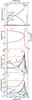 |
Fig. 1 Top panel: principal modes of energy transportation through a J-type shock wave of speed vs = 25 km s-1, propagating into molecular gas of density nH = n(H) + 2n(H2) + n(H+) = 105 cm-3, with an initial transverse magnetic field strength B = 31.6μG. Second panel: thermal and density profiles. Third panel: rates of cooling by the main coolants, per unit volume of gas. Bottom panel: fractional abundances of these coolants, relative to nH. |
5.1. J-type shock
The output of a J-type shock wave model with a magnetic field strength parameter b = 0.1, a preshock density nH = 105 cm-3, and shock speed, vs = 25 km s-1, is representative (cf. Appendix B); the radiative transfer of the methanol lines was not included. The thermal profile of this model is shown in Fig. 1, together with the variation of nH; the independent variable is the distance, z. Also shown are the fractional abundances of major coolants and their rates of cooling per unit volume of the gas. The initial rise in temperature occurs over a small but finite distance, determined by the scale length of the artificial viscosity terms in the conservation equations. This scale length, denoted XLL in the file input/input_mhd.in, must be sufficiently small for the heating and compression of the gas to occur adiabatically, in which case the Rankine-Hugoniot relations are satisfied across the “discontinuity”; XLL = 107 cm in these calculations.
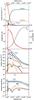 |
Fig. 2 Top panel: principal modes of energy transportation through a C-type shock wave of speed vs = 25 km s-1, propagating into molecular gas of density nH = n(H) + 2n(H2) + n(H+) = 105 cm-3, with an initial transverse magnetic field strength B = 316μG. Second panel: thermal and density profiles. Third panel: rates of cooling by the main coolants, per unit volume of gas. Bottom panel: fractional abundances of these coolants, relative to nH. |
The temperature increases rapidly at the J-“discontinuity”, attaining a maximum value of more than 30 000 K, which is sufficient to dissociate H2. The loss of this major coolant results in a temperature plateau, at about 10 000 K, which lasts until molecular hydrogen reforms, on grain surfaces. The duration of this plateau depends on the value of the probability that H atoms stick to grains, on which H2 forms, at such temperatures; the model adopts the temperature-dependent probability given by Hollenbach & McKee (1979). However, the behaviour of the sticking probability at such high temperatures, at which chemisorption could be important, may be misrepresented by studies aimed at much lower temperatures, at which only physisorption is significant. Thus, the width of the temperature plateau remains uncertain. As may be seen from Fig. 1, the principal coolants are H2, CO, H2O and [O I], with variations arising from the collisional dissociation and the reformation of H2, and the formation and destruction of H2O in the reactions  (1)and
  (2)
(2)
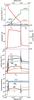 |
Fig. 3 Top panel: principal modes of energy transportation through a CJ-type shock wave of speed vs = 25 km s-1, propagating into molecular gas of density nH = n(H) + 2n(H2) + n(H+) = 105 cm-3 with an initial transverse magnetic field strength B = 316μG. Second panel: thermal and density profiles. Third panel: rates of cooling by the main coolants, per unit volume of gas. Bottom panel: fractional abundances of these coolants, relative to nH. The J-discontinuity is introduced at 250 yr. |
5.2. C-type shock
The output of a C-type shock wave model with a magnetic field strength parameter b = 1.0, a preshock density nH = 105 cm-3, and shock speed, vs = 25 km s-1, is representative (cf. Appendix B); the radiative transfer of the methanol lines was not included in these calculations. The thermal and density profiles of this model are shown in Fig. 2, together with the rates of cooling of the gas by and the fractional abundances of major coolants.
The maximum temperature that is attained is much lower than in an equivalent J-type model, owing to the decoupling of the flow of the charged and neutral fluids induced by the (transverse) magnetic field. As a consequence, the fraction of atomic hydrogen x(H) = n(H)/ [n(H) + 2n(H2) + n(H+)] ≲ 10-3, and hence the rates of the reverse reactions (1) and (2), which convert H2O back to H2 and O, remain negligible. Consequently, the rate of cooling of the gas by the [O I] lines is insignificant.
5.3. CJ-type shock
The output of a CJ-type shock wave model with a magnetic field strength parameter b = 1.0, a preshock density nH = 105 cm-3, and shock speed, vs = 25 km s-1, is representative; the radiative transfer of the methanol lines was not included in these calculations. The dynamical age of this model is 250 yr. The thermal and density profiles of this model are shown in Fig. 3, together with the rates of cooling of the gas by and the fractional abundances of major coolants.
5.4. Energy transportation
As mentioned in Sect. 2.8, the main forms of energy that are transported through the shock structure are kinetic, thermal, magnetic, viscous, internal, and (ultimately) most of the macroscopic kinetic energy of the flow is converted into radiation; the corresponding energy fluxes (erg cm-2 s-1) are plotted in Figs. 1–3 for the three models, J-type, C-type, and CJ-type, respectively. In the case of the C-type shock wave, the viscous contribution is negligible, as there is no “discontinuity” in the flow. Energy conservation requires that the sum of all contributions should remain constant.
1 eV ≡ 11 605 K.
Acknowledgments
It is a pleasure to thank Jacques Le Bourlot, Sylvie Cabrit, David Wilgenbus, Pierre Hily-Blant, Antoine Gusdorf, Caroline McCoey and Delphine Hardin for their contributions to the development of mhd_vode. We thank also the referee for his/her constructive comments. DRF acknowledges support from STFC (ST/L00075X/1), including provision of local computing resources.
References
- Abgrall, H., Roueff, E., & Drira, I. 2000, A&AS, 141, 297 [NASA ADS] [CrossRef] [EDP Sciences] [Google Scholar]
- Ciolek, G. E., Roberge, W. G., & Mouschovias, T. C. 2004, ApJ, 610, 781 [NASA ADS] [CrossRef] [Google Scholar]
- Codella, C., Lefloch, B., Ceccarelli, C., et al. 2010, A&A, 518, L112 [NASA ADS] [CrossRef] [EDP Sciences] [Google Scholar]
- Draine, B. T. 1980, ApJ, 241, 1021 [NASA ADS] [CrossRef] [Google Scholar]
- Flower, D. R. 2010, Flows in Molecular Media, in Jets from Young Stars IV: from Models to Observations and Experiments, eds. P. J. V. Garcia, & J. M. Ferreira (Berlin–Heidelberg: Springer) Lect. Notes Phys., 793 [Google Scholar]
- Flower, D. R., & Pineau des Forêts, G. 2003, MNRAS, 343, 390 [NASA ADS] [CrossRef] [Google Scholar]
- Flower, D. R., & Pineau des Forêts, G. 2012, MNRAS, 421, 2786 [NASA ADS] [CrossRef] [Google Scholar]
- Flower, D. R., & Pineau des Forêts, G. 2013, MNRAS, 436, 2143 [NASA ADS] [CrossRef] [Google Scholar]
- Flower, D. R., Le Bourlot, J., Pineau des Forêts, G., & Cabrit, S. 2003, MNRAS, 341, 70 [NASA ADS] [CrossRef] [Google Scholar]
- Gear, C. W. 1971, Numerical Initial Value Problems in Ordinary Differential Equations (Englewood Cliffs, NJ: Prentice-Hall) [Google Scholar]
- Heck, L., Flower, D. R., Pineau des Forêts, G., & Flower, D. R. 1990, Comp. Phys. Comm., 58, 169 [NASA ADS] [CrossRef] [Google Scholar]
- Herczeg, G. J., Karska, A., Bruderer, S., et al. 2012, A&A, 540, A84 [NASA ADS] [CrossRef] [EDP Sciences] [Google Scholar]
- Hindmarsh, A. C. 1983, in Scientific Computing, eds., R. S. Stepleman, et al. (Amsterdam: North-Holland), 55 [Google Scholar]
- Hollenbach, D., & McKee, C. F. 1979, ApJS, 41, 555 [NASA ADS] [CrossRef] [Google Scholar]
- Le Bourlot, J., Pineau des Forêts, G., & Flower, D. R. 1999, MNRAS, 305, 802 [NASA ADS] [CrossRef] [Google Scholar]
- Lefloch, B., Cabrit, S., Codella, C., et al. 2010, A&A, 518, L113 [NASA ADS] [CrossRef] [EDP Sciences] [Google Scholar]
- Lesaffre, P., Chièze, J.-P., Cabrit, S., & Pineau des Forêts, G. 2004, A&A, 427, 147 [NASA ADS] [CrossRef] [EDP Sciences] [Google Scholar]
- Mathis, J. S., Rumpl, W., & Nordsieck, K. H. 1977, ApJ, 217, 425 [NASA ADS] [CrossRef] [Google Scholar]
- Mullan, D. J. 1971, MNRAS, 153, 145 [NASA ADS] [Google Scholar]
- Neufeld, D., & Kaufman, M. J. 1993, ApJ, 418, 263 [NASA ADS] [CrossRef] [Google Scholar]
- Nisini, B., Benedettini, M., Codella, C., et al. 2010, A&A, 518, L120 [NASA ADS] [CrossRef] [EDP Sciences] [Google Scholar]
- Pineau des Forêts, G., Flower, D. R., Hartquist, T. W., & Dalgarno, A. 1986, MNRAS, 220, 801 [NASA ADS] [CrossRef] [Google Scholar]
- Pineau des Forêts, G., Flower, D. R., Aguillon, F., Sidis, V., & Sizun, M. 2001, MNRAS, 323, L7 [NASA ADS] [CrossRef] [Google Scholar]
- Press, W. H., Teukolsky, S. A., Vetterling, W. T., & Flannery, B. P. 1996, Numerical Recipes in Fortran 90 (Cambridge, UK: Cambridge University Press) [Google Scholar]
- Richtmyer, R. D., & Morton, K. W. 1957, Difference Methods for Initial Value Problems (New York, NY: John Wiley & Sons) [Google Scholar]
- Tappe, A., Forbrich, J., Martinín, S., Yuan, Y., & Jada, C. J. 2012, ApJ, 751, 9 [NASA ADS] [CrossRef] [Google Scholar]
- Wampfler, S. F., Bruderer, S., Karska, A., et al. 2013, A&A, 552, A56 [NASA ADS] [CrossRef] [EDP Sciences] [Google Scholar]
- Wardle, M. 1990, MNRAS, 246, 98 [NASA ADS] [Google Scholar]
- Wrathmall, S., Gusdorf, A., & Flower, D. R. 2007, MNRAS, 382, 133 [NASA ADS] [CrossRef] [Google Scholar]
Appendix A: Grids of shock-wave models for interpreting the spectra of molecular outflow sources
The outflows associated with low-mass star formation have been observed extensively in recent years, by means of ground-based and orbiting observatories. These sources emit in the infrared, millimeter and radio parts of the electromagnetic spectrum (cf. Codella et al. 2010; Lefloch et al. 2010; Nisini et al. 2010; Tappe et al. 2012). Their emission is powered by the outflow, which generates shock waves in the ambient medium and also in the jet. By interpreting these observations, it is possible to derive information on the physical and chemical properties of the medium, the energetics of the outflow, and, ultimately, the process of star formation itself (cf. Flower et al. 2012; 2013; Herczeg et al. 2012; Wampfler et al. 2013).
Shock waves in the interstellar medium may be of “jump” (J) or “continuous” (C) types, depending on the strength of the magnetic field and the degree of ionization in the medium into which the shock wave propagates. If dynamical steady state has not yet been attained – a situation that may often obtain in outflow sources – the shock waves have combined J- and C-type characteristics. In order to relate the dynamics to the emission line spectra, it is essential to treat comprehensively the chemistry of the medium, which comprises gas and dust, and the physical processes of collisional excitation and de-excitation and radiative decay that determine the emission line intensities. Because of the computational demands, previous numerical models of shock waves in the interstellar medium (Mullan 1971; Hollenbach & McKee 1979; Draine 1980; Wardle 1990; Neufeld & Kaufman 1993; Ciolek et al. 2004; Lesaffre et al. 2004) have emphasized either the dynamics, at the expense of the chemical and physical micro-processes, or vice versa. Our own model inclines towards a comprehensive treatment of the micro-processes, whilst retaining the principal aspects of the dynamics.
In order to assist with the interpretation of observations of outflows, we have generated and are now making available a grid of shock-wave models, whose predicted spectra may be compared with the observed atomic and molecular line intensities. We shall discuss the results of these computations in terms of the total energy emitted by the principal cooling species. This approach enables the main coolants to be identified, as the parameters of the shock wave vary, whilst avoiding the minutiae of the spectral line emission. However, complete spectral information is available for all the models comprising the grid.
It will be appreciated that calculations of this type involve a large number of explicit and implicit parameters, The explicit parameters are the initial values of the dynamical variables: the flow speeds, temperatures, number densities and mass densities of each of the fluids; the initial magnetic field strength, perpendicular to the direction of the flow; and the initial values of the abundances of the chemical species and of the level population densities, as mentioned above (Sect. 2.19). The implicit parameters are the rate coefficients incorporated in the chemical reaction network (which contains, typically, of the order of a thousand reactions) and the spectroscopic, radiative and collisional data pertaining to the atomic and molecular coolants. The discussion of the results in Appendix B will focus on the initial values of certain key parameters; but the complexities of the problem and its solution need to be borne in mind.
Appendix B: Results and discussion
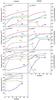 |
Fig. B.1 Total rate of cooling by the main molecular coolants, as a function of the shock speed and for the preshock densities, nH = n(H) + 2n(H2) + n(H+), indicated. Results for both C- and J-type shock models are shown. |
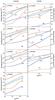 |
Fig. B.2 As Fig. B.1, but as a function of nH = n(H) + 2n(H2) + n(H+) and for the shock speeds, vs, indicated. Results for both C- and J-type shock models are shown. |
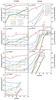 |
Fig. B.3 Total rate of cooling by the main atomic and ionic coolants, as a function of the shock speed and for the preshock densities, nH = n(H) + 2n(H2) + n(H+), indicated. Results for both C- and J-type shock models are shown. |
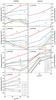 |
Fig. B.4 As Fig. B.3, but as a function of nH = n(H) + 2n(H2) + n(H+) and for the shock speeds, vs, indicated. Results for both C- and J-type shock models are shown. |
The grids of C- and J-type models cover a range of shock speeds (10 ≤ vs ≤ 40 km s-1) and preshock densities, nH = n(H) + 2n(H2) + n(H+) (103 ≤ nH ≤ 106 cm-3). The transverse magnetic field strength scales with the density through the relation ![Mathematical equation: \appendix \setcounter{section}{2} \begin{eqnarray*} B(\mu {\rm G}) = b[n_{\rm H} ({\rm cm}^{-3})]^{\frac {1}{2}}. \end{eqnarray*}](/articles/aa/full_html/2015/06/aa25740-15/aa25740-15-eq106.png) We adopted b = 1.0 for C-type and b = 0.1 for J-type models, which is consonant with larger field strengths being necessary to generate C-type shock waves. The range of J-type models does not extend beyond vs = 35 km s-1 and nH = 105 cm-3, at which the dissociation of H2 becomes complete and the collapse of the radiative cooling of the medium results in a thermal runaway. In Fig. B.1 is shown the integrated flux of radiation that is emitted by significant cooling molecules (H2, CO, H2O, NH3, OH), as a function of the shock speed, for both the C-type and the J-type models. Analogous plots, as functions of nH, are presented in Fig. B.2. Tables of the integral atomic and molecular line intensities – or, in the case of H2, values of column densities, divided by the level degeneracies – extracted at the point at which the temperature of the postshock gas has fallen to 15 K, are provided in ASCII format at the CDS.
We adopted b = 1.0 for C-type and b = 0.1 for J-type models, which is consonant with larger field strengths being necessary to generate C-type shock waves. The range of J-type models does not extend beyond vs = 35 km s-1 and nH = 105 cm-3, at which the dissociation of H2 becomes complete and the collapse of the radiative cooling of the medium results in a thermal runaway. In Fig. B.1 is shown the integrated flux of radiation that is emitted by significant cooling molecules (H2, CO, H2O, NH3, OH), as a function of the shock speed, for both the C-type and the J-type models. Analogous plots, as functions of nH, are presented in Fig. B.2. Tables of the integral atomic and molecular line intensities – or, in the case of H2, values of column densities, divided by the level degeneracies – extracted at the point at which the temperature of the postshock gas has fallen to 15 K, are provided in ASCII format at the CDS.
Figures B.1 and B.2 show that, in the C-type models, the main molecular coolants of the shocked gas are H2, H2O, CO, and NH3; radiative cooling by OH is relatively unimportant. The fluxes of radiation emitted by the main coolants are approximately proportional to the preshock density, as may be deduced from Fig. B.2; this reflects the proportionality of the kinetic energy flux of the shock wave,  , to the initial density, and the fact that much of this kinetic energy is ultimately converted into radiation that is emitted by the gas. The maximum temperatures that are attained in C-type shocks are sufficient to drive the formation of H2O, in the successive reactions H2(O, OH)H and H2(OH, H2O)H, but are insufficient to give rise to appreciable collisional dissociation of molecular hydrogen. Consequently, the reverse reactions, with H, are unable to elevate the fractional abundances of OH and O in the gas. In the corresponding J-type shocks, on the other hand, much higher maximum temperatures are produced, thereby dissociating H2 to H and modifying the chemical balance in favour of the reverse reactions and ensuring that OH (and O: see below) become significant coolants.
The rates of cooling by atoms and ions are presented in Figs. B.3 and B.4, where it may be seen that [S I] and [O I] transitions are the main contributors. The predominance of S is attributable to its high fractional abundance in the preshock gas and to its chemical stability, even under the conditions in shock waves. The  →
→ 25.2 μm transition of [S I] was observable by means of the Spitzer infrared spectrograph (cf. Tappe et al. 2012), but neither this nor the
  →
→ transition at 56.3 μm can currently be observed.
The atomic hydrogen that is produced in the J-type shocks is partially ionized to H+, in collisions with hot electrons. The free electrons that are produced can excite the bound electrons of H2 and H; collisional excitation is followed by radiative decay and loss of energy from the medium, The net effect is to cool the electrons, which are thermally coupled to the ions and neutrals by elastic scattering. This process becomes the most important cooling mechanism at high shock speeds, for which the maximum temperatures are greatest.
In practice, observations of only a limited selection of atomic and molecular species are available for any given outflow source. The smaller the number of species, the more it becomes necessary to rely on comparisons of transitions emitted from several energy levels of a given species, with differing degrees of excitation, when deducing shock-wave parameters. With this consideration in mind, we include complete sets of information on the intensities of all transitions emitted by the species that are included in the C-type2 and J-type3 models of the grid.
All Figures
|
Fig. 1 Top panel: principal modes of energy transportation through a J-type shock wave of speed vs = 25 km s-1, propagating into molecular gas of density nH = n(H) + 2n(H2) + n(H+) = 105 cm-3, with an initial transverse magnetic field strength B = 31.6μG. Second panel: thermal and density profiles. Third panel: rates of cooling by the main coolants, per unit volume of gas. Bottom panel: fractional abundances of these coolants, relative to nH. |
| In the text | |
|
Fig. 2 Top panel: principal modes of energy transportation through a C-type shock wave of speed vs = 25 km s-1, propagating into molecular gas of density nH = n(H) + 2n(H2) + n(H+) = 105 cm-3, with an initial transverse magnetic field strength B = 316μG. Second panel: thermal and density profiles. Third panel: rates of cooling by the main coolants, per unit volume of gas. Bottom panel: fractional abundances of these coolants, relative to nH. |
| In the text | |
|
Fig. 3 Top panel: principal modes of energy transportation through a CJ-type shock wave of speed vs = 25 km s-1, propagating into molecular gas of density nH = n(H) + 2n(H2) + n(H+) = 105 cm-3 with an initial transverse magnetic field strength B = 316μG. Second panel: thermal and density profiles. Third panel: rates of cooling by the main coolants, per unit volume of gas. Bottom panel: fractional abundances of these coolants, relative to nH. The J-discontinuity is introduced at 250 yr. |
| In the text | |
|
Fig. B.1 Total rate of cooling by the main molecular coolants, as a function of the shock speed and for the preshock densities, nH = n(H) + 2n(H2) + n(H+), indicated. Results for both C- and J-type shock models are shown. |
| In the text | |
|
Fig. B.2 As Fig. B.1, but as a function of nH = n(H) + 2n(H2) + n(H+) and for the shock speeds, vs, indicated. Results for both C- and J-type shock models are shown. |
| In the text | |
|
Fig. B.3 Total rate of cooling by the main atomic and ionic coolants, as a function of the shock speed and for the preshock densities, nH = n(H) + 2n(H2) + n(H+), indicated. Results for both C- and J-type shock models are shown. |
| In the text | |
|
Fig. B.4 As Fig. B.3, but as a function of nH = n(H) + 2n(H2) + n(H+) and for the shock speeds, vs, indicated. Results for both C- and J-type shock models are shown. |
| In the text | |
Current usage metrics show cumulative count of Article Views (full-text article views including HTML views, PDF and ePub downloads, according to the available data) and Abstracts Views on Vision4Press platform.
Data correspond to usage on the plateform after 2015. The current usage metrics is available 48-96 hours after online publication and is updated daily on week days.
Initial download of the metrics may take a while.