| Issue |
A&A
Volume 578, June 2015
|
|
|---|---|---|
| Article Number | A45 | |
| Number of page(s) | 19 | |
| Section | Catalogs and data | |
| DOI | https://doi.org/10.1051/0004-6361/201424676 | |
| Published online | 02 June 2015 | |
E-BOSS: An Extensive stellar BOw Shock Survey
II. Catalogue second release
1 Instituto Argentino de Radioastronomía, CCT-La Plata (CONICET), C.C.5, 1894 Villa Elisa, Argentina
e-mail: cperi@fcaglp.unlp.edu.ar
2 Facultad de Ciencias Astronómicas y Geofísicas, UNLP, Paseo del Bosque s/n, 1900 La Plata, Argentina
Received: 24 July 2014
Accepted: 17 February 2015
Context. Stellar bow shocks have been studied not only observationally, but also theoretically since the late 1980s. Only a few catalogues of them exist. The bow shocks show emission along all the electromagnetic spectrum, but they are detected more easily in infrared wavelengths. The release of new and high-quality infrared data eases the discovery and subsequent study of new objects.
Aims. We search stellar bow-shock candidates associated with nearby runaway stars, and gather them together with those found elsewhere, to enlarge the list of the E-BOSS first release. We aim to characterize the bow-shock candidates and provide a database suitable for statistical studies. We investigate the low-frequency radio emission at the position of the bow-shock features, that can contribute to further studies of high-energy emission from these objects.
Methods. We considered samples from different literature sources and searched for bow-shaped structures associated with stars in the Wide-field Infrared Survey Explorer (WISE) images. We looked for each bow-shock candidate on centimeter radio surveys.
Results. We reunited 45 bow-shock candidates and generated composed WISE images to show the emission in different infrared bands. Among them there are new sources, previously studied objects, and bow shocks found serendipitously. Five bow shocks show evidence of radio emission.
Conclusions. Stellar bow shocks constitute an active field with open questions and enormous amounts of data to be analyzed. Future research at all wavelengths databases, and use of instruments like Gaia, will provide a more complete picture of these objects. For instance, infrared spectral energy distributions can give information about physical parameters of the bow shock matter. In addition, dedicated high-sensitivity radio observations can help to understand the radio-γ connection.
Key words: catalogs / stars: early-type / infrared: ISM
© ESO, 2015
1. Introduction
High-mass stars interact with the interstellar medium (ISM) producing different kinds of observable structures. An important proportion of early-type (OB) stars are runaway and have high velocities with respect to the normal stars, nearby ISM, and mean Galactic rotation speed (Blaauw 1961; Gies & Bolton 1986; Gies 1987; Stone 1991; Tetzlaff et al. 2011; Fujii & Portegies Zwart 2011).
Some runaway stars generate the so-called stellar bow shocks, a comma-shaped source usually detected in front of the star trajectory. The stellar motion with respect to the ISM helps to accumulate the matter ahead of the star, and the stellar ultraviolet radiation field heats the dust that emits infrared (IR) photons (e.g., van Buren & McCray 1988; Noriega-Crespo et al. 1997; Kobulnicky et al. 2010; Gvaramadze et al. 2014). Additionally, the supersonic motion of a star produces shock waves, and through mechanisms like Fermi of first order, the charged particles can be accelerated up to relativistic velocities. These particles can interact with different fields − matter, magnetic, or photon fields − and produce high energy and radio emission (Benaglia et al. 2010; del Valle & Romero 2012, 2014; del Valle et al. 2013; López-Santiago et al. 2012). The stellar UV field also ionizes the gas, which recombines and emits photons in the optical range (Brown & Bomans 2005; Gull & Sofia 1979).
The infrared luminosity of stellar bow shocks is high compared to those in other spectral bands (e.g., Benaglia et al. 2010, Fig. 5; del Valle & Romero 2012, Fig. 11; Benaglia 2012, Table 1). Stellar bow shocks are in principle not difficult to discover at IR frequencies if they are close to us − no farther than a few kpc − and not very dim.
Group 3: Tetzlaff WISE 2.
Among the first results of the InfraRed Astronomical Satellite (IRAS, Neugebauer et al. 1984), the first list of stellar bow shocks was published in the late 1980s. Noriega-Crespo et al. (1997) found 19 bow-shock candidates (BSCs, hereafter) and 2 doubtful objects among 58 high-mass runaway stars. The Wide-field Infrared Survey Explorer (WISE, Wright et al. 2010) satellite data release offered a sensitive arcsec resolution mid-infrared all-sky survey. In 2012, Peri et al. (2012) published the first release of the catalogue called E-BOSS: an Extensive stellar BOw Shock Survey (hereafter E-BOSS r1), done by searching these sources mainly in the then available WISE images (57% of the sky). The final product was made up of a list of 28 BSCs, and minor studies of them in radio and optical wavelengths.
In this paper, we present the E-BOSS second release (hereafter E-BOSS r2), where we extended the search to more samples. The sources taken into account are described in Sect. 2; the different databases used to perform the search in Sect. 3; and the results, including the final BSCs release 2 list, in Sect. 4. Section 5 presents a discussion and Sect. 6 closes with a summary and conclusions.
2. Data samples: organization of the groups
E-BOSS first release (r1, Peri et al. 2012) was based on two samples. Group 1 consisted of a set of sources taken from Noriega-Crespo et al. (1997) and Group 2 was a list extracted from Tetzlaff et al. (2011). To build the present and second E-BOSS release (r2) we used samples extended to other spectral types, sources with no public WISE data at the moment of making E-BOSS r1, bow shocks from the literature, and bow shocks found serendipitously. In order to avoid confusion about the group numbers of r1 and r2, we begin here with Group 3. We give a first approximation for each group origin in this section; then we give a detailed analysis in the Results section.
2.1. Group 3
Tetzlaff et al. (2011) generated a catalogue of runaway stars using as the main source the Hipparcos stellar catalogue (van Leeuwen 2007). The authors selected 7663 young stars up to 3 kpc from the Sun; completed the radial velocities from literature; studied peculiar spatial, radial, and tangential velocities; and estimated the runaway probability for each star of the sample. In addition, they investigated some stars that showed high velocities with respect to their environment. Previous works analyzed the runaway origin of the high-velocity stars taking into account only peculiar spatial velocities (Blaauw 1961; Gies & Bolton 1986), radial velocities (Cruz-González et al. 1974), or tangential velocities (Moffat et al. 1998). Instead, Tetzlaff et al. (2011) combined all the available criteria and give a list of 2547 runaway stars, increasing the amount of sources in two orders of magnitude.
Originally, E-BOSS r1 Group 2 included 244 candidates for runaway stars from Tetzlaff et al. (2011). The stellar spectral types range from O to B2, and 80 of them had no public WISE data at the moment of the first release. These 80 stars form Group 3 in this paper. We named the group Tetzlaff WISE 2, because the public IR data corresponds to the second WISE release. The list of Group 3 stars is shown in Table 1.
2.2. Group 4
Group 4 collects stars from Tetzlaff et al. (2011), but with later spectral types with respect to Groups 2 and 3. We selected stars with spectral types from B3 to B5, and called this group Tetzlaff B3-B5. The list is in Table 2 and has a total of 234 stars.
Group 4: Tetzlaff B3-B5.
Group 5: GOSC.
2.3. Group 5
Maíz-Apellániz et al. (2004) produced an O galactic star catalogue, and classified 42 of them as runaways. We created Group 5, GOSC, with these 42 objects, and show the list in Table 3. There are two subgroups in Group 5; the first corresponds to stars already analyzed in E-BOSS r1, and the second to stars studied in this paper.
2.4. Group 6
Hoogerwerf et al. (2001) have studied the dynamic origin of 56 runaway stars and 9 pulsars. Of the 56 stars, we eliminated those coincident with the rest of the groups (from 1 to 5), and find 10 new objects to analyze. The list is presented in Table 4, labeled as Group 6, and named Hoogerwerf et al. (2001).
Group 6: Hoogerwerf et al. (2001).
Group 7: Serendipity and literature.
2.5. Group 7
We built Group 7 with BSCs already analyzed by colleagues (38 objects) and BSCs that appeared serendipitously in the IR images during our searches (7 objects). This group is called “Serendipity and literature”. In Table 5, we enumerate the objects, list the identification in the original work (whenever possible), and characterize the WISE emission. The first column shows the name we gave to the sources in this group. We used the prefix G7 for each object and added a number that goes from 01 to 45. The last column has a comment about the region, or important information from the cited papers or added by us.
For Groups from 2 to 6 we selected runaway stars and searched for BSCs around them. In Group 7 (and Group 1, from r1) this criterion was not valid; the BSCs structures were discovered directly by us or by other authors.
2.6. Wolf-Rayet stars
The Tetzlaff et al. (2011) catalogue includes a group of Wolf-Rayet stars in the analysis of possible runaway stars. The authors list as runaways the 18 stars WR 2, 11, 15, 24, 31, 46, 47, 52, 66, 79, 110, 111, 121, 136, 138, 139, 153, and 156 (see van der Hucht 2001 for coordinates). We looked for IR bow-shaped emission at the WISE image cutouts and found no BSC related to the mentioned stars. The findings can be summarized as emission from discrete sources (WR 24, WR 153), high noise level (WR 111), wind bubble (WR 136 related to NGC 6888), and no emission above the noise for the rest of the runaway WR stars.
3. Searches
Previous evidence showed that stellar bow shocks have high infrared luminosity (e.g., Benaglia et al. 2010, Fig. 5; del Valle & Romero 2012, Fig. 11; Benaglia 2012, Table 1) compared to those in other wavelengths, which is why we aimed the search at infrared frequencies. The WISE second release (Wright et al. 2010) was published after E-BOSS r1 and completed the all-sky survey, allowing us to continue with BSCs studies.
We made use of the InfraRed Science Archive service1 (IRSA/IPAC NASA), and performed the search seeking a bow-shock shape in front of each selected runaway star or BSC already observed, for all the r2 Groups (3 to 7). We looked for the BS structure for each source in WISE four bands, and used the FITS images already processed. The extent of the fields was one square degree. At least two authors inspected the results.
We show a RGB (red-green-blue) composed image of the resulting BSCs, except those cases where the sources had an associated WISE image already published. The RGB image shows the emission of the WISE bands 1, 3, and 4 (3.4 μm, 12.1 μm, and 22 μm, respectively). In particular, WISE band 4 is useful for detecting warm dust (Wright et al. 2010).
We investigated the final list of BSCs in radio wavelengths. The case of BD +43° 3654 (Benaglia et al. 2010) is the first BSC with synchrotron emission; we checked whether any of the new BSCs constituted a similar case. We looked for BSCs in the NRAO/VLA Sky Survey2 (NVSS, Condon et al. 1998), which returns images of the 1.4 GHz frequency emission in several formats.
4. Results
4.1. Bow-shock candidates: Groups 3 to 6
Group 3, Tetzlaff WISE 2 (Table 1), has 80 objects. We found six BSC and two doubtful cases. Since the group consists of runaway stars, we associated each BSC with a star name. The six cases are: HIP 44368, HIP 47868, HIP 98418, HIP 101186, HIP 104579, and HIP 105186, and are shaded in gray in Table 1. The HIP 101186 region was already studied in E-BOSS r1, but with Midcourse Space Experiment (MSX, Egan et al. 2003) cutouts; no WISE data was available in the zone at that moment. For the six BSC we built RGB images from WISE bands cutouts (Figs. 5 and 6). Cases like HIP 48469 and HIP 111071 have no clear bow-shock shapes in their surroundings; they are separated as special cases (Sect. 4.5) and marked with ∗∗ in Table 1.
Group 4 is also made up of runaway stars; hence, we use the star names to identify the BSCs. We found 3 BSCs and 13 special cases; they are shaded in gray and marked with ∗∗, respectively, in Table 2. The BSCs are related to HIP 17358, HIP 46928, and HIP 107789. HIP 17358 was already analyzed in E-BOSS r1. Figure 6 shows HIP 46928 and 107789. Additionally, we encountered two bow-shock features not associated with the stars in Group 4, but in the stellar fields of HIP 5569 and HIP 33987. They will be presented in next section (Figs. 10 and 11).
In Group 5 we found evidence of one BSC, identified around HD 57682. The source is shaded in gray in Table 3 and presented in Fig. 6. We found one BSC in Group 6 associated with HIP 86768 (Fig. 6) and one special case around HIP 102274. Both cases are marked in Table 4, in gray and with ∗∗ respectively.
List of the E-BOSS release 2 bow-shock candidates and corresponding stellar parameters.
4.2. Bow-shock candidates: Group 7
Group 7 BSCs are shown in Table 5. Povich et al. (2008) reported the discovery of six infrared stellar wind bow shocks in the galactic massive star-forming regions M17 and RCW 49 from Spitzer GLIMPSE (Galactic Legacy Infrared Mid-Plane Survey Extraordinaire, Benjamin et al. 2003) images. We searched for them in the WISE image database. The images looked saturated, except for the BSC RCW 49 S1 (Fig. 7).
Kobulnicky et al. (2010) found ten stellar bow shocks among Spitzer images, in the Cygnus OB2 association, at the heart of the Cygnus-X region. An extra case is the star BD +43° 3654, studied by Comerón & Pasquali (2007), for which the authors confirm its runaway nature, but display no image. We found each BSC in WISE images, but BSCs numbers 8 and 9 are doubtful cases (Sect. 4.5). We show WISE images in Figs. 7 and 8, and add the BSCs in the final E-BOSS r2 list. The WISE first release did not cover the region of BD +43° 3654, and we show the RGB WISE composite image in this work (Fig. 8).
The next eight BSCs are located near two young clusters associated with the star-forming region NGC 6357 (Gvaramadze et al. 2011a). Seven were discovered in MSX, Spitzer, and WISE images. The authors presented one BSC with WISE images; hence, we constructed images for the other seven (Figs. 8 and 9) and included all eight in the E-BOSS r2 final list.
The structure and kinematics of the ISM around the runaway star HD 192281 was studied by Arnal et al. (2011). The authors found signs of the star trajectory using Canadian Galactic Plane Survey (CGPS, Taylor et al. 2003) and MSX images. We looked for similar structures in WISE images but no clear feature was found. In addition, we looked for a comma-shaped or similar emission, but with no success.
Vela X-1 (HIP 44368, Group 3) is the first case of a runaway high-mass X-ray binary (HMXB) showing a bow-shock structure ahead of its motion direction (Kaper et al. 1997). We include this source on E-BOSS r2. The star 4U 1907+09 is also a runaway object (Gvaramadze et al. 2011c) and presents a bow-shock feature (Fig. 10). This is the second BSC associated with an HMXB. 4U 1700-37 is a runaway HMXB too (Ankay et al. 2001). We did not find a clear comma-shaped structure ahead of the star in any of the WISE bands.
Gvaramadze et al. (2013) studied two massive stars possibly ejected from the NGC 3603 cluster through dynamical few-body encounters. The authors showed Spitzer images of the surroundings of the star J1117-6120 and its suspected original companion (a O2 If*/WN6 star, WR42e). We constructed a RGB WISE image for J1117-6120 (Fig. 10); for WR42e, the field is saturated.
Optical spectroscopy for the runaway blue supergiant TYC 3159-6-1 star was presented by Gvaramadze et al. (2014), together with a discussion that assumes Dolidze 7 to be its parent cluster (Cygnus-X region). The authors show a band 3 (12 μm) WISE image. We include the TYC 3159-6-1 nebulae as a BSC (Table 5).
Three BSCs were analyzed by Gvaramadze & Bomans (2008) near the NGC 6611 cluster, located in the Ser OB 1 association. NGC 6611 has possibly ejected three of its O massive stars: BD −14° 5040, HD 165319, and “star 1”. HD 165319 (HIP 88652) was part of E-BOSS r1. For BD −14° 5040 and “star 1”, we generated RGB WISE images (Fig. 10) and included them in the E-BOSS r2 list (Table 6).
Sources G7 35 to 38 (Table 5) were shown in a Hubblesite News Center release3. We named the objects H1, H2, H3, and H4. Observations made by R. Sahai (HST Cycle 14 proposal 10536), using the ACS SNAPshot Survey of the HST between 2005 and 2006, were dedicated to a survey of preplanetary nebulae candidates (Sahai et al. 2007). Among the observed sources, Sahai and his team found what seemed to be four BSC.
Parameters of the bow-shock candidates and medium density.
Liu et al. (2011) developed a thorough study of the young cluster associated with the Circinius molecular cloud, and uncovered a population of YSOs in the western region of the cloud. The authors found two aggregates of YSOs, and H1 is located in the middle region between both YSO groups. Several sources from different works and wavelengths are mixed inside the WISE source associated with H1, like the Herbig-Haro object 139. Although HH 139 is embedded in the WISE source, H1 is about 4 arcsec from HH 139 at optical wavelengths. We do not have sufficient evidence yet to confirm the stellar bow-shock nature of H1.
Source H2 seems to be related to the infrared source IRAS 20193+3448, its nearest source. This source was identified as “a likely transitional YSO” (Magnier et al. 1999). If H2 is related to IRAS 20193+3448 and its surroundings, we rule out that it is a BSC, because the whole region is related to a star-forming region.
Sahai et al. (2012) published a multi-wavelength study of the source IRAS 20324+4057 and some surrounding structures; all of them near H3. They conclude the sources were dense molecular cores originated in the Cygnus cloud. Therefore, we excluded H3 as a possible BSC like the ones we are looking for.
In Hubble images H4 has a boomerang shape, but the WISE source covers several times the optical one. There is no catalogued source around H4 on about 30 arcsec; therefore, we cannot discard the boomerang as a BSC.
Hubble Space Telescope has an angular resolution of 0.05 arcsec, and WISE between 6.1 and 12 arcsec depending on the band. For all the cases (H1, H2, H3, and H4), the IR sources are unresolved. Several optical sources can contribute to the IR emission. Only H4 remains as a possible BSC.
The last seven cases in Table 5 (G7 39 to 45) are serendipity BSCs. We found them in WISE images during the searches. We called the objects SER 1 to 7. SER 1 (Fig. 10) seems to have been generated by the TYC 7688-424-1 star according to Simbad sources (spectral type B5Ve). For SER 2 (Fig. 10) we do not find any catalogued star to be considered as a bow-shock producer. SER 3 (Fig. 11) could be related to HD 303197, according to Simbad. HD 303197 (spectral type B5) is located near the NGC 3324 open cluster, although the bow-shock shape seems to indicate that the star might be coming from another direction, towards the cluster. SER 4 (Fig. 11) could be produced by HIP 117265 (spectral type B2IV). SER 5 (Fig. 11) can be generated by HIP 34301 (TYC 5389-3064-1), or BD-11 1790C (double system). For SER 6 (Fig. 11) we did not find a star that might produce the BSC. SER 7 (Fig. 11) has no clear star related to it; the nearest stars are HD 153426 (80.6′′), and HD 322486 (102.2′′), and they are not located where runaway stars usually lie to cause a bow-shock structure.
4.3. Bow-shock candidates list
In Table 6 we list the final set of new BSCs that we found, together with those already analyzed by other authors. In E-BOSS release 2 there are 45 new objects in addition to those of release 1. The first column of Table 6 gives the name of the star that generates the BSC whenever identification was possible, or another name when the star cannot be determined. The second column contains the Group number and the third column the galactic coordinates (of stars or stagnation point), from Simbad or reference from Table 5. The stellar spectral types were taken from Simbad (B-type), the GOS Catalog (Maíz-Apellániz et al. 2004), or the reference from Table 5. The distances were taken from Megier et al. (2009), Mason et al. (1998) or were estimated using parallaxes from Hipparcos (van Leeuwen 2007). The stellar wind terminal velocities were interpolated or extrapolated from Table 3, Prinja et al. (1990), or adopted as in Peri et al. (2012) for stars with the same spectral types. The mass-loss rates were interpolated or extrapolated from Vink et al. (2001). The tangential velocity of HIP 44368 was estimated through proper motion values, and for the other sources of Groups 3 and 4 the values are from Tetzlaff et al. (2011). Radial velocities for Groups 3 to 6 are from Kharchenko et al. (2007); for objects in Group 7, references are as in Table 5, and Simbad for SER 1, 3, 4, and 5. Proper motions of stars in Groups 3 to 6 and K3 (HD 195229) are from Hipparcos (van Leeuwen 2007), and for G1 to G8 we show two values from Gvaramadze et al. (2011a); for TYC 3159-6-1, BD −14 5040, and Star 1, references are as in Table 5 (see errors for velocities and proper motions in references); for SER 1, 3, 4, and 5, Simbad.
4.4. Bow-shock candidate features
Table 7 shows the measured sizes of the bow-shock candidates. We list the length l and width w of each bow-shock structure, and distance R from the star to what is known as stagnation point (Wilkin 1996), in angular units. The sizes were taken from WISE band 4 or band 3 images. Whenever possible, we also estimated l, w, and R on linear units (pc) through distance measurements. No size is given for cases without WISE images.
The ISM ambient density was derived for the bow-shock candidates with adopted distances and stellar spectral types, as in Peri et al. (2012). To this aim, we used the expression that gives the stagnation radius R0: 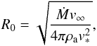 where ρa = μnISM is the ambient medium density, and v∗ is the spatial stellar velocity. The volume density of the ISM is in H atoms at the bow-shock position assuming R0 ~ R, a mass per H atom μ = 2.3 × 10⁻²⁴ g, and the helium fractional abundance Y = 0.1. For those stars with unknown spatial peculiar velocity we adopted v∗ = 25 km s-1. We show the results in Table 7. Values obtained for nISM must be taken into account with caution: errors on each parameter used in the R0 expression can have a strong influence in calculations.
4.5. Special cases
We found several doubtful cases during the BSCs search. All the special cases are marked with ∗∗ in the tables. The cases are: in Group 3 (Table 1), HIP 48469 and 111071; in Group 4 (Table 2), HIP 3478, 11894, 15114, 30169, 32786, 34485, 43955, 48589, 62913, 76416, 94385, 99618, and 105268; in Group 6 (Table 4), HIP 102274.
In WISE band 4 (22.2 μm) many stars show circular emission around the stellar object which is usually seen in band 1, 3.4 μm. This could indicate that the radial velocity dominates over the tangential one. Other cases show different shapes depending on the WISE band, which makes us wonder if they were BSC emission or something else. In some cases, therefore, the bow shock may still be forming and has not yet achieved the comma-shape.
Group 7 (Table 5) has nine special cases. Two sources are from Kobulnicky et al. (2010): K8 and K9. The stellar bow-shock number 8 is mixed with ISM on WISE images and we did not see a clear comma-shaped object; K9 has, as many of the special cases in this work, circular emission around the star. HD 192281 (Arnal et al. 2011) images of WISE do not show a clear bow-shape either. The last special case is H4. The WISE resolution overcomes the Hubble one, precluding a BSC identification. The BSCs related to G3, G4, G6 (Gvaramadze et al. 2011a), SER3, and SER4 are doubtful cases on the basis of morphology, but we include them on the E-BOSS r2 list because they are candidates.
We do not discard any of the special cases as a probable BSC, but for the reasons stated above, we could not identify them. Subsequent studies can reveal the sources in the future and help to decide their nature.
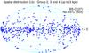 |
Fig. 1 Distribution on the (l,b) plane of Groups 2, 3, 4, 5 and 6. Runaway stars were taken from Tetzlaff et al. (2011) and Hoogerwerf et al. (2001). |
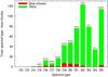 |
Fig. 2 Spectral type histogram for Groups 2 to 6, summarized. Each range of spectral types has the total number of stars in green, the amount of BSCs in red, and the proportion of BSCs according to the total number of sources in each range. We did not include stars of spectral types with no specific subtype (two stars of spectral type Op, and 12 stars of spectral type B). |
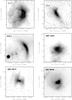 |
Fig. 3 BSCs that show radio emission. Gray scale colors: IR WISE emission (band 4, 22.2 μm). Contours: NVSS 1.4 GHz emission. Positive values in gray, negative in black. Contour levels on each image: top left, −1, 1, 1.5, 2, 5 mJy/b. Top right, −5, 1, 5 mJy/b. Middle left, −1, 1, 1.5, 20, 150 mJy/b. Middle right, −4, 4, 16, 30, 40 mJy/b. Bottom left, −1, 1, 2, 3 mJy/b. Bottom right, −10, 10, 30, 60, 90, 120, 160 mJy/b. |
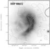 |
Fig. 4 Bow-shock candidate related to HIP 88652 (E-BOSS r1). Gray scale colors: IR WISE emission (band 4, 22.2 μm). Contours: NVSS 1.4 GHz emission. Contour levels: −1, 1, 2, 3 mJy/b. Positive values in gray, negative in black. |
Total list of BSC of E-BOSS r1 and r2.
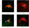 |
Fig. 5 Group 3 bow-shock candidates WISE images. Red: band 4, 22.2 μm. Green: band 3, 12.1 μm. Blue: band 1, 3.4 μm. The label stands for the name in the final list of E-BOSS r2 BSCs. We have drawn μαcosδ and μδ to compose the total μ. The thick vectors represent the measured Hipparcos proper motions (van Leeuwen 2007), and the thinner vectors stand for the star proper motions but corrected for the ISM motion caused by Galactic rotation. The vector lengths are not scaled with the original values. Compass as in HIP 44368 is the same for all RGB images. |
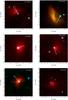 |
Fig. 6 Groups 3, 4, 5, and 6 bow-shock candidates WISE images. Red: band 4, 22.2 μm. Green: band 3, 12.1 μm. Blue: band 1, 3.4 μm. The label stands for the name in the final list of E-BOSS r2 BSCs. We have drawn μαcosδ and μδ to compose the total μ. The thick vectors represent the measured Hipparcos proper motions (van Leeuwen 2007), and the thinner vectors stand for the star proper motions but corrected for the ISM motion caused by Galactic rotation. The vector lengths are not scaled with the original values. |
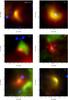 |
Fig. 7 Group 7 bow-shock candidates WISE images. Red: band 4, 22.2 μm. Green: band 3, 12.1 μm. Blue: band 1, 3.4 μm. The label stands for the name in the final list of E-BOSS r2 BSCs. |
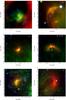 |
Fig. 8 Group 7 bow-shock candidates WISE images. Red: band 4, 22.2 μm. Green: band 3, 12.1 μm. Blue: band 1, 3.4 μm. The label stands for the name in the final list of E-BOSS r2 BSCs. For BD +43° 3654, we have drawn μαcosδ and μδ to compose the total μ. The thick vector represent the measured Hipparcos proper motions (van Leeuwen 2007), and the thinner vectors stand for the star proper motions but corrected for the ISM motion caused by Galactic rotation. The vector lengths are not scaled with the original values. |
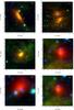 |
Fig. 9 Group 7 bow-shock candidates WISE images. Red: band 4, 22.2 μm. Green: band 3, 12.1 μm. Blue: band 1, 3.4 μm. The label stands for the name in the final list of E-BOSS r2 BSCs. The BSC labeled G 4 has two structures; we have taken the BSC of the northern one because of the location of the star that might have generated it. |
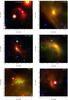 |
Fig. 10 Group 7 bow-shock candidates WISE images. Red: band 4, 22.2 μm. Green: band 3, 12.1 μm. Blue: band 1, 3.4 μm. The label stands for the name in the final list of E-BOSS r2 BSCs. |
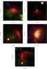 |
Fig. 11 Group 7 bow-shock candidates WISE images. Red: band 4, 22.2 μm. Green: band 3, 12.1 μm. Blue: band 1, 3.4 μm. The label stands for the name in the final list of E-BOSS r2 BSCs. |
4.6. Statistics
We carried out statistical studies for Groups 2 to 6 (E-BOSS r1 and r2) because they share the same search criterion: we looked for BSCs around runaway stars. We studied the spatial distribution and spectral types, and displayed the corresponding plots in Figs. 1 and 2. We built these plots to look for trends related to stellar spectral types or spatial distribution and the presence of BSCs in the star sample.
Figure 1 shows the spatial distribution in galactic coordinates for all the sources of Groups 2 to 6, using two different symbols for the objects with or without BSCs found by us. From this figure we found no clear spatial tendencies for the sources associated with BSCs.
Figure 2 gives the total number of stars for each subspectral type, from O2 to B5, and the proportion of sources with BSCs. We had to exclude several cases; for Group 4 (stars B3-B5) we discarded sources of B type with no subspectral type, and for Group 3 (Tetzlaff WISE 2) we excluded two stars of Op type. It can be seen from the plot that the probability of finding a BSC in the surroundings of B-type stars (~1.2%) is less than that for O-type stars (~3.6%). This has to be taken into account of with caution because the sample of B stars in E-BOSS r2 is much larger than in r1.
4.7. Radio and high-energy emission
The first evidence of radio synchrotron emission from a stellar bow shock was presented by Benaglia et al. (2010) and it was related to the O supergiant runaway star BD +43° 3654, apparently ejected from the Cygnus OB2 association (Comerón & Pasquali 2007). The bow shock of BD +43° 3654 is the prototypical case, with matching infrared and possibly non-thermal radio emission. Synchrotron radiation reveals the presence of accelerated electrons plus a magnetic field in the bow-shock region. The accelerated electrons give rise to the possible existence of other relativistic particles. These particles can produce different non-thermal processes and high-energy photons. Benaglia et al. (2010) built a zero-order SED that fits the radio emission and predicted the detectability at shorter wavelengths. Different observational studies and models have explored this idea on other runaway stars:, ζ Ophiuchi, AE Aurigae, and HD 195592 (Terada et al. 2012; del Valle & Romero 2012; López-Santiago et al. 2012; del Valle et al. 2013). Non-thermal radiative emission models developed for these cases indicate that high-energy photons are mainly produced by the inverse Compton process (relativistic electrons interacting with IR dust photons). Moreover, the bow shock around HD 195592, is apparently related to the Fermi source 2FGL J2030.7+4417 (del Valle et al. 2013). In addition, runaway stars as possible variable gamma-ray sources have been studied by del Valle & Romero (2014). They found that these stars could form a set of variable gamma-ray sources switching on and off in scales of years. We looked for the final BSCs in radio databases in order to find more examples that might contribute to a better understanding of the radio-gamma connection in this kind of sources.
The NVSS VLA postage service allowed us to search for radio emission at 1.4 GHz (Condon et al. 1998) for almost all the sources. HIP 46928, SER 1, 2, and 3, and J1117-6120 were not covered by the NVSS (declination below −40 degrees). Many cases show no radio emission in the BSC region, and many others show confusing emission sources and were discarded as candidates. A few cases display very interesting features, and are perhaps related to the stellar BSCs observed at IR wavelengths. These cases are G2, G3, and SER 5. Additionally, we built images from raw data of the Australia Telescope Online Archive4 (ATOA, project C492, Whiteoak & Uchida 1997) to examine the RCW 49 zone. We found radio emission in the BSCs RCW 49 S1 and S3. Together with three cases from E-BOSS r1 that also show radio features (HIP 88652, HIP 38430, and HIP 11891), we reunited a total of eight cases with possible radio emission coincident with the IR radiation. Images of radio and IR emission are shown in Figs. 3 and 4. The cases of RCW-49 S1 and S3 were saturated on WISE images and are not presented here.
We estimated, using the NVSS 1.4 GHz maps, noise levels and integrated fluxes over the IR WISE 4 emission regions for G2, G3, SER5, HIP 11891, HIP 24575 (AE Aur), HIP 38430, and HIP 88652. The values of noise and integrated fluxes are (in the same order as above): 4 mJy/beam, 1 mJy; 26 mJy/beam, 2 mJy; 5.5 mJy/beam, 0.5 mJy; 300 mJy/beam, 1 mJy; 1.4 mJy/beam, 0.25 mJy; 256 mJy/beam, 0.5 mJy; 22 mJy/beam, 0.4 mJy. The areas where we integrated the fluxes for NVSS do not always fully match with the IR emission exposed by WISE bands, which does not permit us to know whether all the radio emission comes from the bow-shock region. For the rest of the regions examined the noise level is ~0.5 mJy, which tell us that BSCs emission is lower or not-existent.
5. Discussion
Stellar bow shocks are known to be generated by high-mass early-type runaway stars, and have been identified not only in the Milky Way (e.g., Peri et al. 2012; this work) but also in the Small Magellanic Cloud (Gvaramadze et al. 2011b). Runaway stars emerge from dense clusters and are produced by two mechanisms that seem to be functioning nowadays (e.g., Hoogerwerf et al. 2001): the binary supernova scenario (BSS, Blaauw 1961) and the dynamical ejection scenario (DES, Poveda et al. 1967). Runaway stars create the possibility of exploring the existence of neutron stars in their surroundings (e.g., Hoogerwerf et al. 2001). Cases like Vela X-1 (Kaper et al. 1997) and 4U 1907+09 (Gvaramadze & Bomans 2008 and this paper) revealed that bow shocks can help to seek HMXBs binaries.
Characterization of the interstellar matter can be done by means of stellar bow-shock morphology analysis. Using the stagnation point (Wilkin 1996; Peri et al. 2012), estimated by examination of the bow-shock shape and size, the medium density nISM can be calculated for each region of interest. We calculated nISM for all the BSCs that show emission in WISE band 4 or 3 and show the values in Table 7. The values of nISM are mostly between 0.1 and 30 cm-3, and some sources show high values as 42, 44, 85, and 380 cm-3. The combination of low R0 and high M⊙ can be a determining factor.
In addition, data of each bow-shock candidate in several infrared wavelengths can help to construct spectral energy distributions and compare them with dust models to estimate matter temperatures or densities (Peri et al., in prep.).
It is of great importance to compare the density values obtained with both methods because each technique has different error sources.
Many recently discovered high-energy sources (around 30%) have no identified counterparts, or more than one in other wavelengths (see, e.g., results from Fermi second catalogue, Nolan et al. 2012). The stellar bow shock produced by BD +43° 3654 was the first to be proposed as a possible high-energy source (Benaglia et al. 2010). Dedicated papers following this idea have been published (Benaglia et al. 2010; Terada et al. 2012; del Valle & Romero 2012; López-Santiago et al. 2012; del Valle et al. 2013), but only the case of the BSC related to HD 195592 remains as a possible high-energy (Fermi) source. Recently, a thorough study of Fermi data has been carried out by Schulz et al. (2014) for all the BSCs of E-BOSS r1 (Peri et al. 2012). The authors found no evidence of γ-ray emission in any case, and they attribute this to the possible inefficient particle acceleration or to the fact that the photon density coming from the dust is lower than assumed. Terada et al. (2012), who have found no diffuse X-ray emission for BD +43° 3654 but only an upper limit, have pointed out that it can be consequence of the low magnetic field turbulence.
Future radio observations from instruments like the Very Large Array5 (VLA) or Giant Metrewave Radio Telescope6 (GMRT) of the eight BSCs where we encountered NVSS 1.4 GHz emission features can help to obtain synchrotron emission parameters such as spectral indexes, and can contribute to finding better constraints of the non-thermal radiative models. In addition, deeper observations performed with instruments like Fermi or future ground-based arrays like CTA can give new information about the high-energy emission of stellar bow shocks and add information in similar studies.
6. Summary and conclusions
We discovered 16 new stellar bow-shock candidates and gathered 29 additional from recent literature. The 45 objects, together with those from Peri et al. (2012), form the Extensive stellar BOw Shock Survey second release. Whenever the identification was possible we present the stellar parameters of the runaway stars that probably generated them. We list the parameters of all bow-shock candidates. The complete E-BOSS list contains 73 objects.
Most of the bow-shock search consisted of investigating the surroundings of runaway stars (Groups 2 to 6). From 503 of such objects we found 27 BSCs, which represents a 5.4% rate of success. This proportion is lower than that obtained in E-BOSS r1, in which, of a total of 164 runaway stars, we encountered 17 BSCs, a success rate of 10% (only Group 2). This difference can be explained by the higher number of B-type stars sampled in this paper (Groups 2 to 6, 84 O-stars and 486 B-stars; this is in agreement with the expected number of stars of spectral types O and B for the general case). We conclude that the proportion of BSCs among O-type stars (~3.6%) is larger than for B-type stars (~1.2%). This can be associated with the high values of several parameters for O-type stars, such as mass-loss rates, intense UV photon fields, temperature, and wind terminal velocity. Moreover, physical conditions of the ISM, as well as the relative velocities of the star and medium can affect the shape or even allow or preclude the formation of the bow shock.
The sizes of the BSCs are similar to those observed on E-BOSS r1. The shapes are variable: typical bow shape (e.g., K5, BD +43° 3654, or HIP 101186), layered shells (SER 1, for example), asymmetric, or cases that might be showing evidence of ISM inhomogeneities.
Further exploration of IR databases and new observations of instruments like Gaia7 will contribute to enlarging the sample of stellar bow shock and runaway stars.
Acknowledgments
C. S. Peri and P.B. are supported by the ANPCyT PICT-2012/00878. P.B. also acknowledges support from CONICET PIP 0078 and UNLP G11/115 projects. This publication makes uses of the NASA/IPAC Infrared Science Archive, which is operated by the Jet Propulsion Laboratory, California Institute of Technology, under contract with the National Aeronautics and Space Administration. We thank the SIMBAD database, operated at CDS, Strasbourg, France, and data products from the Wide-field Infrared Survey Explorer, which is a joint project of the University of California, Los Angeles, and the Jet Propulsion Laboratory/California Institute of Technology, funded by the National Aeronautics and Space Administration. We also thank the HubbleSite, which is produced by the Space Telescope Science Institute (STScI). STScI is operated by the Association of Universities for Research in Astronomy, Inc. (AURA) for NASA, under contract with the Goddard Space Flight Center, Greenbelt, MD. The Hubble Space Telescope is a project of international cooperation between NASA and the European Space Agency (ESA). We thank the Hubble Legacy Archive, which is a collaboration between the Space Telescope Science Institute (STScI/NASA), the Space Telescope European Coordinating Facility (ST-ECF/ESA) and the Canadian Astronomy Data Centre (CADC/NRC/CSA). Finally, we appreciate the suggestions of A. Noriega-Crespo, and insightful discussions with M. V. del Valle and L. J. Pellizza. We thank the anonymous A&A referee for comments and suggestions that improved the article.
References
- Ankay, A., Kaper, L., de Bruijne, J. H. J., et al. 2001, A&A, 370, 170 [NASA ADS] [CrossRef] [EDP Sciences] [Google Scholar]
- Arnal, E. M., Cichowolski, S., Pineault, S., Testori, J. C., & Cappa, C. E. 2011, A&A, 532, A9 [NASA ADS] [CrossRef] [EDP Sciences] [Google Scholar]
- Benaglia, P. 2012, Boletin de la Asociacion Argentina de Astronomia La Plata Argentina, 55, 43 [NASA ADS] [Google Scholar]
- Benaglia, P., Romero, G. E., Martí, J., Peri, C. S., & Araudo, A. T. 2010, A&A, 517, L10 [NASA ADS] [CrossRef] [EDP Sciences] [Google Scholar]
- Benjamin, R. A., Churchwell, E., Babler, B. L., et al. 2003, PASP, 115, 953 [NASA ADS] [CrossRef] [Google Scholar]
- Blaauw, A. 1961, Bull. Astron. Inst. Netherlands, 15, 265 [NASA ADS] [Google Scholar]
- Brown, D., & Bomans, D. J. 2005, A&A, 439, 183 [NASA ADS] [CrossRef] [EDP Sciences] [Google Scholar]
- Comerón, F., & Pasquali, A. 2007, A&A, 467, L23 [NASA ADS] [CrossRef] [EDP Sciences] [Google Scholar]
- Condon, J. J., Cotton, W. D., Greisen, E. W., et al. 1998, AJ, 115, 1693 [NASA ADS] [CrossRef] [Google Scholar]
- Cruz-González, C., Recillas-Cruz, E., Costero, R., Peimbert, M., & Torres-Peimbert, S. 1974, Rev. Mex. Astron. Astrofis., 1, 211 [NASA ADS] [Google Scholar]
- del Valle, M. V., & Romero, G. E. 2012, A&A, 543, A56 [Google Scholar]
- del Valle, M. V., & Romero, G. E. 2014, A&A, 563, A96 [NASA ADS] [CrossRef] [EDP Sciences] [Google Scholar]
- del Valle, M. V., Romero, G. E., & De Becker, M. 2013, A&A, 550, A112 [NASA ADS] [CrossRef] [EDP Sciences] [Google Scholar]
- Egan, M. P., Price, S. D., & Kraemer, K. E. 2003, in BAAS, 35, Am. Astron. Soc. Meet. Abstr., 1301 [Google Scholar]
- Fujii, M. S., & Portegies Zwart, S. 2011, Science, 334, 1380 [NASA ADS] [CrossRef] [Google Scholar]
- Gies, D. R. 1987, ApJS, 64, 545 [NASA ADS] [CrossRef] [Google Scholar]
- Gies, D. R., & Bolton, C. T. 1986, ApJS, 61, 419 [NASA ADS] [CrossRef] [Google Scholar]
- Gull, T. R., & Sofia, S. 1979, ApJ, 230, 782 [NASA ADS] [CrossRef] [Google Scholar]
- Gvaramadze, V. V., & Bomans, D. J. 2008, A&A, 490, 1071 [NASA ADS] [CrossRef] [EDP Sciences] [Google Scholar]
- Gvaramadze, V. V., Kniazev, A. Y., Kroupa, P., & Oh, S. 2011a, A&A, 535, A29 [NASA ADS] [CrossRef] [EDP Sciences] [Google Scholar]
- Gvaramadze, V. V., Pflamm-Altenburg, J., & Kroupa, P. 2011b, A&A, 525, A17 [NASA ADS] [CrossRef] [EDP Sciences] [Google Scholar]
- Gvaramadze, V. V., Röser, S., Scholz, R.-D., & Schilbach, E. 2011c, A&A, 529, A14 [NASA ADS] [CrossRef] [EDP Sciences] [Google Scholar]
- Gvaramadze, V. V., Kniazev, A. Y., Chené, A.-N., & Schnurr, O. 2013, MNRAS, 430, L20 [NASA ADS] [Google Scholar]
- Gvaramadze, V. V., Miroshnichenko, A. S., Castro, N., Langer, N., & Zharikov, S. V. 2014, MNRAS, 437, 2761 [NASA ADS] [CrossRef] [Google Scholar]
- Hoogerwerf, R., de Bruijne, J. H. J., & de Zeeuw, P. T. 2001, A&A, 365, 49 [NASA ADS] [CrossRef] [EDP Sciences] [Google Scholar]
- Kaper, L., van Loon, J. T., Augusteijn, T., et al. 1997, ApJ, 475, L37 [NASA ADS] [CrossRef] [Google Scholar]
- Kharchenko, N. V., Scholz, R.-D., Piskunov, A. E., Röser, S., & Schilbach, E. 2007, Astron. Nachr., 328, 889 [NASA ADS] [CrossRef] [Google Scholar]
- Kobulnicky, H. A., Gilbert, I. J., & Kiminki, D. C. 2010, ApJ, 710, 549 [NASA ADS] [CrossRef] [Google Scholar]
- Liu, W. M., Padgett, D. L., Leisawitz, D., Fajardo-Acosta, S., & Koenig, X. P. 2011, ApJ, 733, L2 [NASA ADS] [CrossRef] [Google Scholar]
- López-Santiago, J., Miceli, M., del Valle, M. V., et al. 2012, ApJ, 757, L6 [NASA ADS] [CrossRef] [Google Scholar]
- Magnier, E. A., Volp, A. W., Laan, K., van den Ancker, M. E., & Waters, L. B. F. M. 1999, A&A, 352, 228 [NASA ADS] [Google Scholar]
- Maíz-Apellániz, J., Walborn, N. R., Galué, H. Á., & Wei, L. H. 2004, ApJS, 151, 103 [NASA ADS] [CrossRef] [Google Scholar]
- Mason, B. D., Gies, D. R., Hartkopf, W. I., et al. 1998, AJ, 115, 821 [NASA ADS] [CrossRef] [Google Scholar]
- Megier, A., Strobel, A., Galazutdinov, G. A., & Krełowski, J. 2009, A&A, 507, 833 [NASA ADS] [CrossRef] [EDP Sciences] [Google Scholar]
- Moffat, A. F. J., Marchenko, S. V., Seggewiss, W., et al. 1998, A&A, 331, 949 [NASA ADS] [Google Scholar]
- Neugebauer, G., Habing, H. J., van Duinen, R., et al. 1984, ApJ, 278, L1 [Google Scholar]
- Nolan, P. L., Abdo, A. A., Ackermann, M., et al. 2012, ApJS, 199, 31 [NASA ADS] [CrossRef] [Google Scholar]
- Noriega-Crespo, A., van Buren, D., & Dgani, R. 1997, AJ, 113, 780 [NASA ADS] [CrossRef] [Google Scholar]
- Peri, C. S., Benaglia, P., Brookes, D. P., Stevens, I. R., & Isequilla, N. L. 2012, A&A, 538, A108 [NASA ADS] [CrossRef] [EDP Sciences] [Google Scholar]
- Poveda, A., Ruiz, J., & Allen, C. 1967, Boletin de los Observatorios Tonantzintla y Tacubaya, 4, 86 [Google Scholar]
- Povich, M. S., Benjamin, R. A., Whitney, B. A., et al. 2008, ApJ, 689, 242 [NASA ADS] [CrossRef] [Google Scholar]
- Prinja, R. K., Barlow, M. J., & Howarth, I. D. 1990, ApJ, 361, 607 [NASA ADS] [CrossRef] [Google Scholar]
- Sahai, R., Morris, M., Sánchez Contreras, C., & Claussen, M. 2007, AJ, 134, 2200 [NASA ADS] [CrossRef] [Google Scholar]
- Sahai, R., Morris, M. R., & Claussen, M. J. 2012, ApJ, 751, 69 [NASA ADS] [CrossRef] [Google Scholar]
- Schulz, A., Ackermann, M., Buehler, R., Mayer, M., & Klepser, S. 2014, A&A, 565, A95 [NASA ADS] [CrossRef] [EDP Sciences] [Google Scholar]
- Stone, R. C. 1991, AJ, 102, 333 [NASA ADS] [CrossRef] [Google Scholar]
- Taylor, A. R., Gibson, S. J., Peracaula, M., et al. 2003, AJ, 125, 3145 [NASA ADS] [CrossRef] [Google Scholar]
- Terada, Y., Tashiro, M. S., Bamba, A., et al. 2012, PASJ, 64, 138 [NASA ADS] [Google Scholar]
- Tetzlaff, N., Neuhäuser, R., & Hohle, M. M. 2011, MNRAS, 410, 190 [NASA ADS] [CrossRef] [Google Scholar]
- van Buren, D., & McCray, R. 1988, ApJ, 329, L93 [NASA ADS] [CrossRef] [Google Scholar]
- van der Hucht, K. A. 2001, New A Rev., 45, 135 [CrossRef] [Google Scholar]
- van Leeuwen, F. 2007, A&A, 474, 653 [NASA ADS] [CrossRef] [EDP Sciences] [Google Scholar]
- Vink, J. S., de Koter, A., & Lamers, H. J. G. L. M. 2001, A&A, 369, 574 [NASA ADS] [CrossRef] [EDP Sciences] [Google Scholar]
- Whiteoak, J. B. Z., & Uchida, K. I. 1997, A&A, 317, 563 [NASA ADS] [Google Scholar]
- Wilkin, F. P. 1996, ApJ, 459, L31 [NASA ADS] [CrossRef] [Google Scholar]
- Wright, E. L., Eisenhardt, P. R. M., Mainzer, A. K., et al. 2010, AJ, 140, 1868 [NASA ADS] [CrossRef] [Google Scholar]
All Tables
List of the E-BOSS release 2 bow-shock candidates and corresponding stellar parameters.
All Figures
|
Fig. 1 Distribution on the (l,b) plane of Groups 2, 3, 4, 5 and 6. Runaway stars were taken from Tetzlaff et al. (2011) and Hoogerwerf et al. (2001). |
| In the text | |
|
Fig. 2 Spectral type histogram for Groups 2 to 6, summarized. Each range of spectral types has the total number of stars in green, the amount of BSCs in red, and the proportion of BSCs according to the total number of sources in each range. We did not include stars of spectral types with no specific subtype (two stars of spectral type Op, and 12 stars of spectral type B). |
| In the text | |
|
Fig. 3 BSCs that show radio emission. Gray scale colors: IR WISE emission (band 4, 22.2 μm). Contours: NVSS 1.4 GHz emission. Positive values in gray, negative in black. Contour levels on each image: top left, −1, 1, 1.5, 2, 5 mJy/b. Top right, −5, 1, 5 mJy/b. Middle left, −1, 1, 1.5, 20, 150 mJy/b. Middle right, −4, 4, 16, 30, 40 mJy/b. Bottom left, −1, 1, 2, 3 mJy/b. Bottom right, −10, 10, 30, 60, 90, 120, 160 mJy/b. |
| In the text | |
|
Fig. 4 Bow-shock candidate related to HIP 88652 (E-BOSS r1). Gray scale colors: IR WISE emission (band 4, 22.2 μm). Contours: NVSS 1.4 GHz emission. Contour levels: −1, 1, 2, 3 mJy/b. Positive values in gray, negative in black. |
| In the text | |
|
Fig. 5 Group 3 bow-shock candidates WISE images. Red: band 4, 22.2 μm. Green: band 3, 12.1 μm. Blue: band 1, 3.4 μm. The label stands for the name in the final list of E-BOSS r2 BSCs. We have drawn μαcosδ and μδ to compose the total μ. The thick vectors represent the measured Hipparcos proper motions (van Leeuwen 2007), and the thinner vectors stand for the star proper motions but corrected for the ISM motion caused by Galactic rotation. The vector lengths are not scaled with the original values. Compass as in HIP 44368 is the same for all RGB images. |
| In the text | |
|
Fig. 6 Groups 3, 4, 5, and 6 bow-shock candidates WISE images. Red: band 4, 22.2 μm. Green: band 3, 12.1 μm. Blue: band 1, 3.4 μm. The label stands for the name in the final list of E-BOSS r2 BSCs. We have drawn μαcosδ and μδ to compose the total μ. The thick vectors represent the measured Hipparcos proper motions (van Leeuwen 2007), and the thinner vectors stand for the star proper motions but corrected for the ISM motion caused by Galactic rotation. The vector lengths are not scaled with the original values. |
| In the text | |
|
Fig. 7 Group 7 bow-shock candidates WISE images. Red: band 4, 22.2 μm. Green: band 3, 12.1 μm. Blue: band 1, 3.4 μm. The label stands for the name in the final list of E-BOSS r2 BSCs. |
| In the text | |
|
Fig. 8 Group 7 bow-shock candidates WISE images. Red: band 4, 22.2 μm. Green: band 3, 12.1 μm. Blue: band 1, 3.4 μm. The label stands for the name in the final list of E-BOSS r2 BSCs. For BD +43° 3654, we have drawn μαcosδ and μδ to compose the total μ. The thick vector represent the measured Hipparcos proper motions (van Leeuwen 2007), and the thinner vectors stand for the star proper motions but corrected for the ISM motion caused by Galactic rotation. The vector lengths are not scaled with the original values. |
| In the text | |
|
Fig. 9 Group 7 bow-shock candidates WISE images. Red: band 4, 22.2 μm. Green: band 3, 12.1 μm. Blue: band 1, 3.4 μm. The label stands for the name in the final list of E-BOSS r2 BSCs. The BSC labeled G 4 has two structures; we have taken the BSC of the northern one because of the location of the star that might have generated it. |
| In the text | |
|
Fig. 10 Group 7 bow-shock candidates WISE images. Red: band 4, 22.2 μm. Green: band 3, 12.1 μm. Blue: band 1, 3.4 μm. The label stands for the name in the final list of E-BOSS r2 BSCs. |
| In the text | |
|
Fig. 11 Group 7 bow-shock candidates WISE images. Red: band 4, 22.2 μm. Green: band 3, 12.1 μm. Blue: band 1, 3.4 μm. The label stands for the name in the final list of E-BOSS r2 BSCs. |
| In the text | |
Current usage metrics show cumulative count of Article Views (full-text article views including HTML views, PDF and ePub downloads, according to the available data) and Abstracts Views on Vision4Press platform.
Data correspond to usage on the plateform after 2015. The current usage metrics is available 48-96 hours after online publication and is updated daily on week days.
Initial download of the metrics may take a while.