| Issue |
A&A
Volume 577, May 2015
|
|
|---|---|---|
| Article Number | A88 | |
| Number of page(s) | 3 | |
| Section | Stellar atmospheres | |
| DOI | https://doi.org/10.1051/0004-6361/201526078 | |
| Published online | 08 May 2015 | |
Research Note
Stellar laboratories
V. The Xe vi ultraviolet spectrum and the xenon abundance in the hot DO-type white dwarf RE 0503−289⋆,⋆⋆
1 Institute for Astronomy and Astrophysics, Kepler Center for Astro and Particle Physics, Eberhard Karls University, Sand 1, 72076 Tübingen, Germany
e-mail: This email address is being protected from spambots. You need JavaScript enabled to view it.
2 Astrophysique et Spectroscopie, Université de Mons – UMONS, 7000 Mons, Belgium
3 IPNAS, Université de Liège, Sart Tilman, 4000 Liège, Belgium
4 Centro de Investigaciones Opticas (CIOp), CC 3, 1897 Gonnet, La Plata, Argentina
Received: 12 March 2015
Accepted: 8 April 2015
Abstract
Context. For the spectral analysis of spectra of hot stars with a high resolution and high signal-to-noise ratio (S/N), advanced non-local thermodynamic equilibrium (NLTE) model atmospheres are mandatory. These are strongly dependent on the reliability of the atomic data that are used for their calculation.
Aims. Reliable Xe vi oscillator strengths are used to identify Xe lines in the ultraviolet spectrum of the DO-type white dwarf RE 0503−289 and to determine its photospheric Xe abundance.
Methods. We publish newly calculated oscillator strengths that are based on a recently measured Xe vi laboratory line spectrum. These strengths were used to consider their radiative and collisional bound-bound transitions in detail in our NLTE stellar-atmosphere models to analyze Xe vi lines exhibited in high-resolution and high S/N UV observations of RE 0503−289.
Results. We identify three hitherto unknown Xe vi lines in the ultraviolet spectrum of RE 0503−289 and confirm the previously measured photospheric Xe abundance of this white dwarf (log Xe = −4.2 ± 0.6 by mass).
Conclusions. Reliable measurements and calculations of atomic data are prerequisite for stellar-atmosphere modeling. Observed Xe vi line profiles in the ultraviolet spectrum of the white dwarf RE 0503−289 were well reproduced with the newly calculated Xe vi oscillator strengths.
Key words: atomic data / line: identification / stars: abundances / stars: atmospheres / stars: individual: RE0503-289 / white dwarfs
Based on observations made with the NASA-CNES-CSA Far Ultraviolet Spectroscopic Explorer.
Based on observations with the NASA/ESA Hubble Space Telescope, obtained at the Space Telescope Science Institute, which is operated by the Association of Universities for Research in Astronomy, Inc., under NASA contract NAS5-26666.
© ESO, 2015
1. Introduction
Werner et al. (2012b) identified lines of ten trans-iron elements in the Far Ultraviolet Spectroscopic Explorer (FUSE1) observations of RE 0503−289. They were only able to determine the photospheric krypton and xenon abundances because reliable transition probabilities were solely available for these species. New calculations of transition probabilities enabled us in the meantime to measure the abundances of Zn, Ge, Ga, and Ba (Rauch et al. 2014a,b, 2012, 2015, respectively).
Recent measurements of Gallardo et al. (2015) have doubled the spectral information about Xe vi. Since reliable spectral analyses by means of non-local thermodynamic equilibrium (NLTE) model-atmosphere calculations need reliable transition probabilities for the complete model atom (and not only for the identified lines), these new data allow improving the abundance determination of Xe. Moreover, the many newly classified Xe vi lines enable us to assign hitherto unidentified lines in the observation.
We start with an introduction to our observations and atmosphere models (Sects. 2 and 3). In Sect. 4, we briefly compare the new Xe vi transition probabilities to previous measurements. The line identification and abundance analysis is described in Sect. 5. We summarize the results in Sect. 6.
2. Observations
We analyzed the same FUSE spectrum (910 Å <λ< 1188 Å, resolving power R = λ/ Δλ ≈ 20 000) that was previously described in detail by Werner et al. (2012b). In addition, we used our recently obtained (and later co-added) Hubble Space Telescope/Space Telescope Imaging Spectrograph (HST/STIS2) spectra (ObsIds OC7N01010, OC7N01020, grating E140M, 1144 Å <λ< 3073,Å, R ≈ 45 800, 2014-08-14, total exposure time of 5494 s). The spectra are available via the Barbara A. Mikulski Archive for Space Telescopes (MAST3).
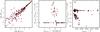 |
Fig. 1 Comparison of Xe vi data given by Biémont et al. (2005, B+05) and Gallardo et al. (2015, G+15). Left: weighted oscillator strengths (log gf) in G+15 as a function of the B+05 values, middle: ratio of atomic level energies as a function of the B+05 values, right: ratio of line wavelengths as a function of the B+05 values. |
3. Model atmospheres
Our model atmospheres are plane-parallel, chemically homogeneous, and in hydrostatic and radiative equilibrium. They are calculated with the Tübingen NLTE Model Atmosphere Package (TMAP4, Werner et al. 2003, 2012a). Model atoms were constructed from the Tübingen Model Atom Database (TMAD5, Rauch & Deetjen 2003). TMAD has been constructed as part of the Tübingen contribution to the German Astrophysical Virtual Observatory (GAVO6).
4. Xe vi transition probabilities
For their analysis of RE 0503−289, Werner et al. (2012b) used Xe vi data of Reyna Almandos et al. (2001), who used the Hartree-Fock relativistic (HFR) approach to calculate weighted oscillator strengths (gf) of 104 spectral lines belonging to the 5s5p2, 5s25d, 5s26s, 5s5p5d, 5p3, and 5s5p6s transitions array. In addition, gf-values of an experimental and theoretical study by Biémont et al. (2005) were used. These replaced gf-values of Reyna Almandos et al. (2001) where available. They were calculated for Δn = 0 and Δn = 1 transitions connecting the 5s2nl [np (n = 5–8); nf (n = 4–5); nh (n = 6–8); nk (n = 8)], 5s5pnl (nl = 5d,6s), 5p3, 5s2nl [ns (n = 6–8); nd (n = 5–8); ng (n = 5–6); ni (n = 7–8)], and 5s5p2 configurations. Core-polarization (CP) effects were included in their HFR approach. Good agreement was observed between theory and experiment.
Gallardo et al. (2015) observed 243 lines (146 classified for the first time) of the Xe vi spectrum within 400 Å ≤ λ ≤ 5500 Å. They calculated gf-values of 5s5p5d and 5s5p6s configurations. Biémont et al. (2005) encountered a problem in matching the 6d experimental level in their least-squares calculations, which Gallardo et al. (2015, see this paper for further technical details) solved by adjusting configuration interaction (CI) integrals. They achieved standard deviations of 149 cm-1 in the odd parity energies (35 configurations) and 154 cm-1 (34 configurations) in the even parity.
We updated our Xe vi model ion (Werner et al. 2012b) with their experimental level energies (88 levels, 32 classified for the first time, 33 with revised energies) and oscillator strengths (used in the formulae for the cross-sections of radiative and collisional bound-bound transitions). The new Xe vi model ion is available via TMAD.
Figure 1 shows the comparison of the Xe vi log gf values, level energies, and line wavelengths of Biémont et al. (2005) and the Gallardo et al. (2015). For the strongest lines, that is, log gf> 0.0, the agreement of the oscillator strengths is very good. The energy levels deviate significantly in the 230 000 cm-1<E< 350 000 cm-1 interval. This results in stronger differences of the lines’ wavelengths in the ultraviolet wavelength range (λ< 1700 Å). The following comparison will verify the quality of the new data.
We start reproducing the lines shown by Werner et al. (2012b). Table 1 shows a comparison of the log gf values that they used with the new values.
Figure 2 demonstrates how the new oscillator strengths influence the line-profile fits. Because of their much higher log gf values, Xe viλλ 928.366,1101.947 Å now match the observation significantly better, while the other lines are almost unchanged. The Xe vii lines are too strong, most likely as a result of our insufficient Xe vii model ion, for which only two oscillator strengths are known (namely of these two lines). In Sect. 5, we search in the FUSE and HST/STIS spectra for further Xe vi lines to evaluate the oscillator strengths.
Comparison of the log gf values of Xe vi lines calculated by Biémont et al. (2005) and used by Werner et al. (2012b) with those calculated by Gallardo et al. (2015).
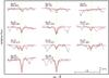 |
Fig. 2 Xe vi and Xe vii lines calculated from TMAP model atmospheres with , log g = 7.5, and log Xe = −4.2 (mass fraction) compared with the FUSE observation. Thin (blue in the online version): model of Werner et al. (2012b, N ivλ 1136.27 Å, thick (red) our model. The vertical bar indicates 10 % of the continuum flux level. |
5. Line identification and abundance determination
We compared our best model spectra with our FUSE and STIS observations to identify additional Xe vi lines. We found only a few (Fig. 3). Xe viλλ 929.121,1017,270 Å have apparently blends with so far unknown lines. Xe viλ 1298.910 Å matches the STIS observation well. Since all observed Xe lines are reproduced well, we confirm the abundance determination by Werner et al. (2012b, log Xe = −4.2 ± 0.6. The two identified Xe viiλλ 995.511,1077.12 Å lines (oscillator strengths from Kernahan et al. 1980; Biémont et al. 2007, respectively) are stronger than observed at this abundance (hence the relatively broad error range), but this may be an artifact due to the lack of reliable Xe vii oscillator strengths, cf. Werner et al. (2012b, see Sect. 1.
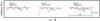 |
Fig. 3 Xe vi lines calculated from the same models as in Fig. 2 compared with the FUSE and STIS (right panel, Ni vλ 1298.738 Å appears left of Xe viiλ 1298.910 Å) observations. Thin (blue in the online version): model without Xe, thick (red) model including Xe. |
6. Results and conclusions
The recently presented oscillator strengths of Gallardo et al. (2015, 243 lines) complement and improve available data of Reyna Almandos et al. (2001, 104 lines) and Biémont et al. (2005, 491 lines). A comparison of data for lines that are listed in Gallardo et al. (2015) and Biémont et al. (2005) showed that the log gf values agree well for the strongest lines. Deviations in the line wavelengths are noted, but they do not affect the identified lines in the UV spectra of RE 0503−289 and cannot be
assessed. However, a comprehensive recalculation of Xe vi transition probabilities is desirable.
The oscillator strengths of Gallardo et al. (2015) significantly improve the agreement of the synthetic Xe vi line profiles with the observations in two of nine cases. The abundance determination of Werner et al. (2012b, log Xe = −4.2±0.6 was confirmed.
Figure 4 shows that Xe vii is the dominant Xe ionization stage in the in the line-forming region (−4 ≲ log m ≲ 0.5). m is the mass column density, measured from the outer limit of the atmosphere. Therefore, we expect to identify many more Xe vii lines once reliable oscillator strengths for the complete Xe vii model ion are available. This is mandatory to be able to reduce the uncertainty in the Xe abundance analysis.
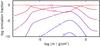 |
Fig. 4 Xe vi ionization fractions in our best model for RE 0503−289 (Rauch et al. 2015). |
Acknowledgments
T.R. and D.H. are supported by the German Aerospace Center (DLR, grants 05 OR 1402 and 50 OR 1501, respectively). The GAVO project at Tübingen had been supported by the Federal Ministry of Education and Research (BMBF, grants 05 AC 6 VTB, 05 AC 11 VTB). Financial support from the Belgian FRS-FNRS is also acknowledged. P.Q. is research director of this organization. Some of the data presented in this paper were obtained from the Mikulski Archive for Space Telescopes (MAST). STScI is operated by the Association of Universities for Research in Astronomy, Inc., under NASA contract NAS5-26555. Support for MAST for non-HST data is provided by the NASA Office of Space Science via grant NNX09AF08G and by other grants and contracts. This research has made use of NASA’s Astrophysics Data System and the SIMBAD database, operated at CDS, Strasbourg, France.
References
- Biémont, É., Buchard, V., Garnir, H.-P., Lefèbvre, P.-H., & Quinet, P. 2005, Eur. Phys. J. D, 33, 181 [NASA ADS] [CrossRef] [EDP Sciences] [Google Scholar]
- Biémont, É., Clar, M., Fivet, V., et al. 2007, Eur. Phys. J. D, 44, 23 [NASA ADS] [CrossRef] [EDP Sciences] [Google Scholar]
- Gallardo, M., Raineri, M., Reyna Almandos, J., Pagan, C. J. B., & Abrahão, R. A. 2015, ApJS, 216, 11 [NASA ADS] [CrossRef] [Google Scholar]
- Kernahan, J. A., Pinnington, E. H., O’Neill, J. A., Bahr, J. L., & Donnelly, K. E. 1980, J. Opt. Soc. Am. (1917−1983), 70, 1126 [NASA ADS] [CrossRef] [Google Scholar]
- Rauch, T., & Deetjen, J. L. 2003, in Stellar Atmosphere Modeling, eds. I. Hubeny, D. Mihalas, & K. Werner, ASP Conf. Ser., 288, 103 [Google Scholar]
- Rauch, T., Werner, K., Biémont, É., Quinet, P., & Kruk, J. W. 2012, A&A, 546, A55 [NASA ADS] [CrossRef] [EDP Sciences] [Google Scholar]
- Rauch, T., Werner, K., Quinet, P., & Kruk, J. W. 2014a, A&A, 564, A41 [NASA ADS] [CrossRef] [EDP Sciences] [Google Scholar]
- Rauch, T., Werner, K., Quinet, P., & Kruk, J. W. 2014b, A&A, 566, A10 [NASA ADS] [CrossRef] [EDP Sciences] [Google Scholar]
- Rauch, T., Werner, K., Quinet, P., & Kruk, J. W. 2015, A&A, 577, A6 [NASA ADS] [CrossRef] [EDP Sciences] [Google Scholar]
- Reyna Almandos, J., Sarmiento, R., Raineri, M., Bredice, F., & Gallardo, M. 2001, J. Quant. Spec. Radiat. Transf., 70, 189 [NASA ADS] [CrossRef] [Google Scholar]
- Werner, K., Deetjen, J. L., Dreizler, S., et al. 2003, in Stellar Atmosphere Modeling, eds. I. Hubeny, D. Mihalas, & K. Werner, ASP Conf. Ser., 288, 31 [Google Scholar]
- Werner, K., Dreizler, S., & Rauch, T. 2012a, TMAP: Tübingen NLTE Model-Atmosphere Package, Astrophysics Source Code Library [Google Scholar]
- Werner, K., Rauch, T., Ringat, E., & Kruk, J. W. 2012b, ApJ, 753, L7 [NASA ADS] [CrossRef] [Google Scholar]
All Tables
Comparison of the log gf values of Xe vi lines calculated by Biémont et al. (2005) and used by Werner et al. (2012b) with those calculated by Gallardo et al. (2015).
All Figures
|
Fig. 1 Comparison of Xe vi data given by Biémont et al. (2005, B+05) and Gallardo et al. (2015, G+15). Left: weighted oscillator strengths (log gf) in G+15 as a function of the B+05 values, middle: ratio of atomic level energies as a function of the B+05 values, right: ratio of line wavelengths as a function of the B+05 values. |
| In the text | |
|
Fig. 2 Xe vi and Xe vii lines calculated from TMAP model atmospheres with , log g = 7.5, and log Xe = −4.2 (mass fraction) compared with the FUSE observation. Thin (blue in the online version): model of Werner et al. (2012b, N ivλ 1136.27 Å, thick (red) our model. The vertical bar indicates 10 % of the continuum flux level. |
| In the text | |
|
Fig. 3 Xe vi lines calculated from the same models as in Fig. 2 compared with the FUSE and STIS (right panel, Ni vλ 1298.738 Å appears left of Xe viiλ 1298.910 Å) observations. Thin (blue in the online version): model without Xe, thick (red) model including Xe. |
| In the text | |
|
Fig. 4 Xe vi ionization fractions in our best model for RE 0503−289 (Rauch et al. 2015). |
| In the text | |
Current usage metrics show cumulative count of Article Views (full-text article views including HTML views, PDF and ePub downloads, according to the available data) and Abstracts Views on Vision4Press platform.
Data correspond to usage on the plateform after 2015. The current usage metrics is available 48-96 hours after online publication and is updated daily on week days.
Initial download of the metrics may take a while.