| Issue |
A&A
Volume 577, May 2015
|
|
|---|---|---|
| Article Number | A42 | |
| Number of page(s) | 6 | |
| Section | Stellar structure and evolution | |
| DOI | https://doi.org/10.1051/0004-6361/201425481 | |
| Published online | 29 April 2015 | |
New evolutionary models for pre-main sequence and main sequence low-mass stars down to the hydrogen-burning limit
1
University of Exeter, Physics and Astronomy, EX4 4,
QL Exeter
UK
e-mail:
This email address is being protected from spambots. You need JavaScript enabled to view it.
2
École Normale Supérieure, Lyon, CRAL (UMR CNRS 5574), Université
de Lyon, 69364
Lyon Cedex 07,
France
e-mail: This email address is being protected from spambots. You need JavaScript enabled to view it.
; This email address is being protected from spambots. You need JavaScript enabled to view it.
; This email address is being protected from spambots. You need JavaScript enabled to view it.
Received: 8 December 2014
Accepted: 24 February 2015
Abstract
We present new models for low-mass stars down to the hydrogen-burning limit that consistently couple atmosphere and interior structures, thereby superseding the widely used BCAH98 models. The new models include updated molecular linelists and solar abundances, as well as atmospheric convection parameters calibrated on 2D/3D radiative hydrodynamics simulations. Comparison of these models with observations in various colour-magnitude diagrams for various ages shows significant improvement over previous generations of models. The new models can solve flaws that are present in the previous ones, such as the prediction of optical colours that are too blue compared to M dwarf observations. They can also reproduce the four components of the young quadruple system LkCa 3 in a colour–magnitude diagram with one single isochrone, in contrast to any presently existing model. In this paper we also highlight the need for consistency when comparing models and observations, with the necessity of using evolutionary models and colours based on the same atmospheric structures.
Key words: stars: evolution / stars: low-mass / stars: pre-main sequence / Hertzsprung-Russell and C-M diagrams / convection
© ESO, 2015
1. Introduction
In 1998, our team released a set of evolutionary models for low-mass stars (Baraffe et al. 1998, hereafter BCAH98) based on the so-called NextGen atmosphere models (Hauschildt et al. 1999) that marked a new era of models that consistently coupled interior and atmosphere structures. These models became very popular because they successfully reproduce various observational constraints, such as mass-luminosity and mass-radius relationships and colour-magnitude diagrams. The models, however, had some important shortcomings, such as predicting optical (V − I) colours that are too blue for a given magnitude (see Sect. 3.1). Later generations of models included improved molecular linelists for various atmospheric absorbers, such as the AMES linelists used in the Dusty and Cond models (Chabrier et al. 2000; Allard et al. 2001; Baraffe et al. 2003), but they still show shortcomings (see Sect. 3.2). After a long effort to solve these flaws, efforts have paid off with the release of current models that supersede the BCAH98 models. In this paper, we describe the main physical ingredients of the models and compare them to a selection of observations that highlight the improvement of these new models over previous ones.
2. Model description
Evolutionary calculations are based on the same input physics describing stellar and substellar interior structures as are used in Chabrier & Baraffe (1997) and Baraffe et al. (1998). The major changes concern the atmosphere models, which provide the outer boundary conditions for the interior structure calculation, and the colours and magnitudes for a given star mass at any given age. Substantial changes have been made since the NextGen atmosphere models used in the BCAH98 evolutionary models. A preliminary set of atmosphere models, referred to as the BT-Settl models (Allard et al. 2012a,b; Rajpurohit et al. 2013), include some of these changes, which are briefly summarised below. More recent modifications concerning the treatment of convection are described in Sect. 2.3.
2.1. Molecular linelists and cloud formation
Line opacities for several important molecules have been updated, notably the water linelist from Barber et al. (2006), metal hydrides such as CaH, FeH, CrH, TiH from Bernath (2006), vanadium oxide from Plez (2004, priv. comm.), and carbon dioxide from Tashkun et al. (2004). For TiO, the present set of atmosphere models uses the linelist from Plez (1998). This list is not as complete at high energies as the AMES linelist (Schwenke 1998) adopted in Allard et al. (2001, 2012a), with only 11 × 106 lines compared to the 160 × 106 of Schwenke (1998). But the Plez linelist reproduces the overall band strengths better and thus generally improves the optical colours (Fig. 4). Obviously, the field is still in need of a new, complete, and accurate theoretical TiO linelist to allow quantitative high-resolution spectroscopic analysis of this important molecule, as recently pointed by the high-resolution transmission spectrum analysis of a transiting exoplanet (Hoeijmakers et al. 2015).
Condensation of up to 200 types of liquids and solids is included in the atmospheric equation of state. The formation and sedimentation of clouds and depletion of condensible material is treated in the self-consistent timescale approach of Allard et al. (2012a). They used a monodisperse grain size distribution for each cloud layer, but current version of the models now considers a log-normal distribution over 1.8 decades in size in 12 bins with the altitude-dependent size determined by the same timescale formalism as in Allard et al. (2012a). The set of 60 grain types included in calculating the cloud opacity has also been updated with the optical data for several low-temperature condensates, which become important in the atmospheres of T dwarfs, which are not discussed in this paper (Homeier et al., in prep.).
2.2. Solar abundances
Solar abundances have been revised over the past decade based on radiation hydrodynamical simulations of the solar photosphere combined with 3D non-local thermodynamical equilibrium radiative transfer (Asplund et al. 2009; Caffau et al. 2011). This leads to a substantial reduction of carbon, nitrogen, and oxygen abundances compared to the abundances of Grevesse et al. (1993), previously used in the NextGen and AMES-Dusty/Cond models. The present models adopt the solar composition of Asplund et al. (2009) with revisions of the elemental abundances of C, N, O, Ne, P, S, K, Fe, Eu, Hf, Os, and Th obtained by the CIFIST project (Caffau et al. 2011). This yields, in particular, a slight upward revision of carbon, nitrogen, and oxygen abundances and an increased total heavy element fraction by mass, with Z = 0.0153 compared to 0.0122 in Asplund et al. (2005) and 0.0134 in Asplund et al. (2009). Although the individual differences with the Asplund et al. (2009) elemental abundances are modest, Antia & Basu (2011) and Basu & Antia (2013) have found that the higher overall metal content of the CIFIST abundances is in better agreement with helioseismology results for the solar interior. The helium abundance adopted in the atmosphere models is fixed to Yini = 0.271, which is representative of the initial solar helium abundance (Serenelli & Basu 2010; Basu & Antia 2013).
2.3. Treatment of convection
Radiative-convective equilibrium in the PHOENIX atmosphere models is calculated using the mixing length theory (or MLT, see Kippenhahn & Weigert 1990). The main free parameter within this framework is the mixing length lmix, expressed in terms of the pressure scale height HP and lmix describes the efficiency of the convective energy transport in terms of the superadiabaticity of the temperature gradient. All previous PHOENIX models have used a constant value for  :
:  in the NextGen and Cond/Dusty models and
  in Allard et al. (2012a).
In the present work, the determination of  is inspired by the work of Ludwig et al. (1999, 2002). It is based on comparisons between 1D MLT models and 2D/3D RHD simulations that cover main sequence and pre-MS models down to the hydrogen-burning limit and below (Freytag et al. 2010, 2012). Since the RHD models include a basic treatment of dust formation, they also allow the calibration of late M dwarfs, where cloud opacity is becoming relevant. This calibration yields a value of
  for the Sun. The value of increases for later type stars, up to values ≳2 × HP for the coolest and densest models (Teff< 3000 K and log g> 4.5). Comparisons between 1D and RHD pressure-temperature profiles are shown in Fig. 1. The adopted value of , for a given Teff and log g, provides the best overall agreement that can be obtained; however, the agreement is not perfect all the way from the top to the bottom of the atmosphere, reflecting limitations in the MLT formalism for properly handling atmospheric convection (Homeier et al., in prep.).
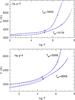 |
Fig. 1 Comparisons of pressure-temperature atmospheric profiles between present 1D (solid blue) and CO5BOLD RHD (dash-dot black) models, for different effective temperatures and surface gravities, as indicated in the panels for each curves. Pressure unit is dyne/cm-2. Calibration of lmix based on such comparisons yields |


2.4. Evolutionary models
Current models cover the evolution of pre-MS and MS stars from 0.07 M⊙ to 1.4 M⊙. Calibration of a 1 M⊙ star sequence to fit the fundamental parameters of the Sun (R⊙, L⊙) at its age requires a value for the interior structure of the mixing length  and a helium abundance Y = 0.28. We used this value of helium for the complete grid of evolutionary models. The value adopted in the atmosphere models is slightly different (Y = 0.271, see Sect. 2.2). To appreciate the effect of this inconsistency, we have recalculated a full grid of evolutionary models assuming the same He abundance Y = 0.271 in the interior structure as in the atmosphere models. The effect of such a variation in Y on Teff for the whole range of masses considered is less than 1%. The maximum effect on the luminosity is found for the highest masses (M ≳ 1 M⊙) and reaches at most 10%. For a 1 M⊙ star, the effect on the luminosity is less than 5% for ages ≲2 Gyr, and up to 10% for ages ≳ 2 Gyr. We have also computed a few atmosphere models again with Y = 0.28 for a range of Teff between 2600 K and 6000 K and of gravities log g between 3.5 and 5. The effect of such a variation in Y is negligible on the atmospheric thermal profiles (less than a 1% effect on the pressure at a given temperature) and on the photometry (differences less than 0.01 mag for all colours explored).
We fixed  for the complete grid of evolutionary models for the interior structure. A fully consistent approach would be to adopt the value obtained for the corresponding atmosphere model, i.e
  . We checked that this is unnecessary. Indeed, values of only start to depart significantly from 1.6 × HP for the coolest and densest models (Teff< 3000 K and log g> 4.5), reaching values up to 2 × HP or more. This concerns masses <0.2 M⊙, where a variation of
  between 1.6 × HP and 2 × HP has an insignificant effect on the evolution.
As illustrated in Fig. 2, the new models predict different positions of isochrones than do the BCAH98 models. Below Teff ≲ 2800 K, dust starts to form in the upper atmosphere and affects atmospheric thermal profiles and spectra. In the current grid of evolutionary models with Teff> 2000 K, the effects of cloud opacity only gradually become visible for the latest M and early L dwarfs (Teff ≲ 2500 K). They are becoming crucial for models of L and T dwarfs, which will be examined in a forthcoming study.
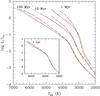 |
Fig. 2 Comparison of present models with the BCAH98 models for various isochrones, as indicated in the figure and inset. Solid (red): present models; long dash (black): BCAH98 models with |
Theoretical mass-radius relationships for 0.1 Gyr and 1 Gyr are shown in Fig. 3 for different sets of models. As shown in Chabrier & Baraffe (1997), the mass-radius relationship for low-mass stars is essentially fixed by the equation of state, with a very small dependence on the atmosphere treatment. The differences between present models and the BCAH98 models essentially stem from the different values of the interior mixing length  used. As shown in Fig. 3, the effect of the interior He abundance Yint slightly affects the mass-radius relationship for masses ≳1 M⊙.
 |
Fig. 3 Comparison of theoretical mass-radius relationships for ages of 0.1 Gyr (upper panel) and 1 Gyr (lower panel) and based on different sets of models: present models with Yint = 0.28 (solid red) and Yint = 0.271 (short-dash red); BCAH98 models with |
3. Comparison with observations
In this section, we highlight the significant improvement provided by this new set of models, which solve some of the problems of the BCAH98 models, through a selection of observational tests. Colour−magnitude diagrams (CMDs) provide the best validity test, as they test the consistency between interior and atmosphere structures.
3.1. Optical colours
As mentioned in the introduction, a well-known flaw of the BCAH98 models is the prediction of colours that are too blue (V − I). Figure 4 compares models at 1 Gyr with solar-neighbourhood and disk objects with parallax (Monet et al. 1992; Leggett 1992; Cantrell et al. 2013). The comparison shows that this persistent problem of the models seems to be solved by several improvements. The most important one is the use of the TiO linelist from Plez (1998). The impact of the TiO linelist has already been noticed with the generation of models following the NextGen ones, such as the Dusty models (Chabrier et al. 2000; Allard et al. 2001). The former ones use the linelist by Jorgensen (1994), while the latter ones include the AMES TiO linelist of Schwenke (1998). The improvement in () colours of models that include the AMES TiO linelist of Schwenke (1998) was significant (see Fig. 4), but still unable to yield satisfactory agreement with observations. Indeed, an offset in () colours of ~0.4 mag remained between Teff ~ 3600 K (MV ~ 10) and Teff ~ 2300 K (MV ~ 19, see Chabrier et al. 2000). Improvement due to the implementation of the Plez (1998) TiO linelist in the new models is illustrated in Fig. 4 by the comparison between present models (TiOPl) and the same models based on the AMES TiO linelist (TiOAM).
 |
Fig. 4 Comparison of 1 Gyr isochrones with disk dwarfs in an optical CMD. Present models based on the Plez TiO (solid red) and the AMES TiO (dash red) linelists are shown, along with the BCAH98 models (long dash black). The magenta open circles are disk objects with parallax (Monet et al. 1992; Leggett 1992) and the blue squares are from the recent 5 pc and 10 pc solar neighbourhood samples of Cantrell et al. (2013) with more accurate parallaxes and cleaned of binary systems. The numbers close to the red open circles on the solid curve give Teff and mass (in M⊙ in the brackets) for selected models. |
Another positive effect stems from the change in solar abundances, with a decrease in oxygen abundance by ~22% between the Grevesse et al. (1993), used in previous sets of models, and the presently used Caffau et al. (2011) abundances. As a consequence of relatively less O, the flux in the IR generally increases owing to weaker water absorption. Because of flux redistribution, the flux in the V-band decreases relative to the flux at longer wavelengths. This is an important effect, illustrating how water abundance affects optical colours due to flux redistribution.
 |
Fig. 5 Comparison of 1 Gyr isochrones with disk dwarfs in near-IR CMDs in CIT filters. Solid (red): new models; long dash (black): BCAH98 models with |
3.2. Near-infrared colours
The new models yield also a significantly better match with observations for relatively old objects (age ≳1 Gyr, log g ≳ 4.5) in near-IR CMDs, as illustrated in Fig. 5. This stems from the use of the more complete and accurate water linelist of Barber et al. (2006), compared to previously used ones, namely Miller et al. (1994) in NextGen and Partridge & Schwenke (1997) in Dusty/Cond.
To illustrate the impact of the new models at low gravities and in a similar range of effective temperatures (Teff> 2000 K), we also compared them to data in the young cluster σ Orionis (Peña Ramírez et al. 2012), with an age of a few Myr (log g ≲ 4). The results are shown in Fig. 6 in various CMDs. Fluxes from the models have been transformed in the VISTA filters to be consistent with the data of Peña Ramírez et al. (2012). Comparison of models in CMDs (or luminosity-Teff diagrams) with observations in young clusters and star formation regions should always be taken with caution owing to the observed luminosity spread and the effect of initial conditions and accretion history (Baraffe et al. 2002, 2009, 2012). The comparison in Fig. 6, however, is illustrative of the overall improvement in ZJHK filters of the new models compared to the BCAH98 ones. The latter indeed provide poor agreement with observations at young ages in near-IR CMDs, as illustrated in Fig. 6. For this reason, models had to be compared with data in L − Teff or HR diagrams, which implied the use of very uncertain bolometric corrections and spectral type-Teff or colour-Teff scales. The agreement of the new models with observations, however, deteriorates at the faintest magnitudes by up to ~ 0.1 mag in () and ~0.4 mag in (). Given photometric uncertainties and possible K-band excess at this age owing to the presence of a circumstellar disk, it is premature to draw any conclusion on the reason for these discrepancies.
 |
Fig. 6 Comparison of models with observations in σ Orionis in various CMDs (VISTA filters). Isochrones of 1 Myr and 10 Myr are displayed for various sets of models: present models (red): solid (1 Myr) and dash-dot (10 Myr). BCAH98 models with |
3.3. Multiple systems
Stringent tests of evolutionary models are provided by coeval multiple systems. The recent discovery of the quadruple pre-main sequence system LkCa 3 is interesting in this respect (Torres et al. 2013). If one admits that the four components of LkCa 3 should be coeval and must lie on the same isochrone, they make an excellent test of evolutionary models. This supposes that early history of accretion has not altered their structure (Baraffe et al. 2009, 2012) and that their position in a CMD or L − Teff diagram can be reproduced by non-accreting evolutionary models.
With this assumption, Torres et al. (2013) find that no currently available model is able to reproduce the position of the four components with one single isochrone in a CMD. In contrast, our new models do fulfil this stringent constraint within the error bars (see Fig. 7). The new models agree with observations for an age of 1.6 Myr. In comparison, the best-fit 6.3 Myr isochrone of the BCAH98 models with  is unable to match the coolest component LkCa 3 Ab, which can be fitted by an isochrone of 2.5 Myr. A similar problem arises with the BCAH98 models using
  . The same failure was reported by Torres et al. (2013, see their Fig. 6) with the Dartmouth models (Dotter et al. 2008).
As a final note, even if accretion history can have an impact on the structure of young objects, as suggested by Baraffe et al. (2012), this does not necessarily affect all objects in the same way. Even for binary or multiple systems, each component has its own accretion history, and its structure may be differently altered by accretion, since the effect depends on the total amount of accreted mass (see Baraffe et al. 2012 for details). Disentangling the remaining uncertainties of models and possible effects of accretion when comparing models to young multiple systems is thus not straightforward. We hope that many more such multiple systems, spanning a wide range of masses and ages, will be discovered in the near future to provide more clues to the remaining model uncertainties (e.g. convection treatment, opacity uncertainty) and/or to the impact of accretion for the youngest systems.
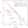 |
Fig. 7 Comparison of models with the four components of the quadruple system LkCa 3 (Torres et al. 2013). The best-fit isochrone is shown for various sets of models. Present models for an age of 1.6 Myr (solid red). BCAH98 models with |
3.4. Tests of stellar evolutionary models
For the sake of testing evolutionary models against observations, it is crucial to use the synthetic colours and magnitudes predicted by the same atmosphere models as those that provide the outer boundary conditions for the interior structure. Using “hybrid” models, based on atmospheric thermal profiles for the interior structure from one set of atmosphere models and colours/magnitudes from another set, yields incorrect results. Figure 8 illustrates this point, showing in two CMDs for various isochrones a comparison between the present set of models, the BCAH98 models, and a hybrid model based on BCAH98 evolutionary models (relying on the NextGen atmosphere models) and the colours and magnitudes from current atmosphere models. The positions and slopes of the hybrid model isochrones are significantly different from both the new and the BCAH98 models. Using these and similar hybrid models to derive cluster ages and masses or to test them against multiple systems yields incorrect results and incorrect conclusions on the validity or invalidity of the models. Such comparisons, often seen in the literature, are totally meaningless.
 |
Fig. 8 Comparison of 10 Myr and 1 Gyr isochrones for various sets of models in two CMDs. Solid (red): present models. Long dash (black): BCAH98 models with |
4. Conclusions
The new set of evolutionary models presented in this paper, consistently coupling internal and atmospheric structures, show significant improvement over previous generations. They solve some of the persistent flaws present in them, such as predicting optical colours that are too blue. Significant improvement in the atmosphere models, in terms of updated molecular linelists and revised solar abundances, provide a much better match to observations. More systematic tests of current models against observations will help to identify the remaining uncertainties. The calibration of the mixing-length parameter, as presented in this work, provides overall good agreement between 1D and multi-D RHD thermal profiles. This exercise highlights the poor approximation of using a constant value for for pre-main sequence and main-sequence low-mass stars. The agreement, however, is not perfect, depending on the effective temperature and the surface gravity. This very likely reflects the limitation of the MLT formalism to correctly capture the thermal properties of convectively unstable atmospheres over a wide range of parameters. We note as well that remaining uncertainties in the multi-D RHD simulations are not excluded. Efforts towards developing such simulations in cool atmospheres need to be pursued. Since models at young ages are particularly sensitive to the treatment of atmospheric convection (Baraffe et al. 2002), comparisons between models and observations of objects in young clusters (age ≲10 Myr) will help to improve the treatment of convection.
Following the release of these new models down to the hydrogen-burning limit1, we are currently working on their extension to L, T, and Y dwarfs, including dust formation and settling. This will provide a complete and coherent set of models for low-mass stars and brown dwarfs down to Jupiter-mass objects.
Isochrones are available at: http://emps.exeter.ac.uk/physics-astronomy/staff/ib233 or http://perso.ens-lyon.fr/isabelle.baraffe/BHAC15dir
Acknowledgments
This work is supported by Royal Society award WM090065. It is also partly supported by the ERC under the European Community’s Seventh Framework Programme (FP7/2007−2013 Grant Agreement No. 247060), the consolidated STFC grant ST/J001627/1, the French ANR through the GuEPARD project grant ANR10-BLANC0504-01, and the PNPS of the CNRS (INSU). We thank the CHARA team (Russel White, Todd Henry, Cassy Davidson, Justin Cantrell) for providing the CHARA data and Guillermo Torres for providing information on LkCa 3. We thank José Caballero for discussion and Richard Freedman and Jonathan Tennyson for sharing their insights into the status of molecular line data. The model atmospheres used in this study were calculated at the PSMN of the ENS-Lyon and at the GWDG in co-operation with the Institut für Astrophysik Göttingen.
References
- Allard, F., Hauschildt, P. H., Alexander, D. R., Tamanai, A., & Schweitzer, A. 2001, ApJ, 556, 357 [NASA ADS] [CrossRef] [Google Scholar]
- Allard, F., Homeier, D., & Freytag, B. 2012a, Roy. Soc. London Philos. Trans. Ser. A, 370, 2765 [Google Scholar]
- Allard, F., Homeier, D., Freytag, B., & Sharp, C. M. 2012b, in EAS Pub. Ser. 57, eds. C. Reylé, C. Charbonnel, & M. Schultheis, 3 [Google Scholar]
- Antia, H. M., & Basu, S. 2011, J. Phys. Conf. Ser., 271, 012034 [NASA ADS] [CrossRef] [Google Scholar]
- Asplund, M., Grevesse, N., & Sauval, A. J. 2005, in Cosmic Abundances as Records of Stellar Evolution and Nucleosynthesis, ASP Conf. Ser., 336, 25 [Google Scholar]
- Asplund, M., Grevesse, N., Sauval, A. J., & Scott, P. 2009, ARA&A, 47, 481 [NASA ADS] [CrossRef] [Google Scholar]
- Baraffe, I., Chabrier, G., Allard, F., & Hauschildt, P. H. 1998, A&A, 337, 403 [NASA ADS] [Google Scholar]
- Baraffe, I., Chabrier, G., Allard, F., & Hauschildt, P. H. 2002, A&A, 382, 563 [NASA ADS] [CrossRef] [EDP Sciences] [Google Scholar]
- Baraffe, I., Chabrier, G., Barman, T. S., Allard, F., & Hauschildt, P. H. 2003, A&A, 402, 701 [NASA ADS] [CrossRef] [EDP Sciences] [Google Scholar]
- Baraffe, I., Chabrier, G., & Gallardo, J. 2009, ApJ, 702, L27 [NASA ADS] [CrossRef] [Google Scholar]
- Baraffe, I., Vorobyov, E., & Chabrier, G. 2012, ApJ, 756, 118 [NASA ADS] [CrossRef] [Google Scholar]
- Barber, R. J., Tennyson, J., Harris, G. J., & Tolchenov, R. N. 2006, MNRAS, 368, 1087 [NASA ADS] [CrossRef] [Google Scholar]
- Basu, S., & Antia, H. M. 2013, J. Phys. Conf. Ser., 440, 012017 [NASA ADS] [CrossRef] [Google Scholar]
- Bernath, P. 2006, in Astrochemistry – From Laboratory Studies to Astronomical Observations, eds. R. I. Kaiser, P. Bernath, Y. Osamura, S. Petrie, & A. M. Mebel, AIP Conf. Ser., 855, 143 [Google Scholar]
- Caffau, E., Ludwig, H.-G., Steffen, M., Freytag, B., & Bonifacio, P. 2011, Sol. Phys., 268, 255 [NASA ADS] [CrossRef] [Google Scholar]
- Cantrell, J. R., Henry, T. J., & White, R. J. 2013, AJ, 146, 99 [NASA ADS] [CrossRef] [Google Scholar]
- Chabrier, G., & Baraffe, I. 1997, A&A, 327, 1039 [NASA ADS] [Google Scholar]
- Chabrier, G., Baraffe, I., Allard, F., & Hauschildt, P. 2000, ApJ, 542, 464 [NASA ADS] [CrossRef] [Google Scholar]
- Dotter, A., Chaboyer, B., Jevremović, D., et al. 2008, ApJS, 178, 89 [NASA ADS] [CrossRef] [Google Scholar]
- Freytag, B., Allard, F., Ludwig, H.-G., Homeier, D., & Steffen, M. 2010, A&A, 513, A19 [NASA ADS] [CrossRef] [EDP Sciences] [Google Scholar]
- Freytag, B., Steffen, M., Ludwig, H.-G., et al. 2012, J. Comput. Phys., 231, 919 [Google Scholar]
- Grevesse, N., Noels, A., & Sauval, A. J. 1993, A&A, 271, 587 [NASA ADS] [Google Scholar]
- Hauschildt, P. H., Allard, F., Ferguson, J., Baron, E., & Alexander, D. R. 1999, ApJ, 525, 871 [NASA ADS] [CrossRef] [Google Scholar]
- Hoeijmakers, H. J., de Kok, R. J., Snellen, I. A. G., et al. 2015, A&A, 575, A20 [NASA ADS] [CrossRef] [EDP Sciences] [Google Scholar]
- Jorgensen, U. G. 1994, A&A, 284, 179 [NASA ADS] [Google Scholar]
- Kippenhahn, R., & Weigert, A. 1990, Stellar Structure and Evolution (Berlin, Heidelberg, New York: Springer Astron. Astrophys. Lib.) [Google Scholar]
- Leggett, S. K. 1992, ApJS, 82, 351 [NASA ADS] [CrossRef] [Google Scholar]
- Ludwig, H.-G., Freytag, B., & Steffen, M. 1999, A&A, 346, 111 [NASA ADS] [Google Scholar]
- Ludwig, H.-G., Allard, F., & Hauschildt, P. H. 2002, A&A, 395, 99 [NASA ADS] [CrossRef] [EDP Sciences] [Google Scholar]
- Miller, S., Tennyson, J., Jones, H. R. A., & Longmore, A. J. 1994, in Molecules in the Stellar Environment (Berlin: Springer Verlag), ed. U. G. Jorgensen, IAU Colloq. 146, Lect. Notes Phys., 428, 296 [Google Scholar]
- Monet, D. G., Dahn, C. C., Vrba, F. J., et al. 1992, AJ, 103, 638 [NASA ADS] [CrossRef] [Google Scholar]
- Partridge, H., & Schwenke, D. W. 1997, J. Chem. Phys., 106, 4618 [NASA ADS] [CrossRef] [Google Scholar]
- Peña Ramírez, K., Béjar, V. J. S., Zapatero Osorio, M. R., Petr-Gotzens, M. G., & Martín, E. L. 2012, ApJ, 754, 30 [NASA ADS] [CrossRef] [Google Scholar]
- Plez, B. 1998, A&A, 337, 495 [NASA ADS] [Google Scholar]
- Rajpurohit, A. S., Reylé, C., Allard, F., et al. 2013, A&A, 556, A15 [NASA ADS] [CrossRef] [EDP Sciences] [Google Scholar]
- Schwenke, D. W. 1998, Faraday Discussions, 109, 321 [NASA ADS] [CrossRef] [Google Scholar]
- Serenelli, A. M., & Basu, S. 2010, ApJ, 719, 865 [NASA ADS] [CrossRef] [Google Scholar]
- Tashkun, S. A., Perevalov, V. I., Teffo, J.-L., et al. 2004, in SPIE Conf. Ser. 5311, eds. L. N. Sinitsa, & S. N. Mikhailenko, 102 [Google Scholar]
- Torres, G., Ruíz-Rodríguez, D., Badenas, M., et al. 2013, ApJ, 773, 40 [NASA ADS] [CrossRef] [Google Scholar]
All Figures
|
Fig. 1 Comparisons of pressure-temperature atmospheric profiles between present 1D (solid blue) and CO5BOLD RHD (dash-dot black) models, for different effective temperatures and surface gravities, as indicated in the panels for each curves. Pressure unit is dyne/cm-2. Calibration of lmix based on such comparisons yields |
| In the text | |
|
Fig. 2 Comparison of present models with the BCAH98 models for various isochrones, as indicated in the figure and inset. Solid (red): present models; long dash (black): BCAH98 models with |
| In the text | |
|
Fig. 3 Comparison of theoretical mass-radius relationships for ages of 0.1 Gyr (upper panel) and 1 Gyr (lower panel) and based on different sets of models: present models with Yint = 0.28 (solid red) and Yint = 0.271 (short-dash red); BCAH98 models with |
| In the text | |
|
Fig. 4 Comparison of 1 Gyr isochrones with disk dwarfs in an optical CMD. Present models based on the Plez TiO (solid red) and the AMES TiO (dash red) linelists are shown, along with the BCAH98 models (long dash black). The magenta open circles are disk objects with parallax (Monet et al. 1992; Leggett 1992) and the blue squares are from the recent 5 pc and 10 pc solar neighbourhood samples of Cantrell et al. (2013) with more accurate parallaxes and cleaned of binary systems. The numbers close to the red open circles on the solid curve give Teff and mass (in M⊙ in the brackets) for selected models. |
| In the text | |
|
Fig. 5 Comparison of 1 Gyr isochrones with disk dwarfs in near-IR CMDs in CIT filters. Solid (red): new models; long dash (black): BCAH98 models with |
| In the text | |
|
Fig. 6 Comparison of models with observations in σ Orionis in various CMDs (VISTA filters). Isochrones of 1 Myr and 10 Myr are displayed for various sets of models: present models (red): solid (1 Myr) and dash-dot (10 Myr). BCAH98 models with |
| In the text | |
|
Fig. 7 Comparison of models with the four components of the quadruple system LkCa 3 (Torres et al. 2013). The best-fit isochrone is shown for various sets of models. Present models for an age of 1.6 Myr (solid red). BCAH98 models with |
| In the text | |
|
Fig. 8 Comparison of 10 Myr and 1 Gyr isochrones for various sets of models in two CMDs. Solid (red): present models. Long dash (black): BCAH98 models with |
| In the text | |
Current usage metrics show cumulative count of Article Views (full-text article views including HTML views, PDF and ePub downloads, according to the available data) and Abstracts Views on Vision4Press platform.
Data correspond to usage on the plateform after 2015. The current usage metrics is available 48-96 hours after online publication and is updated daily on week days.
Initial download of the metrics may take a while.