| Issue |
A&A
Volume 577, May 2015
|
|
|---|---|---|
| Article Number | A76 | |
| Number of page(s) | 8 | |
| Section | Astrophysical processes | |
| DOI | https://doi.org/10.1051/0004-6361/201425285 | |
| Published online | 06 May 2015 | |
Shear instabilities in a fully compressible polytropic atmosphere
1 Department of Mathematics, City University London, Northampton Square, London, EC1V 0HB, UK
e-mail: This email address is being protected from spambots. You need JavaScript enabled to view it.
; This email address is being protected from spambots. You need JavaScript enabled to view it.
2 Aix-Marseille Université, CNRS, École Centrale Marseille, IPHE UMR 7342, 49 rue F. Joliot-Curie, 13013 Marseille, France
e-mail: This email address is being protected from spambots. You need JavaScript enabled to view it.
Received: 5 November 2014
Accepted: 8 March 2015
Abstract
Shear flows have a significant impact on the dynamics in an assortment of different astrophysical objects, including accretion discs and stellar interiors. Investigating shear flow instabilities in a polytropic atmosphere provides a fundamental understanding of the motion in stellar interiors where turbulent motions, mixing processes, and magnetic field generation take place. Here, a linear stability analysis for a fully compressible fluid in a two-dimensional Cartesian geometry is carried out. Our study focuses on determining the critical Richardson number for different Mach numbers and the destabilising effects of high thermal diffusion. We find that there is a deviation in the predicted stability threshold for moderate Mach number flows, along with a significant effect on the growth rate of the linear instability for small Péclet numbers. We show that in addition to a Kelvin-Helmholtz instability, a Holmboe instability can appear, and we discuss the implication of this in stellar interiors.
Key words: hydrodynamics / instabilities / Sun: interior
© ESO, 2015
1. Introduction
Understanding the complex dynamic interactions in the interior of stars, such as the Sun, is crucial if we are to develop a physical model of these objects in their entirety. To begin the process of obtaining comprehensive knowledge of the motions in stars, it is convenient to focus on the Sun, which we have the most detailed observational evidence for. Helioseismology has shown that at the base of the solar convection zone, there is a thin region of radial shear called the tachocline (Kosovichev et al. 1997; Tobias 2004). This region is believed to play a crucial role in the solar dynamo (see Silvers 2008, and references therein). However, in spite of the evidence of the tachocline and of its importance, there is still a considerable work to be done towards understanding this region using mathematical modelling techniques.
Velocity measurements suggest that the tachocline region is hydrodynamically stable against vertical shear flow (Miesch 2007). However, helioseismology is restricted to large-scale time-averaged measurements (Christensen-Dalsgaard & Thompson 2007), so turbulent motions can still be present on small length and time scales. Thus it is very plausible that the tachocline appears stable when using current helioseismology techniques, when actually it might be hydrodynamically or magnetohydrodynamically unstable. Though it is widely assumed that the tachocline is stable (see Tobias 2004), Schatzman et al. (2000) have shown that shear turbulence can appear in a narrow part of the tachocline. An unstable tachocline would be significantly different in its dynamical interactions from a stable region. To understand the role of this region, for example in the solar dynamo, we must therefore first understand unstable shear flows in a polytropic atmosphere.
Shear flows occur in a wide variety of natural settings, such as in oceanic flows, planetary atmospheres, stars, and galactic discs. There have therefore been a number of previous investigations that examine shear flows in different contexts that can help inform our approach to the examination of shear flows in stars.
Previous studies of shear flows have shown that such flows can undergo what is known as the Kelvin-Helmholtz (KH) instability, which develops because of conversion of the available kinetic energy of the shear flow into kinetic energy of the disturbances (see Drazin & Reid 2004, Chap. 6). In addition to the KH instability, other instabilities, such as baroclinic instability (see Charney 1947) or the Holmboe instability (Holmboe 1962), can appear when flows are either rotating or stratified. For our study the latter one is of greater interest because it is known that, while the KH instability is suppressed by stratification, the more slowly growing Holmboe modes become dominant with increasing stratification (Peltier & Smyth 1989).
To study any kind of instability, it is convenient to start by investigating the stability threshold of the system. For the extensively studied KH instability, the necessary criterion for stability requires the Richardson number to be greater than 1/4 everywhere in the domain (Miles 1961). This criterion was derived for simplifying assumptions, where the fluid is incompressible, inviscid, and non-diffusive. However, dropping these simplifications may alter the stability criterion such that in a system where thermal diffusion becomes important and acts on a smaller time scale than buoyancy, the stability criterion requires a significant modification. Dudis (1974) and Zahn (1974) have shown that in such systems the product of the Richardson number with the Péclet number is the quantity that indicates stability. The effect of thermal diffusion on shear instabilities was only studied in the Boussinesq approximation by Jones (1977), Dudis (1974), and more recently by Lignières et al. (1999), such that it is not directly applicable to stellar interiors where large pressure gradients have to be considered. In a general fully compressible model, there is the potential for the stability criterion to be altered as the Mach number is varied. In most stellar regions, the Mach number is assumed to be small, but it can still be significant. One example are coronal mass ejections where shear flow instabilities have recently been observed by Ofman & Thompson (2011).
Miczek (2013) considers a fully compressible fluid in an adiabatic atmosphere, but the effect of varying all, especially thermal, transport coefficients was not studied. Therefore, this study does not capture all the relevant effects present in stellar interiors. Although considerable work has been undertaken to examine shear flows in a variety of different contexts, no work has been carried out to examine shear flows in a polytropic atmosphere, so this is what we investigate here.
In this paper we conduct a linear stability analysis to examine both the effect of high thermal diffusion and the effect of compressibility on the onset of shear flow instabilities in a stably stratified polytropic atmosphere. While the main focus is on KH instabilities, the appearance and consequences of a Holmboe-like instability is investigated. The governing equations are given in Sect. 2, along with the numerical method used. Our results are presented in Sect. 3 followed by a discussion in Sect. 4.
2. Model
2.1. Governing equations, boundary conditions, and background state
We consider a compressible fluid in a Cartesian domain that is bounded at z = 0 and z = 1 and periodic in x and y directions. The fluid is assumed to be an ideal gas with constant dynamic viscosity μ, constant thermal conductivity κ, constant heat capacities cp at constant pressure, and cv at constant volume. The equations we consider, in non-dimensional form, are
 where ρ is the density, u the velocity field, T the temperature, θ denotes the temperature gradient, and p is the pressure. The dimensionless Prandtl number, σ = μcp/κ, is the ratio of viscosity to thermal conductivity, the thermal dissipation parameter is defined as
  , and γ = cp/cv denotes the adiabatic index. The strain rate tensor has the form
  In the dimensionless equations above, all lengths have been scaled with the domain’s depth d. Recasting the temperature and density in units of Tt and ρt, the temperature and density at the top of the layer, and taking the sound-crossing time, which is given as
 ![Mathematical equation: \hbox{$\tilde{t} = d/[(c_p-c_v)T_{t}]^{1/2}$}](/articles/aa/full_html/2015/05/aa25285-14/aa25285-14-eq23.png) , as the fundamental time, it follows that the pressure p is given in units of pt = (cp − cv)ρtTt, and the velocity field is given in units of acoustic wave velocity.
, as the fundamental time, it follows that the pressure p is given in units of pt = (cp − cv)ρtTt, and the velocity field is given in units of acoustic wave velocity.
For the background state we assume a polytropic relation between pressure and density such that the pressure is a function of density only; that is to say,  (4)where m is the polytropic index. It is important to note that this relation is not valid for the perturbed quantities derived in the next section. Because of the Schwarzschild criterion, the fluid is stable against convection if the inequality m> 1/(γ − 1) holds, which is the case for a polytropic index of m> 1.5. Only stable stratified atmospheres are considered throughout the paper.
Boundary conditions at the top and bottom of the domain are impermeable and stress-free velocity, that is  (5)and fixed temperature, which means
  (6)To include thermal effects it is necessary to choose the background temperature in such a way that it is a stationary solution to the heat equation or that it remains quasi-stationary on time scales larger than the thermal diffusion time scale. This results in a temperature and density profile in the form:
![Mathematical equation: \begin{eqnarray} && T(z)\,=\, T_{t}\left(1 \,+\, \theta z \right) \label{eq:initialTemp} \\[7pt] && \rho (z) = \rho_{t} \left( 1 + \theta z \right)^{m} \label{eq:initialdens} \end{eqnarray}](/articles/aa/full_html/2015/05/aa25285-14/aa25285-14-eq31.png) where θ is the dimensionless temperature difference between the upper and lower boundaries of the domain. These equations only form an equilibrium state if the fluid is at rest or viscous heating is negligible. The background velocity profile takes the form
where θ is the dimensionless temperature difference between the upper and lower boundaries of the domain. These equations only form an equilibrium state if the fluid is at rest or viscous heating is negligible. The background velocity profile takes the form  (9)with a shear amplitude U0 and a scaling factor 1 /Lu that controls the width of the shear profile. The boundary conditions introduced in Eqs. (5) and (6) restrict the shear profile to values of Lu, which will result in a low enough value of the z-derivative at the boundaries. For the static state, the temperature and density profiles are taken as in Eqs. (7) and (8), respectively. Then, the equilibrium state is characterised by u0(z) = (u(z),0,0)T, T0(z), p0(z) and ρ0(z). Selected background profiles for temperature, density, and velocity are shown in Fig. 1.
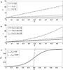 |
Fig. 1 Typical background density, temperature, and shear flow profiles. a) Temperature profiles for the different θ that were used. b) Density profiles for θ = 2 but three different polytropic indices m. For all indices m, the atmosphere is stably stratified. c) Shear flow profiles with the smallest and largest characteristic length Lu used are shown. |
2.2. Formulation of the Eigenvalue problem
In a diffusive model there are a number of different time scales, including the time scale associated with the shear dynamics tS = Lu/ (U0), the time scale for buoyancy tB = 1 /N(z), where N(z)2 is the Brunt-Väisälä frequency, and the time scale for thermal diffusion  . In this paper, we focus on the regime where the viscous time scale,
  , is much greater than any other time scales. This allows us to neglect viscous heating, which corresponds to the first term on the right-hand side in Eq. (3). In addition, the shear flow given by Eq. (9) is in equilibrium only if tμ is much greater than the instability time scale, which we verify a posteriori. When tμ becomes comparable to other relevant time scales, the background shear flow is not in equilibrium, and our analysis would be inappropriate for this case.
We perturb each quantity that appears in Eqs. (1)−(3) such that f = f0 + δf and  (10)where k ∈R and l ∈R are the horizontal wave numbers, and ζ = ζr + iζi ∈C, where ζr gives the growth rate of the linear instability.
We would like to stress that the equations for the perturbed quantities that we obtain do not inherit the same symmetry properties as the well known Taylor-Goldstein equation (e.g., Miles 1961), where taking the complex conjugate of the eigenfunction and eigenvalue leads to the same equation. This symmetry is broken in our set of equations, because there are still terms that are linear in k and l. Therefore, for our eigenvalue problem, there are not necessarily two complex conjugated solutions where one is decaying and one is a growing solution.
For our initial set of equations a Squire transformation exists to transform the three-dimensional problem to a corresponding two-dimensional one. The transformation can be written as
 (11)Having also checked numerically that indeed for a certain wave number k, the growth rate ζr decreases with increasing l, we can set l = 0 without loss of generality for our following computations. Denoting δu = (u,v,w), we obtain this linearised coupled set of equations
 where a similar set of equations was derived for a problem including magnetic fields by Tobias & Hughes (2004). Our system is characterised by six parameters m, θ, σ, Ck, U0, and Lu. Equations (13)−(15) are numerically solved on a one-dimensional grid in the z-direction that is discretised uniformly, and this method is adapted from the method used by Favier et al. (2012). Recasting the set of differential equations into the form
  (16)where the matrix A contains the finite difference coefficients applied to the discretised eigenfunctions f = (δρ,u,v,w,δT)T, reduces the problem to a matrix equation. To find the eigenvalues and vectors we use the Schur factorisation (Anderson et al. 1999). For computing the relevant coefficients in A, a central fourth-order finite differences scheme was used. We searched for the eigenvector solutions with the greatest real part of the eigenvalue ζ where the vertical velocity eigenvector, w, vanishes at the boundaries. Ultimately, we aim to do non-linear simulations with a pseudo-spectral code, at which point viscosity is mandatory. Therefore, most of the computations consider a viscous fluid.
3. Results
In this section we focus on a number of key areas. First, we present the change in the stability threshold while the Mach number is varied. The effect of compressibility is separately investigated in a weakly thermally stratified and a strongly thermally stratified atmosphere in Sect. 3.1. Later in Sect. 3.2, the growth rates of the linear shear instability, together with the critical Ri for different Péclet numbers, are compared, and the effect on the stability against buoyancy is discussed. In Sect. 3.2.1, the effect of different polytropic indices on the instability is addressed, and the possibility of a Holmboe like instability is investigated in Sect. 3.3.
3.1. The effect of varying the Mach number on the instability threshold
Because the Richardson criterion is based on simple energetic arguments and does not take compressibility into account, clarification is needed to determine whether compressibility affects the stability of a shear flow. Therefore, in this section we focus on the stability threshold for different Mach numbers in a viscous (we consider σ = 1.0 and Ck = 10-6) and stably stratified fluid with m = 1.6. Although stellar interiors typically have low Mach numbers, especially at the base of the convection zone, generally moderate-to-high Mach numbers can appear at the surface and in other astrophysical objects. Investigating the consequences of moderate Mach numbers on a shear flow is thus of general interest. In the following we refer to the Mach number, M(z), as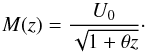 (17)This is the consequence of our previous definition, where velocity is given in units of the sound speed that is computed at the top of our domain. Because the inflexion point of our shear flow is at z = 0.5, and the sound speed varies with temperature, it is necessary to compute the actual Mach number, M, at z = 0.5.
According to Schochet (1994) and Guillard & Murrone (2004), the solutions of the compressible Euler equations reduce to the solutions of the incompressible Euler equations in the low Mach number limit. Thus, varying the Mach number allows the validity of the Richardson criterion to be investigated for low-to-moderate Mach numbers (0.02 <M< 0.15).
We make use of the general definition of the Brunt-Väisälä frequency given by 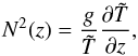 (18)where
  is the potential temperature, to define the local Richardson number as
 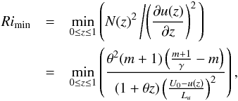 (19)where the derivative of the background velocity profile with respect to z corresponds to a local turnover rate of the shear.
To find the critical Richardson number, Ric, we solve the eigenvalue problem for a small Ri, while varying the wave number, k, between 0 and 1 /Lu to find the most unstable mode kmax. For a large, but finite, Reynolds number, the system is assumed to be stable if the growth rate, ζr, is zero for all wave numbers or the time scale for the instability, tζ = 1 /ζr, compared to the viscous time scale, tμ, is of the same order of magnitude.
A detailed survey for θ = 2, a weakly stratified atmosphere, and for θ = 10, a strongly stratified atmosphere, reveals that the critical Richardson number decreases for Mach numbers greater than 0.08, which can be seen in Fig. 2. For the majority of incompressible and weakly compressible Mach numbers, the critical Richardson number does not significantly deviate from the well known 1/4 threshold for stability. In the case of a weakly stratified atmosphere, the critical Richardson number decreases rapidly below 0.1 for M ≈ 0.14. In a strongly stratified fluid, we find the same behaviour as for the weakly stratified case qualitatively, but the critical Richardson number does not drop below 0.2 for M ≈ 0.14. The shift in the stability threshold in both a strong and a weakly stratified fluid and towards smaller Richardson numbers for moderate Mach numbers indicates a stabilising effect of compressibility on the KH instability. Though not focusing on KH-like instabilities alone, previous investigations of compressible shear flows with uniform temperature and without gravity for high Mach numbers revealed similar results; for example, Blumen et al. (1975) and Drazin & Davey (1977) have shown that for  , the system becomes stable. In this system two types of unstable modes are present for Mach numbers greater than 0.94, which are stationary modes and travelling modes.
In the case of KH-like instabilities, one explanation for the stabilising effect for Mach numbers greater than 0.08 is as follows. For an incompressible fluid, the classical Richardson criterion uses simple energetic arguments, where two neighbouring fluid parcels are exchanged. The density of these parcels remains constant such that only the change in velocity (at different heights) changes the kinetic energy, ΔEkin, and changes in the potential energy, ΔEpot, are solely due to the changes in position of the fluid parcel. While for a compressible fluid the density will decrease to a certain amount when a fluid parcel is moved up adiabatically, such that a part of the kinetic energy is converted by the process of expansion, more kinetic energy is needed to reach the instability threshold, which requires a greater velocity gradient.
 |
Fig. 2 Critical Richardson number in a viscous fluid for different Mach numbers, M, in both plots. The corresponding wave numbers kmax of the most unstable mode at the onset of instability are plotted, and the wave number is normalised by the inverse of the characteristic length 1 /Lu. The horizontal line in both plots corresponds to Ri = 0.25. In a) the atmosphere is weakly stratified with θ = 2, whereas in b)θ = 10, which corresponds to a strongly stratified atmosphere. |
Different temperature gradients have a non-trivial effect on the effective Mach number throughout our domain, where M changes according to Eq. (17). In the limit of weak thermal stratification, M remains almost constant, whereas in a strongly stratified atmosphere it changes significantly and generates an asymmetry between the regions above and below the shear flow. The observed asymmetry changes the eigenfunctions found for a fixed M(z = 0.5) and Lu, which are shown in Fig. 3. Because M(z = 0.5) and Lu are fixed, increasing θ is equivalent to increasing the Richardson number (see Eq. (19)). The asymmetry with respect to the mid-plane is clearly visible in the temperature and vertical velocity eigenfunctions for the strongly stratified case θ = 10 (see Figs. 3a and b), whereas the same eigenfunctions are much more symmetric for θ = 2 (see Figs. 3d and e). This asymmetry has an impact on the observed deviation between the change in the critical Richardson number for θ = 2 and θ = 10. In fact, in a stratified atmosphere, exchanged fluid parcels, where the one that is shifted downwards from the middle plane z = 0.5 and the other upwards, move at the same speed in opposite directions, but have different Mach numbers. With an increasing temperature gradient, the effective Mach number in the lower half of our domain has a steeper drop such that the stabilising effect of compressibility vanishes. Therefore, the stabilising effect of greater Mach numbers in a strongly stratified atmosphere is weaker.
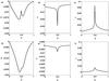 |
Fig. 3 Eigenfunctions for a fixed M = 0.114 and a fixed characteristic length scale Lu = 0.09 for two different θ, where θ = 2 for the plots d), e), f), and θ = 10 for upper plots a), b), c). In both cases the eigenfunctions for the most unstable mode are shown. |
3.2. Small Péclet number regime
In the following we focus on the impact of thermal diffusion in a stably stratified fluid. For non-negligible thermal diffusion, the non-dimensional Péclet number is given as  (20)where Lu is the characteristic length of the shear width and U0 corresponds to the Mach number at the top of the domain because the velocity is normalised with respect to the sound speed. The Péclet number is associated with the ratio of advective transport to thermal diffusion.
Varying the Péclet number in an inviscid compressible fluid enhances the results found by Lignières et al. (1999) where a higher thermal diffusion destabilises the system because it effectively weakens the stable stratification; i.e., the system becomes less stable against buoyancy. Therefore, thermal diffusion becomes important in a system where tk<tB, such that buoyancy is much slower than thermal diffusion. Since tB has to be smaller than the system’s dynamic time scale tS, the Péclet number has to become smaller than unity to satisfy these requirements.
In Fig. 4 the growth rates for different Péclet numbers in a compressible and a weakly compressible fluid are illustrated. Comparing instability growth rates for a set up with Pe< 1 and Pe> 1 shows that ζr increases with decreasing Pe, where a significant jump can be observed when Pe becomes smaller than unity. We find that the overall growth rate is smaller for a shear flow with Mach number equal to 0.09, this demonstrates the stabilising effect of moderate Mach numbers as discussed in Sect. 3.1. However, an increase in the instability growth rate does not necessarily indicate a shift in the stability threshold to greater Richardson numbers.
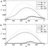 |
Fig. 4 Growth rates ζr in an inviscid, weakly thermally stratified atmosphere with θ = 0.5 for a Richardson number of Ri = 0.22. In a) the fluid is compressible with M = 0.09 and in b) M = 0.009, which corresponds to a incompressible fluid. The Péclet number is varied among three orders of magnitude. |
When focusing on the stability threshold, it is necessary to seek the critical Richardson numbers in different Péclet number regimes. For previous calculations of the growth rates, the fluid was assumed to be inviscid to simplify the problem and to avoid the problem of the initial state not actually being an equilibrium state. Here, it is more convenient to include viscosity because it is numerically easier to obtain results for the limit of low viscosity than for an inviscid fluid.
For a shear flow the onset of instability does not change for small enough k, if large enough Reynolds numbers are considered. However, including viscosity may have non-trivial effects on the stability if the fluid has high thermal diffusivity (see Jones 1977). Jones (1977) derived a criterion for instability at long wavelengths in the form kPeRi< 0.086 in an inviscid fluid. For a viscous fluid it can be rewritten as kσReRi< 0.086 such that for reasonably small wave numbers, the system can still be unstable if the Reynolds number is not sufficiently large. It can be partly seen when investigating Eqs. (14) and (15), where almost all terms include the wave number, while one of the three viscous terms does not. Therefore, for small wave numbers, this viscous term, which is proportional to the second derivative in z direction, becomes relatively more important for the dynamics of the system. To make certain that the results correspond to a regime where viscosity does not affect the stability threshold, several computations were repeated with less viscosity and with a greater viscosity than used in the actual computations.
In Fig. 5 curves of marginal stability for four different Péclet numbers in a polytropic atmosphere are displayed for θ = 0.5 and θ = 2.0. As expected, the domain for an unstable shear flow increases as the Péclet number is decreased. It shows that not only is the growth rate of the instability altered but the stability threshold also changes for small Péclet numbers. The critical Richardson numbers for Pe ≤ 1 reveal a destabilisation for small k. Lignières et al. (1999) explained this behaviour by the effect of the anisotropy of the buoyancy force. The stabilising effect of stratification becomes inefficient for predominant horizontal motion compared to the thermal diffusion. Indeed, by computing the ratio of the vertical-to-horizontal kinetic energy of the unstable mode for a certain k, i.e.  (21)where wk(z) and uk(z) are the eigenfunctions for the vertical and horizontal velocity disturbances at a certain k respectively, we are able to investigate the nature of the instability. Comparing this ratio for a mode with k = 0.1 and k = 0.7 for Pe = 0.1, it turns out that the ratio for the larger k-mode is two orders of magnitude greater than for the smaller k-mode. Thus the horizontal motion associated with larger wave lengths in the horizontal direction is predominant at very small k.
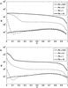 |
Fig. 5 Critical Richardson numbers for all k in a viscous fluid with a Mach number, M = 0.009, a)θ = 0.5 and b)θ = 2.0 and viscosity (σCk) of order 10-7. The Péclet number is varied from 10 to 0.01. |
The results carried out for a greater temperature gradient, θ = 2 shown in Fig. 5b, reveal a qualitatively different behaviour for the small Péclet numbers than is the case for θ = 0.5 shown in Fig. 5a. The θ = 0.5 case has an overall greater critical Richardson number, but there is a gradual increase towards a smaller critical Richardson number in the small k limit. This indicates a more efficient destabilisation for most of the wave numbers and a less efficient destabilisation for small k.
Looking again at the ratio of kinetic energy in vertical and horizontal motions reveals that for lower θ the ratio of vertical motions to horizontal motions remains significantly smaller than for the higher stratification θ = 2, which indicates that buoyancy force is more efficient in a strongly stratified atmosphere against the destabilising effect of thermal diffusion. A weakly stratified atmosphere can be destabilised quicker by thermal diffusion.
3.2.1. Effect of the distance to the onset of convection on the instability
The destabilising mechanism of thermal diffusion can be traced back to the fact that thermal diffusion weakens the stable stratification against buoyancy. To investigate whether and how this effect changes if the system is farther away from the onset of convection, the polytropic index is varied between 1.6, which is close to the threshold, and 2.07, which is far from the onset of convection. In Fig. 6a the growth rate, ζr, is plotted for different polytropic indices, while the Richardson number is fixed to the value Ri = 0.22 and the Péclet number is unity. The growth rate is given in units of the sound speed, such that a rescaling is necessary, while the amplitude of the shear flow is adjusted to keep Ri constant. The same is done for a Péclet number of 0.1 in Fig. 6b where the same tendency of an increasing growth rate with increasing polytropic index is observed. To exclude that this behaviour is the effect of thermal diffusion, the growth rate for two different m is computed for a fixed Ri smaller than 1/4 for much greater Pe than unity, where the same tendency is found. However, the critical Ri increases as m is varied upwards. Therefore, a system with greater polytropic index, m, is less stable such that for the same Ri, the system with a greater m is farther away from the stability threshold and has a higher growth rate. Non-linear direct numerical computations of two cases approved the results obtained with the linear EV solver. For this purpose Eqs. (1)−(3) were solved by using a hybrid finite-difference/pseudo-spectral code (see for example Matthews et al. 1995; Silvers et al. 2009a,b, and references therein).
While increasing the polytropic index requires a greater shear flow amplitude to obtain the same ratio between the buoyancy force and the turnover rate, the available kinetic energy of the system is increased. Consequently, as soon as the system can overcome the stabilising effect of density stratification, the instability has more available kinetic energy from which it can grow more rapidly.
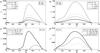 |
Fig. 6 Growth rates for the linear instability in an inviscid fluid with thermal stratification θ = 2.0 and low Mach number of the order of 10-2. In a) and c) the Péclet number is equal to unity and in b) and d) Pe = 0.1. Ri is varied at the two bottom plots c) and d) but it is fixed to Ri = 0.22 for the top plots a) and b). |
In the two plots at the bottom of Fig. 6, the growth rates for different polytropic indices are shown while all other parameter are held. The solid lines in Figs. 6c and d correspond to the solid lines in Figs. 6a and b, respectively. As expected, the instability growth rate decreases with increasing density stratification and greater Ri. While for a Péclet number of unity the instability shuts down rapidly, which is displayed in Fig. 6c, for Pe< 1 the same behaviour is observed, but the instability for greater m is still present for small wave numbers. As discussed in Sect. 3.2, this is explained by the anisotropy of the buoyancy force.
3.3. Subdominant shear instability
For certain configurations where the shear width is small enough, the velocity profile is similar to two counter flows. Then, for a stable stratification and Péclet numbers much greater than unity, a Holmboe-like instability is found. The Holmboe instability, which was introduced by Holmboe (1962), results from interacting waves that propagate in opposite directions (Baines & Mitsudera 1994). The Holmboe instability differs from the KH instability in several ways (see the review article by Peltier & Caulfield 2003). First, the KH instability is stationary in a frame of reference, but the Holmboe instability has counter-propagating unstable modes, which both have the same growth rate. One mode occupies the upper plane and the other the lower plane, such that a superposition of both solutions form a standing-wave solution. Second, the Holmboe instability is favoured in stable stratified atmospheres and can dominate the Kelvin-Helmholtz instability when the stratification stability is increased, such that a KH instability disappears because of the Richardson criterion (Peltier & Smyth 1989).
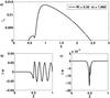 |
Fig. 7 Growth rate for an inviscid fluid with a temperature gradient, θ = 1.0, Péclet number of the order of 103 and Ri = 0.3 in plot a). The form of the eigenfunctions found for the vertical velocity w in the small arch and the large arch are displayed in b) and c), respectively. |
In Fig. 7a two arches are present. The one with the greater maximum growth rate appears at greater k and corresponds to the KH instability, whereas only one unstable mode is present for a certain wave number, and its phase velocity corresponds to the mean flow velocity. The eigenfunction for the vertical velocity of these modes is shown in Fig. 7c, which reveals that the instability is localised at the centre of the shear flow. Unstable modes with k corresponding to the smaller arch exhibit all properties of the Holmboe instability, where two counter-propagating modes are present, one in the upper and one in the lower half plane. Figure 7b shows the form of the vertical velocity eigenfunction that is propagating in the lower half plane, and the corresponding mode with the opposite phase velocity shows the oscillations in the upper half plane. Investigating all possible eigenfunctions at the overlap region between the two arches reveals that Holmboe modes are present but have a lower growth rate as the KH instability or vice versa.
The observed Holmboe-like instability only appears for large Péclet numbers, while for small Pe, the range for the KH instability is enlarged to smaller wave numbers, such that even in the presence of the Holmboe-like instability, the KH instability for the same wave numbers dominates. This can be seen in Figs. 6a and b, where a small shoulder is present in the range 0.35 <k< 0.5 in a) for Pe = 1 and is dominated by the KH instability in b) for Pe = 0.1.
To make certain that these modes are physical and not a numerical artefact, we checked that they remain for a system where we assume an inviscid non-diffusive incompressible fluid. In a second check, we considered a non-uniform grid distribution in the z direction, with more resolution where the largest gradients are observed. With both approaches a second instability, with the same properties, was found at slightly smaller wave numbers, k, than the KH instability. Using non-linear computations, both instabilities are found during the linear growth regime with similar growth rates and eigenfunctions, as predicted from the linear computations.
4. Conclusions
Shear flow instabilities, which may lead to turbulent motions, are important for understanding the dynamics in stellar interiors and in other astrophysical flows. Using linear stability analysis, the onset of shear flow instability in a compressible polytropic atmosphere was investigated, where a detailed analysis of the effect of moderate Mach numbers, small Péclet numbers and different polytropic indices was carried out separately.
For a flow of moderate Mach numbers, we found a stabilising effect that results in a critical Richardson number that is less than 1/4, such that for a certain range of Ri less than 1/4, the shear flow remains stable to KH instability. This effect becomes significant for Mach numbers greater than 0.1. However, the stabilising is weaker for strongly stratified atmospheres. Because this effect is most relevant at moderate-to-high Mach numbers, it can be neglected for most stellar regions, in particular for the tachocline. However, this result might be important in other astrophysical objects where high Mach numbers are common.
For fluids with high thermal diffusivity, where the Péclet number drops below unity, a destabilisation of the system can be shown. Our results agree with Lignières et al. (1999), where the regime of small Péclet numbers were examined in a Boussinesq fluid. We find a significantly greater growth rate for highly diffusive fluids and greater critical Richardson numbers for Pe< 1 than in systems with large Péclet numbers. Generally, steeper temperature gradients lead to an overall stabilisation for small Péclet numbers. However, it should be noted that, for very small wave numbers, we found that the opposite is true because of the anisotropy of the buoyancy force.
An interesting result is that we find the possibility of Holmboe-like instabilities present in polytropic atmopheres. This instability is dominated by the KH instability for small Péclet numbers, but is clearly present for large Péclet numbers. While no setup was found where the Holmboe-like instability dominates the KH instability, it may be found in future investigations.
Studying more complex systems, which include key properties of stars, by means of a linear stability analysis provides a powerful tool for investigating their linear behaviour. However, the vertical length scale for which these shear flows can become
unstable is far below the resolution of helioseismological techniques, and since the perturbation’s amplitude can be finite in the tachocline (see Michaud & Zahn 1998), the assumption of infinitesimal perturbations made in the stability analysis might lead to different results. To deal with that issue, it is necessary to investigate the stability properties of such flows by means of direct numerical computations, where the initial state is perturbed by perturbations with a finite amplitude. In addition to finite amplitude effects, the non-linear behaviour of unstable shear flows after a saturation is crucial for understanding the mixing in stellar interiors regardless of the nature of the initial instability.
Having established an understanding of the hydrodynamical problem, further non-linear investigations are underway to obtain a full picture.
Acknowledgments
This research has received funding from STFC and from the School of Mathematics, Computer Science and Engineering at City University London. We would also like to thank the anonymous referee for helpful comments.
References
- Anderson, E., Bai, Z., Bischof, C., et al. 1999, LAPACK Users’ Guide: Third Edition, Software, Environments, and Tools (Philadelphia: Society for Industrial and Applied Mathematics) [Google Scholar]
- Baines, P. G., & Mitsudera, H. 1994, J. Fluid Mech., 276, 327 [NASA ADS] [CrossRef] [Google Scholar]
- Blumen, W., Drazin, P. G., & Billings, D. F. 1975, J. Fluid Mech., 71, 305 [NASA ADS] [CrossRef] [Google Scholar]
- Charney, J. G. 1947, J. Meteor, 4, 135 [CrossRef] [Google Scholar]
- Christensen-Dalsgaard, J., & Thompson, M. J. 2007, in The Solar Tachocline, eds. D. W. Hughes, R. Rosner, & N. O. Weiss (Cambridge University Press), 53 [Google Scholar]
- Drazin, P. G., & Davey, A. 1977, J. Fluid Mech., 82, 255 [Google Scholar]
- Drazin, P. G., & Reid, W. H. 2004, Hydrodynamic Stability, 2nd edn. (Cambridge University Press) [Google Scholar]
- Dudis, J. J. 1974, J. Fluid Mech., 64, 65 [NASA ADS] [CrossRef] [Google Scholar]
- Favier, B., Jouve, L., Edmunds, W., Silvers, L. J., & Proctor, M. R. E. 2012, MNRAS, 426, 3349 [NASA ADS] [CrossRef] [Google Scholar]
- Guillard, H., & Murrone, A. 2004, Computers & Fluids, 33, 655 [Google Scholar]
- Holmboe, J. 1962, Geophys. Publ., 24, 67 [Google Scholar]
- Jones, C. A. 1977, Geophy. Astro. Fluid Dyn., 8, 165 [NASA ADS] [CrossRef] [Google Scholar]
- Kosovichev, A., Schou, J., Scherrer, P., et al. 1997, Sol. Phys., 170, 43 [NASA ADS] [CrossRef] [Google Scholar]
- Lignières, F., Califano, F., & Mangeney, A. 1999, A&A, 349, 1027 [NASA ADS] [Google Scholar]
- Matthews, P. C., Proctor, M. R. E., & Weiss, N. O. 1995, J. Fluid Mech., 305, 281 [NASA ADS] [CrossRef] [Google Scholar]
- Michaud, G., & Zahn, J.-P. 1998, Theor. Comp. Fluid Dyn., 11, 183 [Google Scholar]
- Miczek, F. 2013, Ph.D. Thesis, Technical University of Munich [Google Scholar]
- Miesch, M. S. 2007, in The Solar Tachocline, eds. D. W. Hughes, R. Rosner, & N. O. Weiss (Cambridge University Press), 109 [Google Scholar]
- Miles, J. W. 1961, J. Fluid Mech., 10, 496 [NASA ADS] [CrossRef] [Google Scholar]
- Ofman, L., & Thompson, B. J. 2011, ApJ, 734, L11 [NASA ADS] [CrossRef] [Google Scholar]
- Peltier, W. R., & Caulfield, C. P. 2003, Ann. Rev. Fluid Mech., 35, 135 [NASA ADS] [CrossRef] [Google Scholar]
- Peltier, W. R., & Smyth, W. D. 1989, J. Atm. Sci., 46, 3698 [NASA ADS] [CrossRef] [Google Scholar]
- Schatzman, E., Zahn, J.-P., & Morel, P. 2000, A&A, 364, 876 [NASA ADS] [Google Scholar]
- Schochet, S. 1994, J. Differ. Equations, 114, 476 [Google Scholar]
- Silvers, L. J. 2008, Philos. T. Roy. Soc. A, 366, 4453 [NASA ADS] [CrossRef] [Google Scholar]
- Silvers, L. J., Bushby, P. J., & Proctor, M. R. E. 2009a, MNRAS, 400, 337 [NASA ADS] [CrossRef] [Google Scholar]
- Silvers, L. J., Vasil, G. M., Brummell, N. H., & Proctor, M. R. E. 2009b, ApJ, 702, L14 [NASA ADS] [CrossRef] [Google Scholar]
- Tobias, S. M. 2004, in Fluid Dynamics and Dynamos in Astrophysics and Geophysics, eds. A. M. Soward, C. A. Jones, D. W. Hughes, & N. O. Weiss (London: CRC), 193 [Google Scholar]
- Tobias, S. M., & Hughes, D. W. 2004, ApJ, 603, 785 [NASA ADS] [CrossRef] [Google Scholar]
- Zahn, J.-P. 1974, in Stellar Instability and Evolution, eds. P. Ledoux, A. Noels, A. Rodgers, (Dordrecht: Reidel), 185 [Google Scholar]
All Figures
|
Fig. 1 Typical background density, temperature, and shear flow profiles. a) Temperature profiles for the different θ that were used. b) Density profiles for θ = 2 but three different polytropic indices m. For all indices m, the atmosphere is stably stratified. c) Shear flow profiles with the smallest and largest characteristic length Lu used are shown. |
| In the text | |
|
Fig. 2 Critical Richardson number in a viscous fluid for different Mach numbers, M, in both plots. The corresponding wave numbers kmax of the most unstable mode at the onset of instability are plotted, and the wave number is normalised by the inverse of the characteristic length 1 /Lu. The horizontal line in both plots corresponds to Ri = 0.25. In a) the atmosphere is weakly stratified with θ = 2, whereas in b)θ = 10, which corresponds to a strongly stratified atmosphere. |
| In the text | |
|
Fig. 3 Eigenfunctions for a fixed M = 0.114 and a fixed characteristic length scale Lu = 0.09 for two different θ, where θ = 2 for the plots d), e), f), and θ = 10 for upper plots a), b), c). In both cases the eigenfunctions for the most unstable mode are shown. |
| In the text | |
|
Fig. 4 Growth rates ζr in an inviscid, weakly thermally stratified atmosphere with θ = 0.5 for a Richardson number of Ri = 0.22. In a) the fluid is compressible with M = 0.09 and in b) M = 0.009, which corresponds to a incompressible fluid. The Péclet number is varied among three orders of magnitude. |
| In the text | |
|
Fig. 5 Critical Richardson numbers for all k in a viscous fluid with a Mach number, M = 0.009, a)θ = 0.5 and b)θ = 2.0 and viscosity (σCk) of order 10-7. The Péclet number is varied from 10 to 0.01. |
| In the text | |
|
Fig. 6 Growth rates for the linear instability in an inviscid fluid with thermal stratification θ = 2.0 and low Mach number of the order of 10-2. In a) and c) the Péclet number is equal to unity and in b) and d) Pe = 0.1. Ri is varied at the two bottom plots c) and d) but it is fixed to Ri = 0.22 for the top plots a) and b). |
| In the text | |
|
Fig. 7 Growth rate for an inviscid fluid with a temperature gradient, θ = 1.0, Péclet number of the order of 103 and Ri = 0.3 in plot a). The form of the eigenfunctions found for the vertical velocity w in the small arch and the large arch are displayed in b) and c), respectively. |
| In the text | |
Current usage metrics show cumulative count of Article Views (full-text article views including HTML views, PDF and ePub downloads, according to the available data) and Abstracts Views on Vision4Press platform.
Data correspond to usage on the plateform after 2015. The current usage metrics is available 48-96 hours after online publication and is updated daily on week days.
Initial download of the metrics may take a while.