| Issue |
A&A
Volume 576, April 2015
|
|
|---|---|---|
| Article Number | L16 | |
| Number of page(s) | 4 | |
| Section | Letters | |
| DOI | https://doi.org/10.1051/0004-6361/201525969 | |
| Published online | 16 April 2015 | |
No asymmetric outflows from Sagittarius A* during the pericenter passage of the gas cloud G2
1 Department of Physics and Astronomy, Seoul National University, 1 Gwanak-ro, Gwanak-gu, 151-742 Seoul, Korea
e-mail: jhpark@astro.snu.ac.kr; trippe@astro.snu.ac.kr
2 Max-Planck-Institut für Radioastronomie (MPIfR), Auf dem Hügel 69, 53121 Bonn, Germany
3 Korea Astronomy and Space Science Institute (KASI), 776 Daedeokdae-ro, Yuseong-gu, 305-348 Daejeon, Korea
4 Institute of Geodesy and Geoinformation, Bonn University, Nussallee 17, 53115 Bonn, Germany
5 Institut de Radioastronomie Millimétrique (IRAM), 300 rue de la Piscine, 38406 Saint-Martin d’ Hères, France
6 Observatorio Astronomico Nacional (IGN), Observatorio de Yebes, Aptdo. 148, Yebes, 19080 Guadalajara, Spain
Received: 26 February 2015
Accepted: 31 March 2015
The gas cloud G2 that falls toward Sagittarius A* (Sgr A*), the supermassive black hole at the center of the Milky Way, is assumed to provide valuable information on the physics of accretion flows and the environment of the black hole. We observed Sgr A* with four European stations of the Global Millimeter Very Long Baseline Interferometry Array (GMVA) at 86 GHz on 1 October 2013 when parts of G2 had already passed the pericenter. We searched for a possible transient asymmetric structure – such as jets or winds from hot accretion flows – around Sgr A* that might be caused by accretion of material from G2. The interferometric closure phases remained zero within errors during the observation time. We therefore conclude that Sgr A* did not show significant asymmetric (in the observer frame) outflows in late 2013. Using simulations, we constrain the size of the outflows that we could have missed to ≈2.5 mas along the major axis and ≈0.4 mas along the minor axis of the beam, corresponding to approximately 232 and 35 Schwarzschild radii, respectively; we thus probe spatial scales on which the jets of radio galaxies are thought to convert magnetic into kinetic energy. Because probably less than 0.2 Jy of the flux from Sgr A* can be attributed to accretion from G2, the effective accretion rate is ηṀ ≲ 1.5 × 10⁹ kg s-1 ≈ 7.7 × 10⁻⁹M⊕ yr-1 for material from G2. Exploiting the relation of kinetic jet power to accretion power of radio galaxies shows that the rate of accretion of matter that is finally deposited in jets is limited to Ṁ ≲ 1017 kg s-1 ≈ 0.5 M⊕ yr-1. Accordingly, G2 appears to be mostly stable against loss of angular momentum and subsequent (partial) accretion at least on timescales ≲1 yr.
Key words: accretion, accretion disks / black hole physics / Galaxy: center / radio continuum: general
© ESO, 2015
1. Introduction
With a mass of M• ≈ 4.3 × 10⁶M⊙ and located at the center of the Milky Way at a distance of R0 ≈ 8 kpc, Sagittarius A* (Sgr A*) is the nearest supermassive black hole (see, e.g., Genzel et al. 2010 for a review). Thanks to its proximity, the Galactic center serves as an excellent laboratory for the astrophysics of galactic nuclei; for the given mass and distance, 1 m ≡ 8 a.u. ≡ 94 RS, with RS denoting the Schwarzschild radius. Sgr A* is characterized by its low luminosity compared to active galactic nuclei (AGN), with a bolometric luminosity ≲2 × 10⁻⁸ of its Eddington luminosity (see Narayan et al. 1998 and references therein). Sgr A* shows a slightly inverted radio spectrum peaking at mm-to-submm wavelengths (Zylka et al. 1992; Falcke et al. 1998; Melia & Falcke 2001; Bower et al. 2015).
The emission mechanism of Sgr A* is a matter of ongoing debate. On the one hand, radiatively inefficient accretion flows (RIAFs; e.g., Yuan et al. 2003) successfully reproduce the observed fluxes at various wavelengths. On the other hand, multiple studies (Falcke & Markoff 2000; Markoff et al. 2001, 2007; Yuan et al. 2002; Falcke et al. 2009) have pointed out that parts of the emission need to originate from jets, which is supported by observational evidence for the presence of jets (Yusef-Zadeh et al. 2012; Li et al. 2013). The current lack of structural information on Sgr A* prevents an unambiguous decision between competing theories. At the short-wavelength side of the submm-bump, where the emission becomes optically thin, instruments with the necessary spatial resolution are not available. At wavelengths of more than a few millimeters, the source structure is washed out by interstellar scattering (e.g., Bower et al. 2006). Lu et al. (2011) found evidence that the shape and orientation of the elliptical Gaussian changes with frequency; this could be interpreted as an intrinsic structure that is slightly misaligned with the scattering disk, which shines through toward higher frequencies. In addition, recent Very Long Baseline Interferometry (VLBI) observations at 43 GHz have been able to resolve an intrinsic elliptical structure with a preferred geometrical axis (Bower et al. 2014). This structure might indicate an existence of jets, but could also be the result of an elongated accretion flow such as a black hole crescent (e.g., Kamruddin, & Dexter 2013).
Recently, a gas cloud labeled G2 was observed to move toward Sgr A* on a nearly radial orbit (Gillessen et al. 2012). So far, mainly two possible structures of G2 have been discussed, with the first scenario being that G2 is a localized overdense region within an extended gas streamer. This agrees with observations reporting that G2 is composed of a compact head and a more widespread tail (Gillessen et al. 2013b; Pfuhl et al. 2015). The two components are on approximately the same orbit and are connected by a faint bridge in position-velocity diagrams, in Gillessen et al. (2013a) and lasted over one year,while G2 has been stretched substantially along its orbit by tidal shearing caused by the gravitational potential of Sgr A* (Pfuhl et al. 2015). Test particle simulations have provided a good explanation for the dynamics of G2; the results showed that hydrodynamic effects have not been significant (e.g., Pfuhl et al. 2015; see also Schartmann et al. 2012). The second possibility under discussion is that G2 is a circumstellar cloud around a star that provides stabilizing gravity and continuously replenishes the gas. Studies supporting this scenario highlighted that the tail might only be a fore- or background feature and might not be physically connected to G2 (Phifer et al. 2013; Valencia et al. 2015). Recent observations have also shown that G2 survived its pericenter passage as a compact source, which might be a clue that G2 is a star enshrouded by gas and/or dust (Witzel et al. 2014; Valencia et al. 2015). This scenario was modeled analytically (Miralda-Escudé 2012; Scoville & Burkert 2013) and explored with the help of numerical simulations (Ballone et al. 2013; De Colle et al. 2014; Zajaček et al. 2014).
Interactions with the accretion flows toward Sgr A* might cause G2 to lose angular momentum, and as a result, parts of it may be accreted by the black hole (Anninos et al. 2012; Burkert et al. 2012; Schartmann et al. 2012). Accordingly, an increased radio luminosity (e.g., Mahadevan 1997; Mościbrodzka et al. 2012) as well as an increase in source size might be expected (e.g., Mościbrodzka et al. 2012). In addition, radio-bright outflows such as jets or wind-like outflows related to RIAFs (Yuan et al. 2003; Mościbrodzka et al. 2012; Liu & Wu 2013) might become observable on spatial scales of ≲1 mas. To search for such transient structures, we performed VLBI observations with four European stations of the Global Millimeter VLBI Array (GMVA) at 86 GHz, providing an angular resolution down to ≈0.3 mas. Our observing frequency of 86 GHz is in a region where scattering vanishes and is weaker in the images of Sgr A* at frequencies lower than about 43 GHz (Bower et al. 2004, 2006; Shen et al. 2005).
2. Observations and data analysis
We observed Sgr A* at 86 GHz on 1 October 2013 using four GMVA stations of the European VLBI Network (EVN): Effelsberg (EF), Pico Veleta (PV), Plateau de Bure (PB), and Yebes (YS). A combination of the low declination of Sgr A* (−29°), the high latitude of the stations (the minimum latitude being 37° for Pico Veleta), and a technical problem at Yebes station limited our observing times to around 1.5 h for Yebes and 2.5 h for the other stations. We observed both circular polarizations except for Yebes station, where only left circular polarization (LCP) data were obtained. The data were recorded with the Mark 5 VLBI system (two-bit sampling) using the digital baseband converter (DBBC) in polyphase-filter bank mode with a bandwidth of 32 channels, each 16 MHz wide (total bandwidth 512 MHz). All data were correlated with the DifX VLBI correlator of the MPIfR (Bonn, Germany). Our calibrators (fringe-finding sources) were NRAO 530 and 1633+38.
We followed the standard procedures for initial phase and amplitude calibration using the AIPS software package (Greisen 2003) and applied phase self-calibration using the Caltech Difmap package (Shepherd 1997) with a point-source model. The geometry of our observation resulted in a very elongated beam (point spread function) with full widths at half maximum (FWHM) of 3.02 mas and 0.33 mas, respectively, at a position angle of −22°. For the flux density of Sgr A* we found a value of ≈1.4 ± 0.3 Jy).
We used the evolution of closure phases to search for asymmetric, extended emission around Sgr A*. A closure phase is the sum of the interferometric phases of the three baselines in a closed triangle of stations; it is free from antenna-based phase errors (e.g., Thompson et al. 2001). The closure phase for a centrally symmetric brightness distribution is zero. The amount of deviation from zero and the timescales of fluctuations of the closure phases can be used to probe the structure of an asymmetric source even if it cannot be imaged (due to lack of flux or insufficient uv plane coverage). This technique was previously used by Krichbaum et al. (2006) and Lu et al. (2011), who found the closure phases of Sgr A* to be consistent with zero throughout their observations in October 2005 and May 2007.
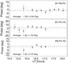 |
Fig. 1 Closure phases vs. time for three independent VLBI triangles. Each data point denotes a closure phase measurement averaged over one scan of six minutes; error bars correspond to 1σ errors. Dotted lines indicate weighted averages of all data points, dashed lines represent the corresponding standard errors of mean. Average phase values are noted in each diagram. Phases for the triangle EF-PB-PV are extracted from Stokes I data, phases for the other triangles from LL data. |
We extracted the closure phases from the visibility data for three independent triangles of the VLBI stations, initially binned into 10-second time bins. We flagged data with large errors (larger than the standard deviation of the data for a given triangle) and obvious outliers. The fraction of flagged data is 8.9%, 7.9%, and 6.0% for the triangles EF-PB-PV, EF-PV-YS, and PB-PV-YS, respectively; the difference between the results obtained with and without flagging is insignificant, however. We took the weighted average of the remaining values for each scan of 6 min; the resulting data set is shown in Fig. 1. We obtained a combined reduced χ2 value of 1.34 for all the closure phases for all the independent triangles based on the null hypothesis that the closure phase is zero all the time. The corresponding false-alarm probability (p-value) is 0.136; this value is clearly too high to reject the null hypothesis (this outcome did not change when choosing bin sizes other than 6 min). Consequently, we conclude that the closure phases agree with zero during the observing time.
3. Discussion
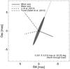 |
Fig. 2 Outflow orientations assumed in our simulation. The gray ellipse (with FWHM and position angle as noted) indicates the beam, dashed lines indicate four outflow orientations: along the major axis, along the minor axis, along the jet direction claimed by Li et al. (2013), and along the direction claimed by Yusef-Zadeh et al. (2012). |
The absence of a deviation of the closure phases from zero – within typical errors of a few degrees – implies the absence of asymmetric structure around Sgr A* at the time of our observation. A priori, bipolar, symmetric jets can account for zero closure phases. However, if the jet axis is oriented partly along the line of sight, the flux observed from the jet approaching the observer (f+) is amplified while that from the receding jet (f−) is dimmed by the Doppler effect. If the jets on both sides of the black hole have the same luminosity intrinsically, the observed ratio of the two fluxes is 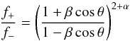 (1)(e.g., Beckmann & Shrader 2012), where β is the jet speed in units of speed of light, θ is the angle between the jet axis and the line of sight, and α is the spectral index defined via the flux density Sν ∝ να. Various observational constraints (α ≈ 0.5, β ≲ 0.1; Lu et al. 2011) and model predictions for transient jets (θ ≈ 60°, β ≈ 0.7; Falcke et al. 1998, 2009) place the flux ratios to be expected at between ≈1 and ≈6. Accordingly, even intrinsically symmetric jets from Sgr A* might appear asymmetric in the observer frame.
To constrain the size of outflows that we could have missed, we performed simple simulations. We placed artificial, unipolar secondary sources next to a primary point source model representing Sgr A* and compared the closure phases obtained from the resulting artificial visibility data with the observations. We considered two geometries: a single-point source and a jet composed of ten equally spaced point sources (knots) with equal fluxes. We probed four orientations for the simulated outflows (see Fig. 2): along the major axis, along the minor axis of the beam, the jet direction claimed by Li et al. (2013), and the jet direction claimed by Yusef-Zadeh et al. (2012). We used total fluxes of 0.2 Jy and 0.55 Jy for the artificial sources; these values ensure that our simulated outflows are sufficiently faint to not violate the constraints given by the known recent brightness evolution of Sgr A* (0.2 Jy from the mean variability of ≈15% from June 2013 to February 2014 at 41 GHz, with 0.55 Jy corresponding to the strongest variation in the same period, Chandler & Sjouwerman 2014). For each simulation setup, we measured the average of absolute values of the closure phases for each triangle. We varied the distances of the model sources (for the jet model: the largest distance) from Sgr A* until we found a critical distance at which the absolute values of the simulated closure phases exceeded those of the observations by more than the 1σ error at all triangles. We summarize our results in Table 1. As expected, the critical distances are smaller for brighter outflows. Jet-like structures lead to larger critical distances than equally luminous single, compact sources. As a consequence of the very elongated beam, the critical distances for sources located along the major axis of the beam are larger by a factor of ≈7 than for those located along the minor axis. In a few cases (denoted “N/A” in Table 1), the absolute values of the simulated closure phases were similar to those of the observations for all distances of the model sources, meaning that we were unable to identify a critical distance. Overall, our observations limit the extension of asymmetric (in the observer frame) jet-like outflows from Sgr A* to projected distances of ≈2.5 mas along the major axis and ≈0.4 mas along the minor axis.
Size constraints for outflows from Sgr A*.
Our analysis limits the (projected) extension of linear outflows to about 232 and 35 Schwarzschild radii, respectively, for outflows with fluxes of about 0.2 Jy; obviously, outflows substantially fainter could be larger and still remain undetected. Unfortunately, the resolution of our observations is not sufficient to probe structures in accretion flows that are expected to occur on scales ≲10 RS (cf., e.g., Broderick et al. 2011); those observations will probably have to await the Event Horizon Telescope (cf. Fish et al. 2014). When referring to radio galaxies for comparison, especially to M 87, which has a central black hole with small angular diameter (≈10μas) second only to Sgr A*, a distance of tens of Schwarzschild radii appears to be critical for the formation of AGN jets. Recent VLBI observations of the jet of M 87 find a transition in the collimation geometry at a distance of about 100 RS, with the jet opening angle being smaller outside this boundary; this has been interpreted as ≈100 RS being the characteristic distance for the conversion of magnetic to kinetic energy in a magnetically launched jet (Hada et al. 2013). Accordingly, Sgr A* is potentially a very important test case for AGN jet physics if a jet is ever detected.
Our nondetection of outflows is consistent with earlier null results from VLBI observations of Sgr A* at 86 GHz (Krichbaum et al. 1998; Lo et al. 1998; Shen et al. 2005; Lu et al. 2011) even though we observed Sgr A* at an epoch of potentially increased accretion. Our results are in line with other recent observations finding that Sgr A* has been quiescent from radio to X-rays in 2013 and 2014 (Akiyama et al. 2013; Brunthaler & Falcke 2013; Chandler & Sjouwerman 2014; Degenaar et al. 2014). In addition, the zero closure phases within errors can set some constraints on the substructure in scattering disks of Sgr A* (e.g., Gwinn et al. 2014); this substructure must remain symmetric on spatial scales of from submas to a few mas depending on an axis in the geometry of the substructure.
As noted above, the radio flux density that can realistically be attributed to accretion of parts of G2 is Sν ≈ 0.2 Jy, translating into a radio luminosity  (for ν = 86 GHz). Without making further assumptions, we can state that this value corresponds to an effective accretion rate ηṀ = LR/c2 ≈ 1.5 × 10⁹ kg s-1 ≈ 7.7 × 10⁻⁹M⊕ yr-1, with η ∈ [0,1] being the matter-to-light conversion efficiency and c denoting the speed of light. However, in addition, we have to take into account that accreted matter might not be converted into electromagnetic radiation, but into jets, with the presence of jets being an ad hoc working hypothesis. In this case, a rough quantitative estimate of the accretion rate is provided by the relation of jet power to accretion power of radio galaxies: for highly sub-Eddington accretion (as is the case for Sgr A*), kinetic jet power Pjet and accretion power Pacc ≡ Ṁc2 are related as Pjet ≈ 0.01Pacc (e.g., Allen et al. 2006; Trippe 2014). The powers Pjet and LR in turn are empirically relatedas Pjet ≈ 5.8 × 1036 (LR/ 1033)0.7 W (Cavagnolo et al. 2010). Combining the two relations and using, again, LR ≲ 0.2 Jy implies an accretion rate Ṁ ≲ 1017 kg s-1 ≈ 0.5 M⊕ yr-1. We note that this calculation assumes a highly idealized situation, neglecting interactions between G2 and the accretion flow around Sgr A*. Given the low accretion rates as well as the complexity of the accretion flows, it seems realistic that relatively large amounts of matter could be “peeled off” G2 and driven out of the accretion zone by winds or other noncollimated outflows.
These limits on accretion rates, which are always substantially lower than the total mass of G2 (with details depending on which structure of G2 is assumed), are consistent with the observed kinematics of G2 during its pericenter passage: as noted by several studies, the orbit was purely Keplerian even after the pericenter passage (Witzel et al. 2014; Pfuhl et al. 2015; Valencia et al. 2015). This indicates that G2 did not experience a notable loss of angular momentum and energy, which indicates rather weak interactions with the hot gas around Sgr A*. As suggested by several studies based on hydrodynamical simulations, the viscous timescale can be on the order of years (Burkert et al. 2012; Schartmann et al. 2012; Mościbrodzka et al. 2012), meaning that it could take a few more years to see AGN-like (mostly in radio mode associated with hot accretion flows and jets, see Yuan & Narayan 2014 for a review) activity in Sgr A*. Overall, our analysis suggests that G2 is mostly stable against loss of angular momentum and subsequent (partial) accretion at least on timescales ≲1 yr.
Acknowledgments
We are grateful to Eric W. Greisen (NRAO, U.S.A.) for technical support. We acknowledge financial support from the Korean National Research Foundation (NRF) via Global Ph.D. Fellowship Grant 2014H1A2A1018695 (J.-H. P.) and Basic Research Grant 2012R1A1A2041387 (S.T.). We made use of data obtained with the Global Millimeter VLBI Array (GMVA), which consists of telescopes operated by the MPIfR, IRAM, Onsala, Metsahovi, Yebes, and the VLBA. The data were correlated at the correlator of the MPIfR in Bonn, Germany. Last but not least, we are gratful to the anonymous referee for a helpful review and valuable suggestions.
References
- Akiyama, K., Kino, M., Sohn, B.-W., et al. 2013, The Galactic Center: Feeding and Feedback in a Normal Galactic Nucleus, Proc. IAU Symp., 303, 288 [NASA ADS] [CrossRef] [Google Scholar]
- Allen, S. W., Dunn, R. J. H., Fabian, A. C., et al. 2006, MNRAS, 372, 21 [NASA ADS] [CrossRef] [Google Scholar]
- Anninos, P., Fragile, P. C., Wilson, J., & Murray, S. D. 2012, ApJ, 759, 132 [NASA ADS] [CrossRef] [Google Scholar]
- Ballone, A., Schartmann, M., Burkert, A., et al. 2013, ApJ, 776, 13 [NASA ADS] [CrossRef] [Google Scholar]
- Beckmann, V., & Shrader, C. 2012, Active Galactic Nuclei (Weinheim: Wiley-VCH) [Google Scholar]
- Bower, G. C., Falcke, H., Herrnstein, R. M., et al. 2004, Science, 304, 704 [NASA ADS] [CrossRef] [PubMed] [Google Scholar]
- Bower, G. C., Goss, W. M., Falcke, H., et al. 2006, ApJ, 648, L127 [NASA ADS] [CrossRef] [Google Scholar]
- Bower, G. C., Markoff, S., Brunthaler, A., et al. 2014, ApJ, 790, 1 [Google Scholar]
- Bower, G. C., Markoff, S., Dexter, J., et al. 2015, ApJ, 802, 69 [NASA ADS] [CrossRef] [Google Scholar]
- Burkert, A., Schartmann, M., Alig, C., et al. 2012, ApJ, 750, 58 [NASA ADS] [CrossRef] [Google Scholar]
- Broderick, A. E., Fish, V. L., Doeleman, S. S., & Loeb, A. 2011, ApJ, 738, 38 [NASA ADS] [CrossRef] [Google Scholar]
- Brunthaler, A., & Falcke, H. 2013, ATel, 5159, 1 [NASA ADS] [Google Scholar]
- Cavagnolo, K. W., McNamara, B. R., Nulsen, P. E. J., et al. 2010, ApJ, 720, 1066 [NASA ADS] [CrossRef] [Google Scholar]
- Chandler, C. J., & Sjouwerman, L. O. 2014, ATel, 6247 [Google Scholar]
- De Colle, F., Raga, A. C., Contreras-Torres, F. F., & Toledo-Roy, J. C. 2014, ApJ, 789, L33 [NASA ADS] [CrossRef] [Google Scholar]
- Degenaar, N., Reynolds, M., Miller, J., et al. 2014, ATel, 6458, 1 [NASA ADS] [Google Scholar]
- Falcke, H., & Markoff, S. 2000, A&A, 362, 113 [NASA ADS] [Google Scholar]
- Falcke, H., Goss, W. M., Matsuo, H., et al. 1998, ApJ, 499, 731 [NASA ADS] [CrossRef] [Google Scholar]
- Falcke, H., Markoff, S., & Bower, G. C. 2009, A&A, 496, 77 [NASA ADS] [CrossRef] [EDP Sciences] [Google Scholar]
- Fish, V. L., Johnson, M. D., Lu, R.-S., et al. 2014, ApJ, 795, 134 [NASA ADS] [CrossRef] [Google Scholar]
- Genzel, R., Eisenhauer, F., & Gillessen, S. 2010, Rev. Mod. Phys., 82, 3121 [NASA ADS] [CrossRef] [Google Scholar]
- Gwinn, C. R., Kovalev, Y. Y., Johnson, M. D., & Soglasnov, V. A. 2014, ApJ, 794, L14 [NASA ADS] [CrossRef] [Google Scholar]
- Gillessen, S., Genzel, R., Fritz, T. K., et al. 2012, Nature, 481, 51 [NASA ADS] [CrossRef] [Google Scholar]
- Gillessen, S., Genzel, R., Fritz, T. K., et al. 2013a, ApJ, 763, 78 [NASA ADS] [CrossRef] [Google Scholar]
- Gillessen, S., Genzel, R., Fritz, T. K., et al. 2013b, ApJ, 774, 44 [NASA ADS] [CrossRef] [Google Scholar]
- Greisen, E. W. 2003, in Information Handling in Astronomy – Historical Vistas, ed. A. Heck (Dordrecht: Kluwer), Astrophys. Space Sci. Libr., 285, 109 [Google Scholar]
- Hada, K., Kino, M., Doi, A., et al. 2013, ApJ, 775, 70 [NASA ADS] [CrossRef] [Google Scholar]
- Kamruddin, A. B., & Dexter, J. 2013, MNRAS, 434, 765 [NASA ADS] [CrossRef] [Google Scholar]
- Krichbaum, T. P., Graham, D. A., Witzel, A., et al. 1998, A&A, 335, L106 [NASA ADS] [Google Scholar]
- Krichbaum, T. P., Graham, D. A., Bremer, M., et al. 2006, J. Phys. Conf. Ser., 54, 328 [NASA ADS] [CrossRef] [Google Scholar]
- Li, Z., Morris, M. R., & Baganoff, F. K. 2013, ApJ, 779, 154 [NASA ADS] [CrossRef] [Google Scholar]
- Liu, H., & Wu, Q. 2013, ApJ, 764, 17 [NASA ADS] [CrossRef] [Google Scholar]
- Lo, K. Y., Shen, Z.-Q., Zhao, J.-H., & Ho, P. T. P. 1998, ApJ, 508, L61 [NASA ADS] [CrossRef] [Google Scholar]
- Lu, R.-S., Krichbaum, T. P., Eckart, A., et al. 2011, A&A, 525, A76 [NASA ADS] [CrossRef] [EDP Sciences] [Google Scholar]
- Mahadevan, R. 1997, ApJ, 477, 585 [NASA ADS] [CrossRef] [Google Scholar]
- Markoff, S., Falcke, H., Yuan, F., & Biermann, P. L. 2001, A&A, 379, L13 [NASA ADS] [CrossRef] [EDP Sciences] [Google Scholar]
- Markoff, S., Bower, G. C., & Falcke, H. 2007, MNRAS, 379, 1519 [NASA ADS] [CrossRef] [Google Scholar]
- Melia, F., & Falcke, H. 2001, ARA&A, 39, 309 [NASA ADS] [CrossRef] [Google Scholar]
- Miralda-Escudé, J. 2012, ApJ, 758, 86 [NASA ADS] [CrossRef] [Google Scholar]
- Mościbrodzka, M., Shiokawa, H., Gammie, C. F., & Dolence, J. C. 2012, ApJ, 752, L1 [NASA ADS] [CrossRef] [Google Scholar]
- Narayan, R., Mahadevan, R., Grindlay, J. E., et al. 1998, ApJ, 492, 554 [NASA ADS] [CrossRef] [Google Scholar]
- Phifer, K., Do, T., Meyer, L., et al. 2013, ApJ, 773, L13 [NASA ADS] [CrossRef] [Google Scholar]
- Pfuhl, O., Gillessen, S., Eisenhauer, F., et al. 2015, ApJ, 798, 111 [NASA ADS] [CrossRef] [Google Scholar]
- Schartmann, M., Burkert, A., Alig, C., et al. 2012, ApJ, 755, 155 [NASA ADS] [CrossRef] [Google Scholar]
- Scoville, N., & Burkert, A. 2013, ApJ, 768, 108 [NASA ADS] [CrossRef] [Google Scholar]
- Shepherd, M. C. 1997, in Astronomical Data Analysis Software and Systems VI, eds. G. Hunt, & H. E. Payne (San Francisco: ASP), ASP Conf. Ser., 125, 77 [Google Scholar]
- Shen, Z.-Q., Lo, K. Y., Liang, M.-C., et al. 2005, Nature, 438, 62 [NASA ADS] [CrossRef] [PubMed] [Google Scholar]
- Thompson, A. R., Moran, J. M., & Swenson, Jr. G. W. 2001, Interferometry and Synthesis in Radio Astronomy (New York: Wiley), 2nd edn. [Google Scholar]
- Trippe, S. 2014, JKAS, 47, 159 [NASA ADS] [Google Scholar]
- Valencia-S., M., Eckart, A., Zajaček, M., et al. 2015, ApJ, 800, 125 [NASA ADS] [CrossRef] [Google Scholar]
- Witzel, G., Ghez, A. M., Morris, M. R., et al. 2014, ApJ, 796, L8 [NASA ADS] [CrossRef] [Google Scholar]
- Yuan, F., & Narayan, R. 2014, ARA&A, 51, 529 [NASA ADS] [CrossRef] [Google Scholar]
- Yuan, F., Markoff, S., & Falcke, H. 2002, A&A, 383, 854 [NASA ADS] [CrossRef] [EDP Sciences] [Google Scholar]
- Yuan, F., Quataert, E., & Narayan, R. 2003, ApJ, 598, 301 [NASA ADS] [CrossRef] [Google Scholar]
- Yusef-Zadeh, F., Arendt, R., Bushouse, H., et al. 2012, ApJ, 758, L11 [NASA ADS] [CrossRef] [Google Scholar]
- Zajaček, M., Karas, V., & Eckart, A. 2014, A&A, 565, A17 [NASA ADS] [CrossRef] [EDP Sciences] [Google Scholar]
- Zylka, R., Mezger, P. G., & Lesch, H. 1992, A&A, 261, 119 [NASA ADS] [Google Scholar]
All Tables
All Figures
|
Fig. 1 Closure phases vs. time for three independent VLBI triangles. Each data point denotes a closure phase measurement averaged over one scan of six minutes; error bars correspond to 1σ errors. Dotted lines indicate weighted averages of all data points, dashed lines represent the corresponding standard errors of mean. Average phase values are noted in each diagram. Phases for the triangle EF-PB-PV are extracted from Stokes I data, phases for the other triangles from LL data. |
| In the text | |
|
Fig. 2 Outflow orientations assumed in our simulation. The gray ellipse (with FWHM and position angle as noted) indicates the beam, dashed lines indicate four outflow orientations: along the major axis, along the minor axis, along the jet direction claimed by Li et al. (2013), and along the direction claimed by Yusef-Zadeh et al. (2012). |
| In the text | |
Current usage metrics show cumulative count of Article Views (full-text article views including HTML views, PDF and ePub downloads, according to the available data) and Abstracts Views on Vision4Press platform.
Data correspond to usage on the plateform after 2015. The current usage metrics is available 48-96 hours after online publication and is updated daily on week days.
Initial download of the metrics may take a while.