© ESO, 2015

1. Introduction

Many phenomena in astrophysics can be addressed with hydrodynamical descriptions. This is because the spatial dimensions of the objects under consideration are large and the separation between the scales of interest and the microscopic scales is typically wide enough so that a hydrodynamical formulation is appropriate¹.

Astrophysical systems of interest often involve flows in transonic or supersonic regimes and conventional codes designed for treating compressible hydrodynamics have been successfully applied in these situations. A widely used approach to solving hydrodynamics in astrophysics is based on finite-volume discretization. In particular, Godunov-like methods are a common tool. Such schemes are naturally conservative, a highly desirable property in astrophysical simulations. At the same time, they are also well-suited to be used in conjunction with mapped, curvilinear grids (e.g., Kifonidis & Müller 2012; Grimm-Strele et al. 2014).

Other astrophysical objects (such as stars) evolve over much longer times than the dynamical or sound crossing scales, however. Flows that operate here are highly subsonic, meaning they are characterized by a low Mach number, which is defined as the ratio of the fluid velocity to the speed of sound. Flows at a low Mach number challenge the hydrodynamical treatment in numerical simulations. Conventional finite-volume methods show difficulties in representing already moderately low Mach numbers – depending on the details of the scheme and the numerical resolution, this is typically observed below Mach numbers of 10^-2. Higher-order reconstructions may slightly alleviate this problem but are computationally more expensive. In any case, the success of such approaches is limited to some minimum Mach number.

Therefore, alternatives to the compressible Euler equations are frequently used in the low-Mach-number regime. Since sound waves are usually not of interest in the situations to be modeled, it is common practice to start out from the incompressible version of the equations. Although this is a useful strategy for terrestrial systems, it was found to be to be inadequate to describe of many astrophysical processes. While the gravity source term can be included in the velocity equation, thermal effects of expansion or contraction are not accounted for. This makes the incompressible equations unsuitable for a variety of situations, including simulations of stellar convection or thermonuclear burning.

For this reason, alternative formulations of hydrodynamics are used that include thermal effects to some extent. The Boussinesq approximation (e.g., Sutherland 2010) assumes that all thermodynamic variables remain very close to a spatially constant background state and all flows are adiabatic. In astrophysical situations (e.g., stellar atmospheres), stratification is common so that the Boussinesq approximation is only acceptable in a very narrow spatial region.

This limitation is relaxed in the anelastic approximation that allows for vertical stratifications of the background state. Consequently, the anelastic equations have been successfully used to study stellar atmospheres, typically in the context of convective flow phenomena (e.g., Glatzmaier 1984; Miesch et al. 2000; Talon et al. 2003; Browning et al. 2004). But restrictions also apply for such approaches. Most importantly, an almost adiabatic temperature stratification of a temporarily constant hydrostatic background state is assumed, which is a fair approximation in convective but not in radiative regions in stellar interiors. While approaches exist to overcome this problem (e.g., Miesch 2005, and references therein) and various different anelastic approximations have been suggested (see Brown et al. 2012, and references therein), the application of anelastic schemes to atmospheres with complex temperature profiles remains challenging.

Another set of modified equations for the regime of low Mach numbers is implemented in the MAESTRO code (Almgren et al. 2007; Nonaka et al. 2010). This set was specifically derived to filter out the sound waves in the solution while retaining compressibility effects. This enables the code to include source terms such as those arising from nuclear burning. The removal of sound waves also relaxes the CFL constraint on the time steps, which facilitates covering long simulation times. Despite these advantages, the validity of the solution is strictly limited to the regime of low Mach numbers. Therefore, the modeling has to be switched back to the original Euler equations when the Mach number in some part of the flow exceeds a certain threshold.

An approach that allows for high and at least moderately-low Mach numbers (down to ~10^-3) on the same grid is included in the ANTARES code (Muthsam et al. 2010). It uses the method by Kwatra et al. (2009) to split the Euler equations into an advective and an acoustic part. Only the acoustic part is treated with implicit time-integration, the advective part is integrated explicitly. This removes the necessity of resolving the sound crossing-time and therefore makes simulations covering long time-intervals more efficient. It also improves the accuracy of the solution at low Mach numbers (Happenhofer et al. 2013).

The MUSIC code (Viallet et al. 2011, 2013) uses implicit time-integration for the complete Euler equations and is thus able to cover longer timescales than explicit codes. It uses a staggered grid, which reduces discretization errors for low Mach numbers.

All these approaches either result from modifications of the original compressible Euler equations, which restricts their applicability to low Mach numbers, or their ability to represent slow flows is limited to only moderately low Mach numbers. Here we propose to modify a numerical solver for compressible hydrodynamics so that it also correctly reproduces the regime of slow flows. We emphasize that only the numerical solution technique is altered, but our scheme is still based on a discretization of the compressible Euler equations. It is therefore not fundamentally restricted in its applicability to a certain range in Mach numbers.

Our new asymptotic-preserving scheme has several advantages over other approaches: It allows simulating situations were fast and slow flows co-exist in the domain of interest. As we show in this work, its reduced numerical dissipation considerably improves the reproduction of small-scale flow features already in moderately slow flows. Moreover, the additional effort in implementing the method into existing frameworks of compressible hydrodynamics solvers is modest. The result is a versatile tool for astrophysical fluid dynamics that can be used for example to simulate dynamical phases of stellar evolution and the effect of instabilities on mixing and energy transport in stars.

The technique we employ in our scheme is a preconditioning of the numerical flux function. By modifying the spatial discretization of the Euler equations, it considerably improves the numerical representation of flows at low Mach numbers independently of the particular choice of time discretization. Preconditioning methods have been extensively discussed in the mathematical literature (for a review see Turkel 1999), but often with emphasis on the solution of steady-state problems. These methods are employed in various contexts in engineering, such as tunnel fires (Birken 2008), gas turbines (Renze et al. 2008), and airfoils (Nemec & Zingg 2000). For unsteady flows at all Mach numbers, Mary et al. (2000) constructed a scheme based on a dual time-stepping technique, which involves solving a preconditioned steady-state problem at every time step. Compared to their scheme, the approach presented here merely modifies the numerical fluxes and needs no additional solution steps. It is therefore simpler to implement in existing simulation codes.

To our knowledge, preconditioning techniques for flows at low Mach numbers have not yet been applied to astrophysical problems. We therefore give an extensive introduction to the field by rewriting the Euler equations of fluid dynamics in nondimensional form in Sect. 2 and analyzing their solution space in the limit of low Mach numbers in Sect. 3. Based on this analysis, we formulate requirements for a consistent low-Mach-number hydrodynamics solver. To illustrate the difficulties numerical schemes encounter for slow flows and the solution we propose, we introduce a version of the Gresho vortex problem in Sect. 4. In Sects. 5 and 6 we discuss the spatial discretization of the Euler equations in finite-volume approaches and numerical flux functions. This extensive prelude allows us to analyze the scaling behavior of numerical solutions in the limit of low Mach numbers in Sect. 7, where we discuss the reason why conventional solvers fail for slow flows. In Sect. 8 we introduce preconditioning techniques to overcome this problem and propose a new flux preconditioner that ensures correct scaling at low Mach numbers. Numerical tests demonstrating the success of our new scheme are presented in Sect. 9. In Sect. 10 we draw conclusions based on the requirements on low-Mach-number hydrodynamics solvers set out in Sect. 3.

2. Nondimensional Euler equations

While the scales of astrophysical objects are huge and many processes involve rather high velocities, the viscosities of astrophysical media are not extraordinarily large. Therefore, the Reynolds numbers characterizing astrophysical flows are high and it is justified to treat matter as an ideal fluid. The motion of an ideal fluid is described by the Euler equations, $\begin{array}{ccc}\frac{\mathit{\partial }{U}}{\mathit{\partial t}}\mathrm{+}\frac{\mathit{\partial }{{F}}_{\mathit{x}}}{\mathit{\partial x}}\mathrm{+}\frac{\mathit{\partial }{{F}}_{\mathit{y}}}{\mathit{\partial y}}\mathrm{+}\frac{\mathit{\partial }{{F}}_{\mathit{z}}}{\mathit{\partial z}}\mathrm{=}{S}\mathit{,}& & \end{array}$(1)where the state vector of conservative variables, $\begin{array}{ccc}{U}\mathrm{=}{\left(\mathit{\varrho ,\varrho u,\varrho v,\varrho w,\varrho E,\varrho X}\right)}^{\mathrm{\top }}\mathit{,}& & \end{array}$(2)is composed of the mass density ϱ, the Cartesian components u, v, and w of the velocity q, and the specific total (internal plus kinetic) energy E of the fluid. Optionally, some scalar values X can be introduced, representing composition, for instance. The vector S on the right-hand side of Eq. (1)contains source terms due to external forces or reactions, for example.

The speed of sound is given by the change of pressure with mass density in an isentropic process (entropy S = const.): $\begin{array}{ccc}\mathit{c}\mathrm{=}\sqrt{{\frac{\mathit{\partial p}}{\mathit{\partial \varrho }}|}_{\mathit{S}}}\mathrm{·}& & \end{array}$The ratio of the fluid velocity $\mathit{q}\mathrm{\equiv }\sqrt{{\mathit{u}}^{\mathrm{2}}\mathrm{+}{\mathit{v}}^{\mathrm{2}}\mathrm{+}{\mathit{w}}^{\mathrm{2}}}$ to the speed of sound defines the Mach number, $\begin{array}{ccc}\mathit{M}\mathrm{\equiv }\frac{\mathit{q}}{\mathit{c}}\mathrm{·}& & \end{array}$To make the treatment independent of the choice of a specific system of units, we rewrite the quantities in nondimensional form (except for X, which, for our purposes, is usually unit-free). At the same time, this form provides a clear picture of the number of parameters the setup depends on. Nondimensionalization of the equations is achieved by decomposing every quantity into a reference value (marked with subscript “r” in the following, e.g., ϱ_r) and a dimensionless number (e.g., ). The reference value is chosen such that the nondimensional quantity has a value of order unity. A suitable system of reference quantities is a reference mass density ϱ_r, a reference fluid velocity q_r, a reference speed of sound c_r, and a reference length scale x_r. Other quantities, such as reference time, reference pressure, and reference specific total energy, can be derived from this set: $\begin{array}{ccc}{\mathit{t}}_{\mathrm{r}}\mathrm{=}\frac{{\mathit{x}}_{\mathrm{r}}}{{\mathit{u}}_{\mathrm{r}}}\mathit{,} {\mathit{p}}_{\mathrm{r}}\mathrm{=}{\mathit{\varrho }}_{\mathrm{r}}{\mathit{c}}_{\mathrm{r}}^{\mathrm{2}}\mathit{,} {\mathit{E}}_{\mathrm{r}}\mathrm{=}{\mathit{e}}_{\mathrm{r}}\mathrm{=}{\mathit{c}}_{\mathrm{r}}^{\mathrm{2}}\mathit{.}& & \end{array}$The chosen form of reference pressure results from the expression for the speed of sound in an ideal gas, c² = γp/ϱ, where γ denotes the adiabatic index. The reference value of the specific internal energy e_r is set following the ideal gas law, p = (γ − 1)ϱe. The same reference value is also used for the specific total energy E_r. This is an appropriate choice in the regime of low Mach numbers, where the contribution of kinetic energy is negligible. We note that although we argue with expressions for the ideal gas, the strategy of nondimensionalization used here applies more generally since the specific choices of reference quantities are somewhat arbitrary.

In nondimensional form, the flux vectors of Eq. (1)corresponding to the conservative variables (2)read 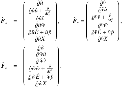$\begin{array}{ccc}\hat{{F}}\mathit{x}& \mathrm{=}& \left(\begin{array}{c}\\ \\ \\ \\ \\ \\ \end{array}\right)\mathit{,} \hat{{F}}\mathit{y}\mathrm{=}\left(\begin{array}{c}\\ \\ \\ \\ \\ \\ \end{array}\right)\mathit{,}\\ \hat{{F}}\mathit{z}& \mathrm{=}& \left(\begin{array}{c}\\ \\ \\ \\ \\ \\ \end{array}\right)\mathit{.}\end{array}$(3)They involve pressure that is related to the conservative variables by an equation of state.

These Euler equations express continuity of mass, balance of the components of momentum, balance of energy and, optionally, balance of scalar values. Note that the homogeneous Euler equations (i.e., S = 0) depend on a single, nondimensional reference quantity: the reference Mach number M_r = q_r/c_r. In the following, all quantities are nondimensional, and we drop the hat over the nondimensional quantities for convenience.

3. Fluid dynamics at low Mach numbers

In the limit of M → 0, the Euler equations (1) approach the incompressible equations of fluid dynamics, that is, the substantial derivative of the mass density, ∂ϱ/∂t + q·∇ϱ, vanishes. To show this, we follow the approach taken by Guillard & Viozat (1999) and expand the nondimensional quantities in terms of the reference Mach number, 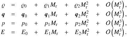$\begin{array}{ccc}\begin{array}{c}\\ & & & & & & & & \\ & & & & & & & & \\ & & & & & & & & \\ & & & & & & & & \end{array}& & \end{array}$(4)Each term in the expansions may be a function of space and time. For simplicity, we consider the homogeneous Euler equations (S = 0) in the following. With the above expressions, they read $\begin{array}{ccc}& & \frac{\mathit{\partial }}{\mathit{\partial t}}\hspace{0.17em}{\mathit{\varrho }}_{\mathrm{0}}\mathrm{+}\mathrm{\nabla }\mathrm{·}\left({\mathit{\varrho }}_{\mathrm{0}}{{q}}_{\mathrm{0}}\right)\mathrm{+}\mathrm{𝒪}\mathrm{\left(}{\mathit{M}}_{\mathrm{r}}\mathrm{\right)}\mathrm{=}\mathrm{0}\mathit{,}\\ & & \frac{\mathit{\partial }}{\mathit{\partial t}}\left({\mathit{\varrho }}_{\mathrm{0}}{{q}}_{\mathrm{0}}\right)\mathrm{+}\mathrm{\nabla }\mathrm{·}\left({\mathit{\varrho }}_{\mathrm{0}}{{q}}_{\mathrm{0}}\mathrm{\otimes }{{q}}_{\mathrm{0}}\right)\\ & & \mathrm{+}\hspace{0.17em}\frac{\mathrm{1}}{{\mathit{M}}_{\mathrm{r}}^{\mathrm{2}}}\mathrm{\nabla }{\mathit{p}}_{\mathrm{0}}\mathrm{+}\frac{\mathrm{1}}{{\mathit{M}}_{\mathrm{r}}}\mathrm{\nabla }{\mathit{p}}_{\mathrm{1}}\mathrm{+}\mathrm{\nabla }{\mathit{p}}_{\mathrm{2}}\mathrm{+}\mathrm{𝒪}\mathrm{\left(}{\mathit{M}}_{\mathrm{r}}\mathrm{\right)}\mathrm{=}\mathrm{0}\mathit{,}\\ & & \frac{\mathit{\partial }}{\mathit{\partial t}}\left({\mathit{\varrho }}_{\mathrm{0}}{\mathit{E}}_{\mathrm{0}}\right)\mathrm{+}\mathrm{\nabla }\mathrm{·}\left({\mathit{\varrho }}_{\mathrm{0}}{\mathit{E}}_{\mathrm{0}}{{q}}_{\mathrm{0}}\mathrm{+}{\mathit{p}}_{\mathrm{0}}{{q}}_{\mathrm{0}}\right)\mathrm{+}\mathrm{𝒪}\mathrm{\left(}{\mathit{M}}_{\mathrm{r}}\mathrm{\right)}\mathrm{=}\mathrm{0.}\end{array}$Obviously, terms in these equations scale differently with Mach number. To reach convergence in the limit of M → 0, it is necessary that the expressions of equal order in Mach number on the left-hand side vanish individually for the non-positive powers of M_r. We therefore find two simple relations, $\begin{array}{ccc}\mathrm{\nabla }{\mathit{p}}_{\mathrm{0}}\mathrm{=}\mathrm{\nabla }{\mathit{p}}_{\mathrm{1}}\mathrm{=}\mathrm{0}\mathit{,}& & \end{array}$(8)from the terms of order ${\mathit{M}}_{\mathrm{r}}^{-2}$ and ${\mathit{M}}_{\mathrm{r}}^{-1}$ in the momentum Eq. (6), respectively. Thus, pressure must be constant in space up to fluctuations of order ${\mathit{M}}_{\mathrm{r}}^{\mathrm{2}}$ (Guillard & Viozat 1999): $\begin{array}{ccc}\mathit{p}\mathrm{(}{x}\mathit{,}{\mathit{t}}^{\mathrm{)}}\mathrm{=}{\mathit{p}}_{\mathrm{0}}\mathrm{\left(}\mathit{t}\mathrm{\right)}\mathrm{+}{\mathit{p}}_{\mathrm{2}}\mathrm{\left(}{x}\mathit{,t}\mathrm{\right)}\hspace{0.17em}{\mathit{M}}_{\mathrm{r}}^{\mathrm{2}}\mathrm{+}\mathrm{𝒪}\mathrm{(}{{\mathit{M}}_{\mathrm{r}}^{\mathrm{3}}}^{\mathrm{)}}\mathit{.}& & \end{array}$(9)Time variations on the spatially constant p₀ can only be imposed through source terms, which we set to zero for the considerations in this article, or by the boundary conditions. In case of open boundary conditions, p₀ is set by the exterior pressure, which we assume to be temporally fixed following Guillard & Viozat (1999). Thus, p₀ is constant in space and time (see also Dellacherie 2010).

The expansion in Mach number is also applied to the equation of state. For simplicity, an ideal gas is assumed here. Inserting the expansion of the nondimensional quantities (4) into the nondimensionalized equation of state, $\begin{array}{ccc}\mathit{p}\mathrm{=}\mathrm{(}\mathit{\gamma }\mathrm{-}\mathrm{1}\mathrm{)}\left[\mathit{\varrho E}\mathrm{-}\frac{{\mathit{M}}_{\mathrm{r}}^{\mathrm{2}}}{\mathrm{2}}\mathit{\varrho }{\mathit{q}}^{\mathrm{2}}\right]\mathit{,}& & \end{array}$we obtain $\begin{array}{ccc}{\mathit{p}}_{\mathrm{0}}\mathrm{=}\mathrm{(}\mathit{\gamma }\mathrm{-}\mathrm{1}\mathrm{)}{\mathit{\varrho }}_{\mathrm{0}}{\mathit{E}}_{\mathrm{0}}\mathrm{+}\mathrm{𝒪}\mathrm{\left(}{\mathit{M}}_{\mathrm{r}}\mathrm{\right)}\mathit{.}& & \end{array}$(10)With Eqs. (8) and (10), the energy Eq. (7) can be transformed into $\begin{array}{ccc}\frac{\mathit{\partial }{\mathit{p}}_{\mathrm{0}}}{\mathit{\partial t}}\mathrm{+}\mathit{\gamma }{\mathit{p}}_{\mathrm{0}}\hspace{0.17em}\mathrm{\nabla }\mathrm{·}{{q}}_{\mathrm{0}}\mathrm{+}\mathrm{𝒪}\mathrm{\left(}{\mathit{M}}_{\mathrm{r}}\mathrm{\right)}\mathrm{=}\mathrm{0.}& & \end{array}$As argued above, p₀ is constant in time and thus the velocity field has to be divergence-free in zero Mach number limit, $\begin{array}{ccc}\mathrm{\nabla }\mathrm{·}{{q}}_{\mathrm{0}}\mathrm{=}\mathrm{0}\mathit{,}& & \end{array}$(11)recovering the incompressible flow when inserted into Eq. (5). We emphasize that according to Eq. (9), pressure fluctuations within the compressible Euler equations scale with the square of the reference Mach number as the solution convergences to a solution of the incompressible equations.

At the same time, however, stationary fluids with no mean velocity (i.e., at zero Mach number) can support the propagation of sound waves with arbitrarily small velocity fluctuations. We perform a standard linear stability analysis (e.g., Landau & Lifshitz 1959): for a fluid at rest with uniform mass density ϱ₀ = const. and pressure p₀ = const., deviations from this state can be expressed in terms of a small Mach number (M_r ≪ 1) following the expressions (4), except that in this case ϱ₀ and p₀ are independent of space and time. As before, we insert these expressions into the Euler Eqs. (1), but, in contrast to the analysis of the incompressible limit, we now keep terms up to order M_r. This results in $\begin{array}{ccc}\frac{\mathit{\partial }{\mathit{\varrho }}_{\mathrm{1}}}{\mathit{\partial t}}\mathrm{+}{\mathit{\varrho }}_{\mathrm{0}}\hspace{0.17em}\mathrm{\nabla }\mathrm{·}{{q}}_{\mathrm{1}}\mathrm{+}\mathrm{𝒪}\mathrm{\left(}{\mathit{M}}_{\mathrm{r}}\mathrm{\right)}\mathrm{=}\mathrm{0}& & \end{array}$for the continuity equation and $\begin{array}{ccc}{\mathit{\varrho }}_{\mathrm{0}}\frac{\mathit{\partial }{{q}}_{\mathrm{1}}}{\mathit{\partial t}}\mathrm{+}\frac{\mathrm{1}}{{\mathit{M}}_{\mathrm{r}}^{\mathrm{2}}}\mathrm{\nabla }{\mathit{p}}_{\mathrm{1}}\mathrm{+}\mathrm{𝒪}\mathrm{\left(}{\mathit{M}}_{\mathrm{r}}\mathrm{\right)}\mathrm{=}\mathrm{0}& & \end{array}$for the momentum equation. Instead of invoking the energy equation, we assume that pressure fluctuations result from reversible, adiabatic processes and thus express them in terms of mass density fluctuations using the nondimensional speed of sound: $\begin{array}{ccc}{\mathit{p}}_{\mathrm{1}}\mathrm{=}{\frac{\mathit{\partial p}}{\mathit{\partial \varrho }}|}_{\mathit{S}}\mathrm{·}{\mathit{\varrho }}_{\mathrm{1}}\mathrm{=}{\mathit{c}}^{\mathrm{2}}\mathrm{·}{\mathit{\varrho }}_{\mathrm{1}}\mathit{.}& & \end{array}$This transforms the continuity equation (dropping terms of order M_r) into $\begin{array}{ccc}\frac{\mathit{\partial }{\mathit{p}}_{\mathrm{1}}}{\mathit{\partial t}}\mathrm{+}{\mathit{\varrho }}_{\mathrm{0}}{\mathit{c}}^{\mathrm{2}}\hspace{0.17em}\mathrm{\nabla }\mathrm{·}{{q}}_{\mathrm{1}}\mathrm{=}\mathrm{0.}& & \end{array}$(12)Together with the momentum equation, we obtain a closed system for the evolution of q₁ and p₁. Introducing the velocity potential ψ, $\begin{array}{ccc}{{q}}_{\mathrm{1}}\mathrm{\equiv }\mathrm{\nabla }\mathit{\psi ,}& & \end{array}$we arrive at the linear wave equation $\begin{array}{ccc}\frac{{\mathit{\partial }}^{\mathrm{2}}\mathit{\psi }}{\mathit{\partial }{\mathit{t}}^{\mathrm{2}}}\mathrm{+}\frac{{\mathit{c}}^{\mathrm{2}}}{{\mathit{M}}_{\mathrm{r}}^{\mathrm{2}}}\hspace{0.17em}\mathrm{\Delta }\mathit{\psi }\mathrm{=}\mathrm{0}& & \end{array}$describing sound waves propagating at speed c/M_r. This derivation demonstrates that the Euler equations permit sound waves with arbitrarily small velocity fluctuations as solutions at arbitrarily small reference Mach numbers.

This result has important implications for the solutions of the compressible Euler equations at low Mach numbers: for sound waves, pressure fluctuations are on the same order in M_r as velocity fluctuations, as can be seen in Eq. (12). Thus, in contrast to the solutions approaching the incompressible regime discussed above, pressure fluctuations scale linearly with the reference Mach number, that is, 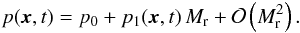$\begin{array}{ccc}\mathit{p}\mathrm{\left(}{x}\mathit{,t}\mathrm{\right)}\mathrm{=}{\mathit{p}}_{\mathrm{0}}\mathrm{+}{\mathit{p}}_{\mathrm{1}}\mathrm{\left(}{x}\mathit{,t}\mathrm{\right)}\hspace{0.17em}{\mathit{M}}_{\mathrm{r}}\mathrm{+}\mathrm{𝒪}\mathrm{(}{{\mathit{M}}_{\mathrm{r}}^{\mathrm{2}}}^{\mathrm{)}}\mathit{.}& & \end{array}$Sound waves are no solutions of the incompressible equations. Consequently, the compressible Euler equations permit two distinct classes of solutions in the limit of low Mach numbers: incompressible flows and sound waves. Schochet (1994) and Dellacherie (2010) proved that these types of solution decouple as the Mach number of the flow decreases.

This implies an important requirement for correct solutions of the compressible Euler equations in the regime of low Mach numbers:

Requirement 1. If the initial condition for the compressible, homogeneous Euler equations is chosen to be an incompressible flow (i.e., it is “well-prepared” such that pressure fluctuations scale with ${\mathit{M}}_{\mathrm{r}}^{\mathrm{2}}$ ), then the solution must stay in the incompressible regime.

This requirement holds for continuous solutions. At the same time, it is an important quality criterion for numerical schemes not to violate this constraint. For this, an appropriate discretization is necessary, as we discuss in Sects. 7 and 8.

Another constraint results from considering the evolution of kinetic energy. Its density, ${\mathit{ϵ}}_{\mathrm{kin}}\mathrm{=}\frac{\mathrm{1}}{\mathrm{2}}\mathit{\varrho }{\mathit{q}}^{\mathrm{2}}$, is usually treated as part of the total energy ϱE in the Euler equations. However, a separate evolution equation for the kinetic energy can be derived from Eq. (1)in the case of vanishing source terms in the equations of mass and momentum conservation: $\begin{array}{ccc}\frac{\mathit{\partial }{\mathit{ϵ}}_{\mathrm{kin}}}{\mathit{\partial t}}\mathrm{+}\mathrm{\nabla }\mathrm{·}\left[\left({\mathit{ϵ}}_{\mathrm{kin}}\mathrm{+}\frac{\mathit{p}}{{\mathit{M}}_{\mathrm{r}}^{\mathrm{2}}}\right){q}\right]\mathrm{=}\frac{\mathit{p}}{{\mathit{M}}_{\mathrm{r}}^{\mathrm{2}}}\mathrm{\nabla }\mathrm{·}{q}\mathit{.}& & \end{array}$This equation is in strong conservation form, except for the source term on the right-hand side. However, since the velocity divergence vanishes for incompressible flows, we identify another requirement for the correct solution in the low Mach number regime:

Requirement 2. For solutions to the compressible, homogeneous Euler equations in the limit of low Mach numbers, the total kinetic energy is conserved.

This implies that no dissipation takes place and establishes another quality criterion for numerical discretization.

The two requirements pose severe challenges to a numerical treatment of flows at low Mach numbers with conventional Godunov-type solvers. Such approaches cannot guarantee the correct asymptotic behavior because their solution strategy conflicts with the well-preparedness of the initial condition in each time step. The idea of Godunov-like schemes is to advance the hydrodynamic states by discretizing the conserved quantities in a way that discontinuities appear at the cell interfaces. This defines Riemann problems for which an analytic solution is known (in practical implementations, approximate solutions are constructed) so that the hydrodynamical fluxes over the cell edges can be determined. The introduction of discontinuities and the wave pattern resulting from the solution to the Riemann problem, however, is incompatible with flows at low Mach numbers near the incompressible regime. This is illustrated and further discussed in Sect. 7. In addition to this fundamental problem, we encounter a practical problem for the numerical discretization. In the limit of low Mach numbers, the fluid velocity is orders of magnitude lower than the sound speed. This disparity of scales leads to a stiffness of the system of equations to be solved.

Although requirements 3 and 3 are not easy to fulfill in the discretized version, it still appears worthwhile to begin from the compressible equations of fluid dynamics. In contrast to other methods, no a priori approximations enter the basic equations. Therefore, schemes based on this approach promise to be applicable in flow regimes covering a wide range of Mach numbers, from incompressible flows over moderate Mach numbers to the supersonic regime. In the following, we examine the behavior of a widely used Godunov-like scheme based on the solver suggested by Roe (1981). We propose a modification to this scheme, which ensures correct low-Mach-number scaling and also alleviates the stiffness problems. The appeal of this approach is that it retains the advantages of conventional Godunov-type solvers of the compressible equations of hydrodynamics, such as flexibility of application and high efficiency, while allowing for modeling flow regimes that were inaccessible without the proposed modifications.

4. Testbed: the Gresho vortex problem

Before discussing the properties of numerical hydrodynamics solvers in more detail, we set out a test problem that illustrates the problems of conventional schemes and allows us to demonstrate the advantages of the proposed modifications. A suitable setup is a rotating flow in form of the Gresho vortex (Gresho & Chan 1990). This vortex is a time-independent solution of the incompressible, homogeneous Euler equations where centrifugal forces are exactly balanced by pressure gradients. It was first applied to the compressible Euler equations by Liska & Wendroff (2003).

The problem is set up in a two-dimensional box. For nondimensionalization, we choose the reference length x_r to equal the domain size, so that the spatial coordinates x and y extend over [ 0,1 ] with periodic boundary conditions. This domain is filled with an ideal gas of constant mass density, which sets our reference mass density, that is, ϱ(x,y) = const. = ϱ_r.

The rotation of the vortex, which is centered at (x,y) = (0.5,0.5), is initiated by imposing a simple angular velocity distribution of 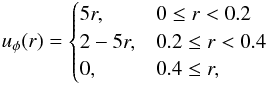$\begin{array}{ccc}{\mathit{u}}_{\mathit{\phi }}\mathrm{\left(}\mathit{r}\mathrm{\right)}\mathrm{=}\{\begin{array}{c}\\ & \\ & \\ & \end{array}& & \end{array}$given in units of the reference fluid velocity q_r. Here, $\mathit{r}\mathrm{=}\sqrt{{\left(\mathit{x}\mathrm{-}\mathrm{0.5}\right)}^{\mathrm{2}}\mathrm{+}{\left(\mathit{y}\mathrm{-}\mathrm{0.5}\right)}^{\mathrm{2}}}$ denotes the radial coordinate of the rotating flow. The velocity reaches its maximum value u_φ,max = 1 at r = 0.2. For convenience, we arrange the reference time, t_r, to equal the period of the vortex. This is achieved by setting the reference velocity to $\begin{array}{ccc}{\mathit{q}}_{\mathrm{r}}\mathrm{=}\frac{\mathrm{0.4}\mathit{\pi }{\mathit{x}}_{\mathrm{r}}}{{\mathit{t}}_{\mathrm{r}}}\mathrm{·}& & \end{array}$To stabilize the flow, we set the pressure such that its gradient gives rise to the required centripetal force: $\begin{array}{ccc}\mathit{p}\mathrm{\left(}\mathit{r}\mathrm{\right)}\mathrm{=}\{\begin{array}{c}\\ & \\ & \\ & \end{array}& & \end{array}$(13)This pressure profile is arranged to be continuous and differentiable everywhere and has a free constant p₀. We use this parameter to conveniently adjust the maximum Mach number of the problem. The Mach number $\begin{array}{ccc}\mathit{M}\mathrm{\left(}\mathit{r}\mathrm{\right)}\mathrm{=}\frac{{\mathit{u}}_{\mathit{\phi }}\mathrm{\left(}\mathit{r}\mathrm{\right)}}{\sqrt{\mathit{\gamma p}\mathrm{\left(}\mathit{r}\mathrm{\right)}\mathit{/}{\mathit{\varrho }}_{\mathrm{0}}}}& & \end{array}$reaches its maximum, M_max, at r = 0.2. Depending on the intended maximum Mach number of the vortex flow, we set the pressure parameter to $\begin{array}{ccc}{\mathit{p}}_{\mathrm{0}}\mathrm{=}\frac{{\mathit{\varrho }}_{\mathrm{0}}\hspace{0.17em}{\mathit{u}}_{\mathit{\phi ,}\max }^{\mathrm{2}}}{\mathit{\gamma }{\mathit{M}}_{\max }^{\mathrm{2}}}\mathrm{-}\frac{\mathrm{1}}{\mathrm{2}}\mathrm{·}& & \end{array}$(14)We note that setting the reference Mach number M_r = M_max implies that p_r = p₀.

When choosing p₀ as in Eq. (14), it follows from Eq. (13) that pressure fluctuations scale with the square of the Mach number, $\begin{array}{ccc}\frac{\mathit{p}\mathrm{-}{\mathit{p}}_{\mathrm{0}}}{{\mathit{p}}_{\mathrm{0}}}\mathrm{\propto }{\mathit{M}}_{\max }^{\mathrm{2}}\mathit{.}& & \end{array}$Thus, according to the discussion in Sect. 3, the initial condition is well prepared, meaning that the flow is in the incompressible regime and no sound waves occur. The Gresho vortex as set up here is a stationary solution to the incompressible Euler equations and thus should not change with time. Any deviations from stationarity observed in its evolution can be attributed to discretization errors of the applied numerical scheme. We therefore use this problem to check the quality of hydro solvers in the regime of low Mach numbers.

We emphasize that although the Gresho vortex problem is a simplistic setup, it still provides a relevant test for realistic applications of numerical hydro-solvers. While discretization errors can usually be alleviated with higher spatial resolution, complex flows as encountered in many astrophysical situations still pose problems. In particular for turbulent flows, a higher resolution of the domain will usually reveal smaller-scale structures near the cutoff at the grid scale. These are again poorly resolved, and discretization errors are most pronounced here. The quality of a numerical scheme for modeling flows at low Mach numbers reflects this in its ability to adequately represent such structures. In our Gresho vortex testbed, we therefore intentionally chose a discretization of the domain in only 40 × 40 grid cells.

The initial setup of the Gresho vortex outlined above is shown in Fig. 1. It is advanced in time from t = 0.0 to t = 1.0, corresponding to one full revolution of the vortex. The choice of the time discretization method has only a minor effect on the results of our tests. As a standard for the examples shown below, we chose the implicit, third-order Runge–Kutta method ESDIRK34 (Kennedy & Carpenter 2001). Because of the integrated error estimator of this method, adaptive time-step control might be used in principle. However, we instead employed an advective CFL criterion to determine the time step size Δt, $\begin{array}{ccc}\mathrm{\Delta }\mathit{t}\mathrm{=}\frac{{\mathit{c}}_{\mathrm{CFL}}}{{\mathit{N}}_{\dim }\min \left(\frac{\mathrm{\Delta }}{\mathrm{\left|}{\mathit{q}}_{\mathit{n}}\mathrm{\right|}}\right)}\mathit{,}& & \end{array}$(15)where the CFL factor is set to c_CFL = 0.5, and the number of spatial dimensions of our problem is N_dim = 2. Δ and q_n are the width of the computational cell and the magnitude of the normal velocity, see Sect. 5. This implicit method is particularly well suited for our purposes. At low Mach numbers, its numerical efficiency is expected to be higher than that of explicit schemes. Moreover, it allows evolving the problem at various Mach numbers over a given physical time with the same number of numerical time steps. This increases the comparability between the runs because potential numerical dissipation due to temporal discretization is kept constant.

However, to substantiate our claim that the success of our new method for simulating flows at low Mach numbers be independent of the employed temporal discretization, we also ran some test problems with the time-explicit RK3 scheme of Shu & Osher (1988). Implementation details and efficiency tests of the temporal discretization will be presented in a forthcoming publication.

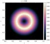Fig. 1 Setup of the Gresho vortex problem for Mmax = 0.1. The Mach number is color coded.

5. Spatial discretization

Our approach to modeling flows at low Mach numbers is based on the compressible Euler equations and uses standard discretization methods. Here, we discuss the spatial discretization of the equations by following the method of lines (e.g., Toro 2009) to arrive at a semi-discrete scheme. We perform a finite-volume discretization starting from the Euler Eqs. (1), 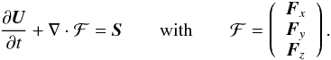$\begin{array}{ccc}\frac{\mathit{\partial }{U}}{\mathit{\partial t}}\mathrm{+}\mathrm{\nabla }\mathrm{·}\mathrm{ℱ}\mathrm{=}{S}\mathrm{with}\mathrm{ℱ}\mathrm{=}\left(\begin{array}{c}\\ \\ \\ \end{array}\right)\mathit{.}& & \end{array}$(16)For simplicity and clarity of notation, we use a general flux vector F instead of writing out its Cartesian components in the following. This general form can be expressed in terms of the normal velocity q_n, its magnitude q_n, and its normalized, Cartesian components n_x, n_y, and n_z: $\begin{array}{ccc}{F}\mathrm{=}\left(\begin{array}{c}\\ \\ \\ \\ \\ \end{array}\right)\mathit{.}& & \end{array}$(17)For instance, for the flux in x-direction of Cartesian coordinates we have q_n = (u,0,0)^⊤, q_n = u and n_x = 1, n_y = 0, n_z = 0. This results in the expression for F_x as in Eq. (3).

Spatial discretization is performed in Cartesian coordinates by partitioning the domain of interest into a regular, equidistant grid of N_x × N_y × N_z cells. This has the advantage that the cell widths are uniform, that is, Δx = Δy = Δz = Δ, simplifying some of the further expressions. However, an equidistant grid is not required, and the expressions given below can be easily generalized. Integer values of the coordinates refer to cell centers, for instance, (i,j,k). Cell faces are denoted by half integer values in the corresponding direction. For example, the interface between cell i and cell i + 1 in the x-direction is marked with i + 1/2.

Integration of (16) over the volume Ω_i,j,k of a cell (i,j,k) gives 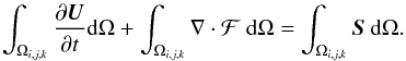$\begin{array}{ccc}{\mathrm{\int }}_{{\mathrm{\Omega }}_{\mathit{i,j,k}}}\frac{\mathit{\partial }{U}}{\mathit{\partial t}}\mathrm{d\Omega }\mathrm{+}{\mathrm{\int }}_{{\mathrm{\Omega }}_{\mathit{i,j,k}}}\mathrm{\nabla }\mathrm{·}\mathrm{ℱ}\mathrm{d\Omega }\mathrm{=}{\mathrm{\int }}_{{\mathrm{\Omega }}_{\mathit{i,j,k}}}{S}\mathrm{d\Omega }\mathit{.}& & \end{array}$The first term on the left-hand side is the time derivative of the integral of the conserved variables over a cell of volume V_i,j,k. We thus introduce cell-averaged quantities: 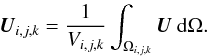$\begin{array}{ccc}{{U}}_{\mathit{i,j,k}}\mathrm{=}\frac{\mathrm{1}}{{\mathit{V}}_{\mathit{i,j,k}}}{\mathrm{\int }}_{{\mathrm{\Omega }}_{\mathit{i,j,k}}}{U}\mathrm{d\Omega }\mathit{.}& & \end{array}$The source term on the right-hand side of the equation is treated analogously, and we arrive at $\begin{array}{ccc}\frac{\mathit{\partial }{{U}}_{\mathit{i,j,k}}}{\mathit{\partial t}}\mathrm{+}\frac{\mathrm{1}}{{\mathit{V}}_{\mathit{i,j,k}}}{\mathrm{􏽉}}_{\mathit{\partial }\mathrm{\Omega }}\mathrm{ℱ}\mathrm{·}{n}\mathrm{d𝒮}\mathrm{=}{{S}}_{\mathit{i,j,k}}\mathit{.}& & \end{array}$The surface integral is discretized by defining numerical fluxes from the integrated fluxes through the six surfaces of the three dimensional cell (i,j,k): $\begin{array}{ccc}{{F}}_{\mathit{i}\mathrm{+}\mathrm{1}\mathit{/}\mathrm{2}\mathit{,j,k}}& \mathrm{=}& 􏽉\mathit{\partial }\mathrm{\Omega }\mathrm{(}\mathit{i}\mathrm{+}\mathrm{1}\mathit{/}\mathrm{2}\mathit{,j,k}\mathrm{)}{{F}}_{\mathit{x}}\mathrm{d𝒮}\mathit{,}\\ {{F}}_{\mathit{i}\mathrm{-}\mathrm{1}\mathit{/}\mathrm{2}\mathit{,j,k}}& \mathrm{=}& 􏽉\mathit{\partial }\mathrm{\Omega }\mathrm{(}\mathit{i}\mathrm{-}\mathrm{1}\mathit{/}\mathrm{2}\mathit{,j,k}\mathrm{)}{{F}}_{\mathit{x}}\mathrm{d𝒮}\mathit{,}\\ {{F}}_{\mathit{i,j}\mathrm{+}\mathrm{1}\mathit{/}\mathrm{2}\mathit{,k}}& \mathrm{=}& 􏽉\mathit{\partial }\mathrm{\Omega }\mathrm{(}\mathit{i,j}\mathrm{+}\mathrm{1}\mathit{/}\mathrm{2}\mathit{,k}\mathrm{)}{{F}}_{\mathit{y}}\mathrm{d𝒮}\mathit{,}\\ {{F}}_{\mathit{i,j}\mathrm{-}\mathrm{1}\mathit{/}\mathrm{2}\mathit{,k}}& \mathrm{=}& 􏽉\mathit{\partial }\mathrm{\Omega }\mathrm{(}\mathit{i,j}\mathrm{-}\mathrm{1}\mathit{/}\mathrm{2}\mathit{,k}\mathrm{)}{{F}}_{\mathit{y}}\mathrm{d𝒮}\mathit{,}\\ {{F}}_{\mathit{i,j,k}\mathrm{+}\mathrm{1}\mathit{/}\mathrm{2}}& \mathrm{=}& 􏽉\mathit{\partial }\mathrm{\Omega }\mathrm{(}\mathit{i,j,k}\mathrm{+}\mathrm{1}\mathit{/}\mathrm{2}\mathrm{)}{{F}}_{\mathit{z}}\mathrm{d𝒮}\mathit{,}\\ {{F}}_{\mathit{i,j,k}\mathrm{-}\mathrm{1}\mathit{/}\mathrm{2}}& \mathrm{=}& {\mathrm{􏽉}}_{\mathit{\partial }\mathrm{\Omega }\mathrm{(}\mathit{i,j,k}\mathrm{-}\mathrm{1}\mathit{/}\mathrm{2}\mathrm{)}}{{F}}_{\mathit{z}}\mathrm{d𝒮}\mathit{.}\end{array}$(18)This results in the semi-discrete version of the Euler equations, $\begin{array}{ccc}\frac{\mathit{\partial }}{\mathit{\partial t}}{{U}}_{\mathit{i,j,k}}& \mathrm{+}& \mathrm{(}{\mathit{V}}_{\mathit{i,j,k}}{\mathrm{)}}^{-1}({{F}}_{\mathit{i}\mathrm{+}\mathrm{1}\mathit{/}\mathrm{2}\mathit{,j,k}}\mathrm{-}{{F}}_{\mathit{i}\mathrm{-}\mathrm{1}\mathit{/}\mathrm{2}\mathit{,j,k}}\mathrm{+}{{F}}_{\mathit{i,j}\mathrm{+}\mathrm{1}\mathit{/}\mathrm{2}\mathit{,k}}\\ & \mathrm{-}& {{F}}_{\mathit{i,j}\mathrm{-}\mathrm{1}\mathit{/}\mathrm{2}\mathit{,k}}\mathrm{+}{{F}}_{\mathit{i,j,k}\mathrm{+}\mathrm{1}\mathit{/}\mathrm{2}}\mathrm{-}{{F}}_{\mathit{i,j,k}\mathrm{-}\mathrm{1}\mathit{/}\mathrm{2}})\mathrm{=}{{S}}_{\mathit{i,j,k}}\mathit{.}\end{array}$(19)At the domain edges, boundary conditions must be implemented either by introducing layers of ghost cells or by local modification of the discretization scheme (see, e.g., Toro 2009).

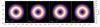Fig. 2 Gresho vortex problem advanced to t = 1.0 with a central flux discretization scheme for different maximum Mach numbers Mmax in the setup, as indicated in the plots. The Mach number relative to the respective Mmax is color coded.

6. Numerical flux functions

The key ingredient in any finite-volume scheme is constructing the numerical fluxes defined in Eq. (18). The discretization described above stores cell-averaged quantities at the cell centers. According to Eq. (19), these quantities are evolved in time by computing numerical fluxes over the cell interfaces. These, in turn, are obtained from the state variables, and thus their cell-centered values have to be interpolated to interface-centered values by appropriate reconstruction methods. Here, standard schemes are employed, and we refer to the literature for further details (e.g., Toro 2009). For the test problems below, we always used a piecewise linear, MUSCL-like reconstruction (van Leer 1979; Toro 2009) without any limiter because our tests only involve smooth problems². The low-Mach-number methods we focus on here, however, only modify the flux function and can thus be combined with any kind of reconstruction. In fact, the improvement is even more significant for low-order schemes because low-Mach inconsistencies in the flux function are even more pronounced here.

6.1. Central flux

Interpolations to interface-centered values, for instance at the interface l + 1/2, with l ∈ { i,j,k }, carried out separately from both (“left” and “right”) sides result in different values, denoted by ${{U}}_{\mathit{l}\mathrm{+}\mathrm{1}\mathit{/}\mathrm{2}}^{\mathit{L}}$ and ${{U}}_{\mathit{l}\mathrm{+}\mathrm{1}\mathit{/}\mathrm{2}}^{\mathit{R}}$³.

A straightforward approach would be to use central fluxes, 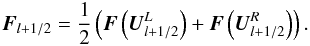$\begin{array}{ccc}{{F}}_{\mathit{l}\mathrm{+}\mathrm{1}\mathit{/}\mathrm{2}}\mathrm{=}\frac{\mathrm{1}}{\mathrm{2}}\mathrm{(}{F}\mathrm{(}{{{U}}_{\mathit{l}\mathrm{+}\mathrm{1}\mathit{/}\mathrm{2}}^{\mathit{L}}}^{\mathrm{)}}\mathrm{+}{F}{\mathrm{(}{{{U}}_{\mathit{l}\mathrm{+}\mathrm{1}\mathit{/}\mathrm{2}}^{\mathit{R}}}^{\mathrm{)}}}^{\mathrm{)}}\mathit{.}& & \end{array}$(20)As an illustration, we solve the Gresho vortex problem (see Sect. 4) with a central flux scheme. The flow at t = 1 (corresponding to one full revolution of the vortex) is shown in Fig. 2. Remarkably, it looks almost identical to the setup at t = 0 (see Fig. 1), even for low values of the maximum Mach number.

However, the scheme resulting from central fluxes is known to be numerically unstable for many explicit time-discretization schemes. In our numerical tests with implicit time discretization, problems arise in the evolution of the total kinetic energy of the flow, as shown in Fig. 3. The observed increase is unphysical. Discretization errors continue to grow with time, and therefore a central flux function cannot be used for practical implementations. Generally, to achieve stability in the numerical solution of hyperbolic equations, some kind of upwinding mechanism is necessary. Still, the central-flux method is instructive for constructing solvers for low Mach numbers, as we describe below.

Fig. 3 Temporal evolution of the total kinetic energy Ekin(t) relative to its initial value Ekin(0) in the Gresho vortex problem advanced with central fluxes. The cases for Mmax = 10-1, 10-2, 10-3, and 10-4 are overplotted but are virtually indistinguishable.

6.2. Godunov schemes and Roe flux

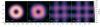Fig. 4 Gresho vortex problem advanced to t = 1.0 with the Roe flux discretization scheme for different maximum Mach numbers Mmax in the setup, as indicated in the plots. The Mach number relative to the respective Mmax is color coded.

One way to achieve stability of numerical schemes is to employ Godunov-like methods (Godunov 1959) for computing numerical fluxes. Neglecting source terms, the reconstructed values at cell interfaces pose one-dimensional Riemann problems: at interface l + 1/2 we have $\begin{array}{ccc}\frac{\mathit{\partial }{U}}{\mathit{\partial t}}\mathrm{+}\frac{\mathit{\partial }{{F}}_{\mathit{\xi }}}{\mathit{\partial \xi }}\mathrm{=}\mathrm{0}& & \end{array}$(21)with the initial condition $\begin{array}{ccc}{U}\left(\mathit{\xi ,t}\mathrm{=}\mathrm{0}\right)\mathrm{=}\{\begin{array}{c}\\ \\ \end{array}& & \end{array}$(22)The coordinate ξ is measured relative to the cell interface and along the Cartesian direction x, y, or z that corresponds to l ∈ { i,j,k }. The analytic solution to this Riemann problem is self-similar, $\begin{array}{ccc}{U}\left(\mathit{\xi ,t}\right)\mathrm{=}{{U}}^{\mathrm{\ast }}\left(\mathit{\xi }\mathit{/}\mathit{t}\right)\mathit{,}& & \end{array}$and can be used to define a numerical flux function, $\begin{array}{ccc}{{F}}_{\mathit{l}\mathrm{+}\mathrm{1}\mathit{/}\mathrm{2}}\mathrm{=}{F}\left[{{U}}^{\mathrm{\ast }}\mathrm{(}{\mathrm{0}}^{\mathrm{)}}\right]\mathit{,}& & \end{array}$over the cell interface l + 1/2 in ξ-direction.

Riemann problems can be solved exactly, but because of inevitable discretization errors, an approximate solution is usually sufficient and reduces the computational effort significantly. A very popular approximate Riemann solver was developed by Roe (1981). It is based on a local linearization of Eq. (21), $\begin{array}{ccc}\frac{\mathit{\partial }{U}}{\mathit{\partial t}}\mathrm{+}\frac{\mathit{\partial }{{F}}_{\mathit{\xi }}}{\mathit{\partial \xi }}\mathrm{=}\frac{\mathit{\partial }{U}}{\mathit{\partial t}}\mathrm{+}{A}\mathrm{\left(}{U}\mathrm{\right)}\frac{\mathit{\partial }{U}}{\mathit{\partial \xi }}\mathrm{=}\mathrm{0}\mathit{,}& & \end{array}$which is achieved by replacing the flux Jacobian matrix $\begin{array}{ccc}{A}\mathrm{\left(}{U}\mathrm{\right)}\mathrm{\equiv }\frac{\mathit{\partial }{{F}}_{\mathit{\xi }}}{\mathit{\partial }{U}}& & \end{array}$with a constant matrix A${}_{\mathrm{roe}}\mathrm{\left(}{{U}}_{\mathit{l}\mathrm{+}\mathrm{1}\mathit{/}\mathrm{2}}^{\mathit{L}}\mathit{,}{{U}}_{\mathit{l}\mathrm{+}\mathrm{1}\mathit{/}\mathrm{2}}^{\mathit{R}}\mathrm{\right)}$. This transforms the original Riemann problem (21,22) into a linear system with constant coefficients while leaving the initial conditions unaltered. The flux function for this modified system is given by (e.g., Toro 2009) $\begin{array}{ccc}{{F}}_{\mathit{l}\mathrm{+}\mathrm{1}\mathit{/}\mathrm{2}}& \mathrm{=}& \frac{\mathrm{1}}{\mathrm{2}}\mathrm{[}{F}\mathrm{(}{{{U}}_{\mathit{l}\mathrm{+}\mathrm{1}\mathit{/}\mathrm{2}}^{\mathit{L}}}^{\mathrm{)}}\mathrm{+}{F}{\mathrm{(}{{{U}}_{\mathit{l}\mathrm{+}\mathrm{1}\mathit{/}\mathrm{2}}^{\mathit{R}}}^{\mathrm{)}}}^{}\\ & & \mathrm{-}\left|{{A}}_{\mathrm{roe}}\right|{\mathrm{(}{{U}}_{\mathit{l}\mathrm{+}\mathrm{1}\mathit{/}\mathrm{2}}^{\mathit{R}}\mathrm{-}{{{U}}_{\mathit{l}\mathrm{+}\mathrm{1}\mathit{/}\mathrm{2}}^{\mathit{L}}}^{\mathrm{)}}}^{\mathrm{]}}\mathit{.}\end{array}$(23)This expression is used as an approximation to the flux function of the original nonlinear Riemann problem. To this end, the constant matrix A_roe has to be specified. Generally, the flux Jacobian matrix A can be decomposed into a set of right eigenvectors R and a diagonal matrix $\begin{array}{ccc}{\Lambda }\mathrm{=}\mathrm{diag}\left({\mathit{q}}_{\mathit{n}}\mathrm{-}\frac{\mathrm{1}}{{\mathit{M}}_{\mathrm{r}}}\mathit{c,}{\mathit{q}}_{\mathit{n}}\mathrm{+}\frac{\mathrm{1}}{{\mathit{M}}_{\mathrm{r}}}\mathit{c,}{\mathit{q}}_{\mathit{n}}\mathit{,}{\mathit{q}}_{\mathit{n}}\mathit{,}{\mathit{q}}_{\mathit{n}}\mathit{,}{\mathit{q}}_{\mathit{n}}\right)\mathit{,}& & \end{array}$(24)containing the corresponding eigenvalues, so that $\begin{array}{ccc}{A}\mathrm{=}{R}{\Lambda }{{R}}^{-1}\mathit{.}& & \end{array}$(25)To determine |A_roe|, this matrix and its absolute value, $\begin{array}{ccc}\left|{A}\right|\mathrm{\equiv }{R}\left|{\Lambda }\right|{{R}}^{-1}\mathit{,}& & \end{array}$(26)are evaluated at the so-called Roe-averaged state. Roe (1981) set out three requirements for its construction. The most important of them, $\begin{array}{ccc}{F}\mathrm{(}{{U}}^{\mathit{R}}\mathrm{)}\mathrm{-}{F}\mathrm{(}{{U}}^{\mathit{L}}\mathrm{)}\mathrm{=}{{A}}_{\mathrm{roe}}\mathrm{(}{{U}}^{\mathit{R}}\mathrm{-}{{U}}^{\mathit{L}}\mathrm{)}\mathit{,}& & \end{array}$(27)ensures conservation across discontinuities.

With the three requirements, however, a unique Roe-averaged state can only be derived for ideal gases. For a general equation of state, such as needed for astrophysical applications, a number of extensions to the original Roe scheme have been proposed (see, e.g., Vinokur & Montagné 1990; Mottura et al. 1997; Cinnella 2006).

In Eq. (23) | A_roe | was introduced from the solution of a (linearized) Riemann problem at the cell interface. However, it can be interpreted in a slightly different fashion. Comparing expression (23) with the central flux (20), we note that the term involving | A_roe | acts to balance the numerical flux function either toward the left or right approaching state, depending on the characteristic decomposition and its eigenvalues. It thus enforces that the characteristic waves are discretized at the upwind state of the fluid. This is essential for the numerical stability of the scheme.

If, for example, the flow is supersonic in the corresponding positive coordinate direction, all eigenvalues (24)are positive. Since, by construction of A_roe relation (27) holds, the resulting numerical flux is ${{F}}_{\mathit{l}\mathrm{+}\mathrm{1}\mathit{/}\mathrm{2}}\mathrm{=}{F}{}^{\mathrm{\right(}}{{U}}_{\mathit{l}\mathrm{+}\mathrm{1}\mathit{/}\mathrm{2}}^{\mathit{L}}^{\mathrm{\left)}}$ and the other terms in (23) cancel out. For subsonic flows, the numerical flux is a sum of terms resulting from discretizing each characteristic wave in the upwind direction.

More generally, the numerical flux function of any Godunov-like scheme can be expressed in quasi-linear form by $\begin{array}{ccc}{{F}}_{\mathit{l}\mathrm{+}\mathrm{1}\mathit{/}\mathrm{2}}\mathrm{=}\frac{\mathrm{1}}{\mathrm{2}}\mathrm{[}{{A}}^{\mathit{L}}{{U}}_{\mathit{l}\mathrm{+}\mathrm{1}\mathit{/}\mathrm{2}}^{\mathit{L}}\mathrm{+}{{A}}^{\mathit{R}}{{U}}_{\mathit{l}\mathrm{+}\mathrm{1}\mathit{/}\mathrm{2}}^{\mathit{R}}\mathrm{-}{D}{\mathrm{(}{{U}}_{\mathit{l}\mathrm{+}\mathrm{1}\mathit{/}\mathrm{2}}^{\mathit{R}}\mathrm{-}{{{U}}_{\mathit{l}\mathrm{+}\mathrm{1}\mathit{/}\mathrm{2}}^{\mathit{L}}}^{\mathrm{)}}}^{\mathrm{]}}\mathit{,}& & \end{array}$(28)where D is an “upwinding matrix”. The corresponding term in the flux is introduced as a numerical measure to stabilize the scheme by ensuring flux evaluation in upwind direction. When inserted into the semi-discrete version of the Euler Eqs. (19), however, it gives rise to the discretized form of a second space derivative of the state vector. Thus, it acts as a viscosity, and therefore the corresponding term is sometimes also called “upwind artificial viscosity” (Guillard & Murrone 2004). It is clear that it must not dominate the physical flux represented by the terms involving A^L and A^R. This is the problem encountered for D = | A_roe | at low Mach numbers, as we discuss in Sect. 7.

We again tested the performance of Roe’s approach to model the hydrodynamic fluxes by solving the Gresho problem. The result is shown in Fig. 4. The effect of dissipation is obvious already for moderately low Mach numbers. After a full revolution, the Mach number of the flow has decreased and the vortex does not appear as crisp as in the setup and in the cases with central fluxes (cf. Fig. 2). With lower Mach numbers the dissipation increases strongly, and already at M_max ≲ 10^-3 the vortex is completely dissolved before completing one revolution.

This behavior can be quantified by the loss of kinetic energy of the flows, as given in the first row of Table 1 (“not preconditioned”). Although the scheme based on Roe’s numerical fluxes is stable (in contrast to the case of central fluxes where the kinetic energy increases unphysically), it violates requirement 3 of Sect. 3. The asymptotic behavior of the Euler equations requires the kinetic energy to be exactly conserved in the zero-Mach number limit. Therefore, the excessive dissipation of the Roe scheme for low Mach numbers is attributed to artificial dissipation inherent to the discretization.

The failure to reproduce incompressible flow fields is well known in the fluid dynamics literature (e.g., Volpe 1993; Guillard & Viozat 1999) and not unique to the particular choice of Roe’s numerical flux function. Instead, Guillard & Murrone (2004) showed that it is fundamentally inherent to the Godunov solution strategy. They examined the scaling behavior of the pressure p^∗ at cell interfaces by an expansion of the Riemann problem for the nondimensional Euler equations in terms of reference Mach number, similar to the approach discussed in Sect. 3 (see Eq. (4)). This pressure of the self-similar solution to the Riemann problem then takes the form (Guillard & Murrone 2004) $\begin{array}{ccc}{\mathit{p}}^{\mathrm{\ast }}\mathrm{=}{\mathit{\varrho }}_{\mathrm{r}}{\mathit{c}}_{\mathrm{r}}^{\mathrm{2}}\left({\mathit{p}}_{\mathrm{0}}\mathrm{-}\frac{\mathrm{1}}{\mathrm{2}}{\mathit{M}}_{\mathrm{r}}\sqrt{\mathit{\gamma }{\mathit{p}}_{\mathrm{0}}{\mathit{\varrho }}_{\mathrm{0}}}\mathrm{\Delta }{\mathit{u}}_{\mathrm{1}}\mathrm{+}\mathrm{·}\mathrm{·}\mathrm{·}\hspace{0.17em}\right)\mathit{.}& & \end{array}$(29)Obviously, this is in conflict with the scaling behavior in the regime of low Mach numbers discussed in Sect. 3: the pressure in incompressible flows must be constant in space and time, up to fluctuations that scale with the square of the reference Mach number. In contrast, p^∗ contains fluctuations that scale linearly with M_r, as is characteristic for sound waves. These sound waves are produced by the first-order velocity jump Δu₁ over the interface. Therefore, classical Godunov-like schemes are inconsistent with requirement 3 of Sect. 3.

The fact that an incompressible solution cannot be maintained by standard Godunov-like methods does not come as a surprise. We recall that jumps in the flow variables are intentionally created at the cell interfaces by the Godunov discretization strategy in order to define Riemann problems that can easily be solved. This is in conflict with the smooth flow-fields in the incompressible regime. The artificial introduction of discontinuities leads to the generation of artificial sound waves, which are not resolved on the grid and quickly get dissipated. This provides a heuristic argument for the excessive dissipation of the schemes at low Mach numbers. It may therefore be argued that the Godunov approach is unsuited for modeling flows at low Mach numbers. However, for reasons given in Sect. 3, such schemes are still attractive for a numerical simulation of astrophysical problems. As a measure to salvage conventional solvers, preconditioning techniques for the numerical flux functions have been proposed (see Turkel 1999, for a review), and we investigate this approach in the following.

7. Low-Mach-number scaling of Godunov-type numerical flux functions

The differences in the low-Mach-number behavior observed in the central flux and the Roe schemes indicate the origin of the excessive dissipation in the latter. Comparing the flux functions of the central scheme (20) to that of Roe (23), or, more generally, to the flux function of any Godunov-like scheme (28), we suspect the respective upwinding terms $\begin{array}{ccc}\left|{{A}}_{\mathrm{roe}}\right|\mathrm{(}{{U}}_{\mathit{l}\mathrm{+}\mathrm{1}\mathit{/}\mathrm{2}}^{\mathit{R}}\mathrm{-}{{{U}}_{\mathit{l}\mathrm{+}\mathrm{1}\mathit{/}\mathrm{2}}^{\mathit{L}}}^{\mathrm{)}}& & \end{array}$or $\begin{array}{ccc}{D}\mathrm{(}{{U}}_{\mathit{l}\mathrm{+}\mathrm{1}\mathit{/}\mathrm{2}}^{\mathit{R}}\mathrm{-}{{{U}}_{\mathit{l}\mathrm{+}\mathrm{1}\mathit{/}\mathrm{2}}^{\mathit{L}}}^{\mathrm{)}}& & \end{array}$to be the origin of the numerical dissipation.

It is therefore essential to analyze the scaling with respect to the reference Mach number M_r of the matrix elements A(U) and D in the numerical flux function (28). Since for the Euler equations F_ξ = A(U)U and D occurs in the numerical flux of Godunov-like schemes, it is important that their scalings with reference Mach number be equal.

We present a scaling analysis for the Roe flux, inspired by the discussion of Turkel (1999). The matrices A and D take a particularly simple and convenient form when expressed in terms of primitive variables, $\begin{array}{ccc}{V}\mathrm{=}\mathrm{(}\mathit{\varrho ,u,v,w,p,X}{\mathrm{)}}^{\mathrm{T}}\mathit{.}& & \end{array}$(30)The scaling of A can easily be determined by taking the derivative of the flux vector, as defined in Eq. (17), with respect to V and multiplying it from the left with the transformation matrix $\frac{\mathit{\partial }{V}}{\mathit{\partial }{U}}$, $\begin{array}{ccc}{{A}}_{{V}}& \mathrm{=}& \frac{\mathit{\partial }{V}}{\mathit{\partial }{U}}\frac{\mathit{\partial }{F}}{\mathit{\partial }{U}}\frac{\mathit{\partial }{U}}{\mathit{\partial }{V}}\\ & \mathrm{=}& \end{array}$(31)The expressions for the transformation matrices are given in Appendix A. The scaling with the reference Mach number can be read off directly from (31) because all nondimensional variables are of order one: $\begin{array}{ccc}{{A}}_{{V}}\mathrm{\propto }\left(\begin{array}{c}\\ & & & & & \\ & & & & & \\ & & & & & \\ & & & & & \end{array}\right)\mathit{.}& & \end{array}$(32)Next, we apply the same kind of analysis to the upwind matrix of the Roe solver, |A_roe| in Eq. (23). The following calculations were performed using computer algebra software. We outline the procedure and give intermediate results.

Starting out from the flux Jacobian in primitive variables, Eq. (31), we compute its eigenvalues, $\begin{array}{ccc}{\Lambda }\mathrm{=}\mathrm{diag}\left({\mathit{q}}_{\mathit{n}}\mathrm{-}\frac{\mathit{c}}{{\mathit{M}}_{\mathrm{r}}}\mathit{,}{\mathit{q}}_{\mathit{n}}\mathrm{+}\frac{\mathit{c}}{{\mathit{M}}_{\mathrm{r}}}\mathit{,}{\mathit{q}}_{\mathit{n}}\mathit{,}{\mathit{q}}_{\mathit{n}}\mathit{,}{\mathit{q}}_{\mathit{n}}\mathit{,}{\mathit{q}}_{\mathit{n}}\right)\mathit{,}& & \end{array}$and corresponding left and right eigenvectors, R and R^-1. In the Roe scheme, the absolute value of all components of Λ is taken (see Eq. (26)). To analyze the behavior of the Roe matrix, we distinguish different cases depending on the absolute value of the fluid velocity. The supersonic case (q_n>c/M_r or q_n< −c/M_r) is simple because the eigenvalues are either all positive or all negative. Thus, $\begin{array}{ccc}\left|{A}\right|\mathrm{=}\{\begin{array}{c}\\ & \\ & \end{array}& & \end{array}$The scaling of |A| with M_r is the same as in the analytical case, Eq. (32), as the matrix is just multiplied by a scalar.

The subsonic case (c/M_r>q_n> −c/M_r) is more involved. Without loss of generality, we assume 0 <q_n<c/M_r, which means that only the sign of the eigenvalue ${\mathit{q}}_{\mathit{n}}\mathrm{-}\frac{\mathit{c}}{{\mathit{M}}_{\mathrm{r}}}$ has to be changed. Multiplying with R and R^-1 yields the matrix $\begin{array}{ccc}\left|{{A}}_{{V}}\right|\mathrm{\equiv }{R}\left|{\Lambda }\right|{{R}}^{-1}\mathrm{=}\left(\begin{array}{c}\\ & & & & \\ & & & & & \\ & & & & & \\ & & & & & \end{array}\right)\mathit{,}& & \end{array}$with α = ϱM_rq_n/c, β = (c − M_rq_n) /M_r, and ${\mathit{\phi }}_{\mathit{i}}\mathrm{=}\frac{\mathit{c}{\mathit{n}}_{\mathit{i}}^{\mathrm{2}}}{{\mathit{M}}_{\mathrm{r}}}\mathrm{+}\mathrm{(}\mathrm{1}\mathrm{-}{\mathit{n}}_{\mathit{i}}^{\mathrm{2}}\mathrm{)}{\mathit{q}}_{\mathit{n}}$. The scaling of |A_V| with the Mach number is then given by $\begin{array}{ccc}\left|{{A}}_{{V}}\right|\mathrm{\propto }\left(\begin{array}{c}\\ & & & & & \\ & & & & & \\ & & & & & \\ & & & & & \end{array}\right)\mathit{.}& & \end{array}$This result is clearly inconsistent with the scaling of the physical flux Jacobian in Eq. (32).

This behavior is undesired because the only purpose of the upwind term involving | A | is to provide a balance between the flux function evaluated at both sides of the interface. Instead of fulfilling this purpose, many elements of the upwinding matrix dominate the physical flux at low Mach numbers as a result of the incorrect scaling behavior. In particular, the $\mathrm{𝒪}{}^{\mathrm{\right(}}\mathrm{1}\mathit{/}{\mathit{M}}_{\mathrm{r}}^{\mathrm{\left)}}$ terms in the velocity equations (corresponding to rows 2 to 4 of |A_V|) can be identified as an origin of the observed problems. Therefore, the dominant dissipative character of the upwind artificial viscosity term prevents the correct representation of the physical flows at low Mach numbers⁴.

8. Preconditioned numerical fluxes for the regime of low Mach numbers

To cure the inconsistent scaling behavior of numerical flux functions, the upwind artificial viscosity terms are modified by multiplication with preconditioning matrices. Originally, such matrices were used to accelerate convergence of numerical schemes to steady-state solutions of the Euler equations. Here, ∂U/∂t = 0. To find such solutions numerically, however, the time dependence is retained (or replaced with some fictitious pseudo-time dependence) and used to march the system to a steady state in an iterative process. This is complicated by the stiffness of the system at low Mach numbers, which can be reduced by multiplying the time derivative of the state vector with a suitable invertible matrix, $\begin{array}{ccc}{{P}}^{-1}\frac{\mathit{\partial }{U}}{\mathit{\partial t}}\mathrm{·}& & \end{array}$This modification leaves the steady-state solution unchanged as the time derivative vanishes here and is only used for the numerical solution process. In one dimension, this approach transforms system (1)into $\begin{array}{ccc}{{P}}^{-1}\frac{\mathit{\partial }{U}}{\mathit{\partial t}}\hspace{0.17em}\mathrm{+}\hspace{0.17em}\frac{\mathit{\partial }{{F}}_{\mathit{x}}}{\mathit{\partial x}}& \mathrm{=}& \mathrm{0}\mathit{,}\\ \frac{\mathit{\partial }{U}}{\mathit{\partial t}}\hspace{0.17em}\mathrm{+}{P}\frac{\mathit{\partial }{{F}}_{\mathit{x}}}{\mathit{\partial x}}& \mathrm{=}& \mathrm{0}\mathit{,}\end{array}$or, in quasi-linear form, $\begin{array}{ccc}\frac{\mathit{\partial }{U}}{\mathit{\partial t}}\mathrm{+}{PA}\mathrm{\left(}{U}\mathrm{\right)}\frac{\mathit{\partial }{U}}{\mathit{\partial x}}\mathrm{=}\mathrm{0}\mathit{,}& & \end{array}$(33)with A(U) = ∂F_x/∂U.

The matrix P is constructed to reduce the stiffness of the system at low Mach numbers by equalizing the eigenvalues of the modified flux Jacobian PA(U). This reduces the condition number $\begin{array}{ccc}\mathit{\kappa }\mathrm{=}\begin{array}{c}\max \end{array}\frac{\mathrm{\left|}{\mathit{\lambda }}_{\mathit{i}}\mathrm{\right|}}{\mathrm{\left|}{\mathit{\lambda }}_{\mathit{j}}\mathrm{\right|}}& & \end{array}$over all eigenvalues λ of the matrix, which the convergence rate depends on, and hence is called “preconditioning” (see Turkel 1999, for an overview of this technique).

Similar to what was discussed in Sect. 6, an artificial viscosity has to be introduced in Eq. (33)to stabilize numerical solution schemes. For a Roe solver, for example, this results in the system $\begin{array}{ccc}\frac{\mathit{\partial }{U}}{\mathit{\partial t}}\mathrm{+}{{P}}_{\mathrm{roe}}{A}\mathrm{\left(}{U}\mathrm{\right)}\frac{\mathit{\partial }{U}}{\mathit{\partial x}}\mathrm{=}\frac{\mathrm{1}}{\mathrm{2}}\frac{\mathit{\partial }}{\mathit{\partial x}}\left({\left|{PA}\right|}_{\mathrm{roe}}\frac{\mathit{\partial }{U}}{\mathit{\partial x}}\right)\mathit{,}& & \end{array}$(34)where the preconditioning matrix is evaluated at the Roe state.

Apart from accelerating convergence to steady state, it was observed that preconditioning also improves the accuracy of the solutions (e.g., Turkel et al. 1993; Turkel 1999). Multiplication of Eq. (34)from the left with P$\begin{array}{c}-1\\ \mathrm{roe}\end{array}$, $\begin{array}{ccc}{{P}}_{\mathrm{roe}}^{-1}\frac{\mathit{\partial }{U}}{\mathit{\partial t}}\mathrm{+}{A}\mathrm{\left(}{U}\mathrm{\right)}\frac{\mathit{\partial }{U}}{\mathit{\partial x}}\mathrm{=}\frac{\mathrm{1}}{\mathrm{2}}\frac{\mathit{\partial }}{\mathit{\partial x}}\left[{\mathrm{(}{{P}}^{-1}{\left|{PA}\right|}^{\mathrm{)}}}_{\mathrm{roe}}\frac{\mathit{\partial }{U}}{\mathit{\partial x}}\right]\mathit{,}& & \end{array}$shows that both improvements are due to modifications of the two terms in the system that were introduced for numerical reasons, that is, the time derivative of the state vector and the viscosity in Eq. (34). The spatial derivative of the flux remains unchanged. Turkel (1999) pointed out that, in principle, the preconditioning matrices in the two terms can be different and chosen to serve their individual purposes best: $\begin{array}{ccc}{{Q}}_{\mathrm{roe}}^{-1}\frac{\mathit{\partial }{U}}{\mathit{\partial t}}\mathrm{+}{A}\mathrm{\left(}{U}\mathrm{\right)}\frac{\mathit{\partial }{U}}{\mathit{\partial x}}\mathrm{=}\frac{\mathrm{1}}{\mathrm{2}}\frac{\mathit{\partial }}{\mathit{\partial x}}\left[{\mathrm{(}{{P}}^{-1}{\left|{PA}\right|}^{\mathrm{)}}}_{\mathrm{roe}}\frac{\mathit{\partial }{U}}{\mathit{\partial x}}\right]\mathit{,}& & \end{array}$with some preconditioning matrices P and Q. This is possible since these terms are artificial, that is, they are not part of the original system to be solved.

In contrast, for time-dependent flows, a modification of the time derivative has to be avoided because it now has physical significance. Therefore Q is set to the identity matrix. To improve the solution in the regime of low Mach numbers, however, preconditioning with P is still applied to the upwind artificial viscosity term of the Roe scheme. Thus, for time-dependent problems, the original equations are discretized as in Eq. (19). The only difference to the original scheme is that the numerical fluxes are calculated from the Riemann problem involving the preconditioned system $\begin{array}{ccc}\frac{\mathit{\partial }{U}}{\mathit{\partial t}}\mathrm{+}{P}\frac{\mathit{\partial }{{F}}_{\mathit{\xi }}}{\mathit{\partial \xi }}\mathrm{=}\mathrm{0}& & \end{array}$instead of Eq. (21), without changing the initial conditions given in Eq. (22). This results in the preconditioned numerical flux function $\begin{array}{ccc}{{F}}_{\mathit{l}\mathrm{+}\mathrm{1}\mathit{/}\mathrm{2}}& \mathrm{=}& \frac{\mathrm{1}}{\mathrm{2}}\mathrm{[}{F}\mathrm{(}{{{U}}_{\mathit{l}\mathrm{+}\mathrm{1}\mathit{/}\mathrm{2}}^{\mathit{L}}}^{\mathrm{)}}\mathrm{+}{F}{\mathrm{(}{{{U}}_{\mathit{l}\mathrm{+}\mathrm{1}\mathit{/}\mathrm{2}}^{\mathit{R}}}^{\mathrm{)}}}^{}\\ & & \mathrm{-}\mathrm{(}{\mathit{P}}^{-1}{\left|{\left\{{PA}\right\}}_{\mathrm{roe}}\right|}^{\mathrm{)}}{\mathrm{(}{{U}}_{\mathit{l}\mathrm{+}\mathrm{1}\mathit{/}\mathrm{2}}^{\mathit{R}}\mathrm{-}{{{U}}_{\mathit{l}\mathrm{+}\mathrm{1}\mathit{/}\mathrm{2}}^{\mathit{L}}}^{\mathrm{)}}}^{\mathrm{]}}\mathit{.}\end{array}$(35)We again emphasize that while the upwind artificial viscosity term is modified, the discretization of the temporal terms and the central flux remains unchanged. Therefore, only the numerical dissipation is altered with respect to the unpreconditioned solver. If an appropriate preconditioning matrix is specified, the same physical flow can be described more accurately by the numerical solution.

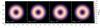Fig. 5 Gresho vortex problem advanced to t = 1.0 with preconditioned Roe fluxes for different maximum Mach numbers Mmax in the setup, as indicated in the plots. The Mach number relative to the respective Mmax is color coded.

A popular choice for a preconditioning matrix was introduced by Weiss & Smith (1995). Expressed in primitive variables, it has the form $\begin{array}{ccc}{{P}}_{{V}}\mathrm{=}\left(\begin{array}{c}\\ & & & & & \\ & & & & & \\ & & & & & \\ & & & & & \end{array}\right)\mathit{,}& & \end{array}$(36)with the parameter μ = min [ 1,max(M,M_cut) ], which should be set to the local Mach number M of the fluid (e.g., numerically defined the average of both sides of the interface). Its lower limit, M_cut, avoids singularity of P_V. To prevent the preconditioner from acting on supersonic flow, μ is limited from above to 1. At locations in the flow where M ≥ 1, the preconditioner reduces to the identity matrix, and the original Roe scheme is recovered.

For the preconditioner (36)we performed the same low-Mach analysis as in Sect. 7. This yields $\begin{array}{ccc}{{P}}_{{V}}^{-1}\left|{{P}}_{{V}}{{A}}_{{V}}\right|\mathrm{\propto }\left(\begin{array}{c}\\ & & & & & \\ & & & & & \\ & & & & & \\ & & & & & \end{array}\right)\mathit{.}& & \end{array}$Obviously, the scaling behavior of the preconditioned Roe matrix is almost perfectly consistent with the analytical scaling in Eq. (32). The only discrepancy is the fifth column in rows one and five, corresponding to an increased mass and energy flux in the low-Mach regime depending on the local change in pressure. This is particularly problematic in setups of stellar astrophysics, which almost always involve a hydrostatic stratification with a pressure gradient in the vertical direction. Terms in the flux function resulting from elements of the upwind matrix with incorrect scaling behavior make it then impossible to maintain the correct hydrostatic equilibrium.

We thus propose a new low-Mach preconditioning scheme for the Roe flux that ensures the correct scaling behavior in slow flows. This is achieved by using the preconditioning matrix $\begin{array}{ccc}{{P}}_{{V}}\mathrm{=}\left(\begin{array}{c}\\ & & & & & \\ & & & & & \\ & & & & & \\ & & & & & \\ & & \end{array}\right)\mathit{,}& & \end{array}$(37)with the parameter δ = 1 /μ − 1. As in Eq. (36), μ is the local Mach number limited by 1 and M_cut. The unpreconditioned case corresponds to δ = 0, which is automatically reached in regions with local Mach numbers of 1 or larger. Here, the scheme transitions continuously to the original Roe scheme.

With this scheme, an analysis of the low-Mach-number scaling behavior gives $\begin{array}{ccc}{{P}}_{{V}}^{-1}\left|{{P}}_{{V}}{{A}}_{{V}}\right|\mathrm{\propto }\left(\begin{array}{c}\\ & & & & & \\ & & & & & \\ & & & & & \\ & & & & & \end{array}\right)\mathit{.}& & \end{array}$This shows that the new scheme behaves consistently with the physical flux Jacobian matrix. None of the terms is overwhelmed by the numerical upwind artificial viscosity for M_r → 0, as was the case for the unpreconditioned Roe scheme and the scheme preconditioned with matrix (36).

We remark, however, that our new flux function is not unique – there may be other ways of constructing preconditioning matrices to correct the low-Mach-number scaling of the Roe flux. It is also not proved that our scheme is numerically stable. On the basis of the Gresho vortex problem and the Kelvin-Helmholtz instability (see Sect. 9), however, we demonstrate that the scheme has the desired behavior.

9. Tests of the low-Mach-number solver

9.1. Gresho vortex problem

We evolved the Gresho vortex problem from t = 0 to t = 1 with our new low-Mach-number solver, preconditioned with matrix (37). Results for maximum Mach numbers of M_max = 10^{− n}, n = 1,2,3,4 are shown in Fig. 5, but tests down to n = 10 did not detect any deviation from the illustrated behavior. As before, all these runs were performed with implicit ESDIRK34 time discretization using the advective CFL criterion (15). Because the modifications introduced in our new method are in the spatial discretization alone, we expect it to work for explicit time discretization as well as for implicit schemes. To demonstrate this, we performed some of the tests using the explicit RK3 scheme (Shu & Osher 1988). While for low Mach numbers this is computationally very inefficient compared to the implicit case, the amount of dissipation is almost identical (see Table 1). In our tests we found no time-step restriction other than the usual acoustic CFL condition that is derived from the physical signal velocities.

Our tests tests impressively demonstrate the performance of the new solver. The representation of the Gresho vortex does not degrade with lower Mach numbers, even if it is decreased by nine orders of magnitude. Visually, no differences can be found in the plots shown in Fig. 5, and this trend continues to even lower Mach numbers.

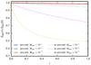Fig. 6 Temporal evolution of the total kinetic energy Ekin(t) relative to its initial value Ekin(0) in the Gresho vortex problem. For different initial Mach numbers simulations were run with (solid) and without (dotted) flux preconditioning. The lines for the preconditioned scheme show very low dissipation and are virtually indistinguishable, that is, independent of the Mach number. The final values are listed in Table 1.

This is confirmed in Fig. 6, where the evolution of the total kinetic energy is shown over one full revolution of the vortex for different setups and compared to the results obtained without preconditioning. No signs of instability of our scheme are detected, and only ≤2.3% of the initial energy is lost over the simulation time for all cases with preconditioning (see the corresponding rows of Table 1, labeled “preconditioned”). In contrast, already at a moderately low initial Mach number of 10^-1, the unpreconditioned solver loses more than 5.5% of the kinetic energy in the same setup. This shows that the numerical dissipation of the scheme is generally reduced by preconditioning.

At lower Mach numbers, the loss of kinetic energy drastically increases for the unpreconditioned method, while it is virtually unchanged for the preconditioned case. Thus, the second (and most important) observation is that the evolution of the kinetic energy is independent of the maximum Mach numbers M_max in the setup when applying our low-Mach-number preconditioner. We thus conclude that our new solver matches the design goals of a Mach-number-independent dissipation.

9.2. Kelvin-Helmholtz instability

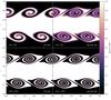Fig. 7 Advection of a passive scalar in the setup described in Sect. 9.2. The left panels were computed using the unmodified Roe scheme. In the right panels, the flux preconditioning method from Eq. (35)was used with the matrix from Eq. (37). Top panels: low-resolution simulations (1282), bottom panels: same setup at higher resolution (10242). All panels show the state at a nondimensional time of 3.0. Initially, the central (rightward-flowing) region had a value of X = 1 and the upper and lower (leftward-flowing) regions had a value of X = 0.

Although the Gresho vortex provides a useful testbed for the performance of numerical hydrodynamics solvers at low Mach numbers, its solution is essentially a steady state because of its symmetry. A true time-dependent test problem that is also closer to astrophysical application is the Kelvin-Helmholtz instability, which arises at the interface of two shearing flows. Its analytic theory was set out by Chandrasekhar (1961). There, however, the initial conditions were arranged using a sharp discontinuity. This is unsuitable for comparing different numerical discretizations and resolutions because the time and place of the initial development of instabilities entirely depend on random numerical effects. To prevent this, we instead employed the setup of McNally et al. (2012), which provides smooth initial conditions and an initial perturbation perpendicular to the interface between the shearing flows.

To solve the homogeneous Euler equations, we chose a computational domain of [ 0,1 ] × [ 0,1 ] with periodic boundaries in both directions. The problem was set up in nondimensional variables so that the Mach number could easily be adjusted. The domain was split into four regions, the leftward-moving upper (y> 0.75) and lower (y< 0.25) parts, and the rightward-moving center (0.25 <y< 0.75), which, in turn, was split into two regions to enable a smooth transition. The initial conditions were $\begin{array}{ccc}\mathit{p}& \mathrm{=}& \mathrm{2.5}\mathit{,}\\ \mathit{\varrho }& \mathrm{=}& \{\begin{array}{c}\\ & \\ & \\ & \\ & \end{array}\\ \mathit{u}& \mathrm{=}& \{\begin{array}{c}\\ & \\ & \\ & \\ & \end{array}\end{array}$We fixed the parameters to ϱ₁ = 1.0, ϱ₂ = 2.0, ϱ_m = (ϱ₁ − ϱ₂)/2, u₁ = 0.5, u₂ = −0.5, u_m = (u₁ − u₂)/2, and L = 0.025. The equation of state is that of an ideal gas with γ = 5/3.

The instability is seeded with an initial perturbation in the transverse velocity given by $\begin{array}{ccc}\mathit{v}\mathrm{=}{\mathrm{10}}^{-2}\sin \mathrm{\left(}\mathrm{2}\mathit{\pi x}\mathrm{\right)}\mathit{.}& & \end{array}$This results in a single mode being excited.

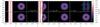Fig. 8 Logarithmic Mach number of a plane sound wave packet propagating through the Gresho vortex. The upper row shows the unpreconditioned Roe solver, the lower row was computed using the preconditioned Roe solver. The columns show the Mach number at the beginning (left), when the wave is just passing through the vortex (center left), some time after the sound wave has left the domain (center right), and after a full rotation of the vortex (right).

To adjust the Mach number of this setup to our needs, we set the reference quantities to ϱ_r = 1, p_r = 2.5, x_r = 1. The reference Mach number M_r is used as a parameter to prescribe the Mach number of the flow. The other reference quantities are then computed from this minimal set of reference quantities using ${\mathit{c}}_{\mathrm{r}}\mathrm{=}\sqrt{{\mathit{p}}_{\mathrm{r}}\mathit{/}{\mathit{\varrho }}_{\mathrm{r}}}$ and u_r = M_rc_r.

With this initial setup, we carried out simulations at Mach number 10^-2, one with the original (unpreconditioned) Roe scheme and one with flux preconditioning according to our matrix (37). For each case we performed a low-resolution run for which the domain was discretized on a numerical grid of 128² cells, and a high-resolution run with 1024² cells. A passive scalar quantity X was advected with the fluid flow for better illustration of the mixing of the layers. Its initial value is X = 1 in the center (0.25 ≤ y< 0.75) and X = 0 outside. All runs used second-order reconstruction and the implicit ESDIRK34 time-stepping scheme with an advective CFL criterion according to Eq. (15).

The results at nondimensional time 3.0 are shown in Fig. 7. As we solve the homogeneous Euler equations without any diffusion, all mixing that takes place is solely due to numerical errors. Ideally, every turnover of the instability should remain visible in the simulation because the interface is distorted, but no mixing occurs. This is clearly the case for the high-resolution runs shown in the bottom row of Fig. 7.

The high-resolution runs are very similar and differ only in the innermost part of the vortex. Here, the simulation with the unpreconditioned Roe flux shows some diffusive effects, which are absent for the preconditioned flux. In case of the low-resolution runs the difference is much more pronounced. With flux preconditioning the solution is qualitatively similar to the high-resolution runs. The unmodified Roe flux significantly smears out the flow and results in a different morphology than the other runs. This example illustrates that while the problems of standard flux functions at low Mach numbers can be partially alleviated by higher resolution, they still appear close to the grid scale. From a different perspective, one can state that use of the preconditioned flux at low resolution helps to reproduce results that would normally require much better resolution and thus more computational resources.

9.3. Gresho vortex combined with a sound wave

The previous two test problems are both tests that reside strictly in the low-Mach, nearly incompressible regime. While the preconditioned Roe scheme handles these cases well, its unique strength lies in handling of situations were compressible and incompressible conditions coexist on the same grid. To test the performance, we constructed a new problem using the Gresho vortex as a basis. The domain was extended to the left and comprised 80 × 40 grid cells. In the 40 × 40 cells on the right-hand side of the domain, the Gresho vortex was set up as described in Sect. 4 with M_max = 10^-3. In the 40 × 40 cells to the left of it, we placed a plane sound wave packet propagating to the right toward the vortex. The initial condition of the sound wave packet is given by 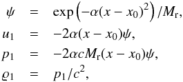$\begin{array}{ccc}\mathit{\psi }& \mathrm{=}& \exp \mathrm{(}\mathrm{-}\mathit{\alpha }\mathrm{(}\mathit{x}\mathrm{-}{\mathit{x}}_{\mathrm{0}}{\mathrm{)}}^{\mathrm{2}}\mathrm{)}\mathit{/}{\mathit{M}}_{\mathrm{r}}\mathit{,}\\ {\mathit{u}}_{\mathrm{1}}& \mathrm{=}& \mathrm{-}\mathrm{2}\mathit{\alpha }\mathrm{(}\mathit{x}\mathrm{-}{\mathit{x}}_{\mathrm{0}}\mathrm{)}\mathit{\psi ,}\\ {\mathit{p}}_{\mathrm{1}}& \mathrm{=}& \mathrm{-}\mathrm{2}\mathit{\alpha c}{\mathit{M}}_{\mathrm{r}}\mathrm{(}\mathit{x}\mathrm{-}{\mathit{x}}_{\mathrm{0}}\mathrm{)}\mathit{\psi ,}\\ {\mathit{\varrho }}_{\mathrm{1}}& \mathrm{=}& {\mathit{p}}_{\mathrm{1}}\mathit{/}{\mathit{c}}^{\mathrm{2}}\mathit{,}\end{array}$with α = (0.1)^-2 controlling the width of the packet, x₀ = −0.5 denoting the position of the center, and $\mathit{c}\mathrm{=}\sqrt{\mathit{\gamma }{\mathit{p}}_{\mathrm{0}}\mathit{/}{\mathit{\varrho }}_{\mathrm{0}}}$ the sound speed. The nondimensional values u₁, p₁, and ϱ₁ were added to the background states of the Gresho vortex problem. This resulted in a sound wave with a maximum Mach number of 10^-2.

The initial Mach numbers of this setup are shown in the left panels of Fig. 8. We expect the wave to pass through the vortex without interference as the compressible and incompressible solutions decouple in the low-Mach limit (see the discussion in Sect. 3). The top and bottom boundary conditions of the domain are periodic, as before. The left and right boundaries, however, are now chosen to ensure that the wave leaves the domain without producing numerical artifacts. This is achieved by implementing the far-field boundary condition of Ghidaglia & Pascal (2005).

We computed the time evolution of the problem using the standard Roe scheme. In a second run, the calculation was repeated, but this time we applied our new preconditioning technique to the numerical fluxes. For time stepping, we used the explicit RK3 method with the acoustic CFL criterion because we need to limit the time steps to the sound crossing time to resolve the sound wave. The Mach numbers for different times are shown in Fig. 8. The tests demonstrate that the sound wave passes through the vortex without interference in both runs, as expected. However, after one full revolution, the high dissipation in the unpreconditioned case leads to a destruction of the vortex (see upper right panel of Fig. 8). We emphasize that this is the same effect as studied before and not caused by the interaction with the sound wave that has left the domain long before. In contrast, the vortex is preserved over one full revolution if preconditioning is applied (lower right panel of Fig. 8).

The test demonstrates that our preconditioning method, while enabling to accurately represent flows at low Mach numbers, retains the capability of modeling compressible hydrodynamics phenomena on the same grid. The propagation of the sound waves in the unpreconditioned and preconditioned cases is identical (compare upper and lower panels in the second column of Fig. 8). In particular, its propagation speed is not altered by the preconditioning technique. This shows that our method is perfectly capable of providing the correct solution to problems that combine compressible and incompressible hydrodynamical flows.

10. Conclusions

Many astrophysical problems involve hydrodynamical flows at low Mach numbers M. Such slow flows are solutions of the Euler equations. Based on an analysis of their solution space in the limit M → 0, we formulated two requirements for a numerical scheme to correctly treat flows at low Mach numbers: Requirement 3 is that for M → 0 incompressible solutions should be retained, provided that the initial condition was well-prepared. Requirement 3 states that in the low-Mach-number limit the total kinetic energy should be conserved.

Following the work of Turkel (1999) and Guillard & Murrone (2004), who discussed the failure of Godunov-type solvers to correctly reproduce slow flows in numerical simulations, we argued that the reason for this problem in the case of the Roe scheme is an inconsistent scaling of the Roe matrix for M → 0. The upwind viscosity term arising from it can be seen as artificial – introduced only to stabilize the numerical scheme. It should not dominate the physical flux in the low-Mach-number limit. To achieve consistency between the scalings of the Roe matrix and the Jacobian of the physical flux, preconditioning was proposed. We introduced a new preconditioning matrix that ensures perfect consistency and demonstrated the capability of the novel scheme to reproduce flows at low Mach numbers on two examples: the Gresho vortex and the Kelvin-Helmholtz instability.

The Gresho vortex is a solution of the incompressible Euler equations, and we showed that our new scheme, in contrast to conventional unpreconditioned approaches, reproduces it satisfactorily even at very low Mach numbers. Thus, our method complies with requirement 3.

Of course, some kinetic energy is lost as a result of discretization errors. This means that requirement 3 is not fully satisfied. However, the loss of kinetic energy is substantially lower than in conventional schemes, even at moderately low Mach numbers. At very low Mach numbers the difference is even more pronounced. While the motion of the Gresho vortex is dissipated away quickly in the unpreconditioned scheme, we observed no deterioration in the quality of the solution with lower Mach number in our approach, and it therefore is applicable to almost arbitrarily slow flows. This is attributed to the preconditioning of the upwind artificial viscosity. This term dominates numerical dissipation at low Mach numbers in conventional schemes, and this undesired effect is removed in our method.

We emphasize that our preconditioning technique only affects an artificial term in the numerical flux that was introduced to stabilize the scheme. Its choice is somewhat arbitrary. Thus, compared to conventional methods, our new scheme is merely a different numerical approximation to the solution of the same set of equations. This distinguishes our technique from other approaches of numerically modeling flows at low Mach numbers. These usually start out from a modification of the system to be solved. Thus, our new method has the convenient property that well-tested standard Godunov-type solvers can be used (when properly preconditioned). In particular, we note that our modifications do not affect the equation of state and there is no restriction to an ideal gas. Well-known extensions of finite-volume schemes to general equations of state can be used, which is important for astrophysical applications. In addition, in terms of the flow regimes to be modeled, our scheme is more generally applicable. It can be used for flows at low Mach numbers, but because the underlying equations are unchanged, it also applies to the compressible regime, where preconditioning is switched off by construction.

These special properties imply that our new scheme promises to be able to successfully model hydrodynamic processes in stellar astrophysics that are inaccessible for conventional methods. A thorough description of its numerical implementation will be given in a forthcoming publication.

Acknowledgments

We thank Konstantinos Kifonidis for pointing out Turkel’s preconditioning technique to us. This inspired the development of the scheme presented here. We also gratefully acknowledge stimulating discussions with Christian Klingenberg and Markus Zenk. The work of FKR and PVFE is supported by the Deutsche Forschungsgemeinschaft (DFG) through the graduate school on “Theoretical Astrophysics and Particle Physics” (GRK 1147). F.K.R. receives additional support from the Emmy Noether Program (RO 3676/1-1) of DFG and the ARCHES prize of the German Federal Ministry of Education and Research (BMBF).

References

Appendix A: Variable transformation matrices

Here we present the Jacobian matrices for the transformation between conservative variables U, defined in Eq. (2), and primitive variables V, defined in Eq. (30). V can be expressed in terms of the components of U by $\begin{array}{ccc}{V}\mathrm{=}\left(\begin{array}{c}\\ \\ \\ \\ \end{array}\right)\mathit{,}& & \end{array}$where p(ϱ,ϵ,X) is an arbitrary equation of state, depending on mass density, internal energy per volume ϵ, and composition.

The Jacobian matrix for the transformation from U to V can then be directly calculated: $\begin{array}{ccc}\frac{\mathit{\partial }{V}}{\mathit{\partial }{U}}\mathrm{=}\left(\begin{array}{c}\\ & & & & & \\ & & & & & \\ & & & & & \\ & & & & & \end{array}\right)\mathit{,}& & \end{array}$with $\begin{array}{ccc}\mathit{\alpha }\mathrm{=}{\mathit{p}}_{\mathit{\varrho }}\mathrm{+}\frac{\mathrm{1}}{\mathrm{2}}{\mathit{M}}_{\mathrm{r}}^{\mathrm{2}}{\mathit{p}}_{\mathit{ϵ}}\mathrm{(}{\mathit{u}}^{\mathrm{2}}\mathrm{+}{\mathit{v}}^{\mathrm{2}}\mathrm{+}{\mathit{w}}^{\mathrm{2}}\mathrm{)}\mathrm{-}\frac{{\mathit{p}}_{\mathit{X}}\mathit{X}}{\mathit{\varrho }}\mathrm{·}& & \end{array}$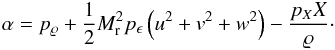This introduces abbreviations for the derivatives of the equation of state, $\begin{array}{ccc}{\mathit{p}}_{\mathit{\varrho }}\mathrm{=}{\frac{\mathit{\partial p}}{\mathit{\partial \varrho }}|}_{\mathit{ϵ,X}} {\mathit{p}}_{\mathit{ϵ}}\mathrm{=}{\frac{\mathit{\partial p}}{\mathit{\partial ϵ}}|}_{\mathit{\varrho ,X}} {\mathit{p}}_{\mathit{X}}\mathrm{=}{\frac{\mathit{\partial p}}{\mathit{\partial X}}|}_{\mathit{\varrho ,ϵ}}\mathit{.}& & \end{array}$

Inverting the above matrix yields the Jacobian for the conversion from V to U, $\begin{array}{ccc}\frac{\mathit{\partial }{U}}{\mathit{\partial }{V}}\mathrm{=}{\left(\frac{\mathit{\partial }{V}}{\mathit{\partial }{U}}\right)}^{-1}\mathrm{=}\left(\begin{array}{c}\\ & & & & & \\ & & & & & \\ & & & & & \\ & & & & & \\ & & & & & \\ & & & & & \end{array}\right)\mathit{,}& & \end{array}$with $\begin{array}{ccc}\mathit{\beta }\mathrm{=}\frac{\mathrm{1}}{\mathrm{2}}{\mathit{M}}_{\mathrm{r}}^{\mathrm{2}}\mathrm{(}{\mathit{u}}^{\mathrm{2}}\mathrm{+}{\mathit{v}}^{\mathrm{2}}\mathrm{+}{\mathit{w}}^{\mathrm{2}}\mathrm{)}\mathrm{-}\frac{{\mathit{p}}_{\mathit{\varrho }}}{{\mathit{p}}_{\mathit{ϵ}}}\mathrm{·}& & \end{array}$An advantage of this approach is that it uses the same derivatives of the equation of state. This avoids differentiating the (possibly tabulated) equation of state in its inverted form.

All Tables

All Figures

	Fig. 1 Setup of the Gresho vortex problem for Mmax = 0.1. The Mach number is color coded.
In the text

	Fig. 2 Gresho vortex problem advanced to t = 1.0 with a central flux discretization scheme for different maximum Mach numbers Mmax in the setup, as indicated in the plots. The Mach number relative to the respective Mmax is color coded.
In the text

	Fig. 3 Temporal evolution of the total kinetic energy Ekin(t) relative to its initial value Ekin(0) in the Gresho vortex problem advanced with central fluxes. The cases for Mmax = 10-1, 10-2, 10-3, and 10-4 are overplotted but are virtually indistinguishable.
In the text

	Fig. 4 Gresho vortex problem advanced to t = 1.0 with the Roe flux discretization scheme for different maximum Mach numbers Mmax in the setup, as indicated in the plots. The Mach number relative to the respective Mmax is color coded.
In the text

	Fig. 5 Gresho vortex problem advanced to t = 1.0 with preconditioned Roe fluxes for different maximum Mach numbers Mmax in the setup, as indicated in the plots. The Mach number relative to the respective Mmax is color coded.
In the text

Fig. 6 Temporal evolution of the total kinetic energy Ekin(t) relative to its initial value Ekin(0) in the Gresho vortex problem. For different initial Mach numbers simulations were run with (solid) and without (dotted) flux preconditioning. The lines for the preconditioned scheme show very low dissipation and are virtually indistinguishable, that is, independent of the Mach number. The final values are listed in Table 1.

In the text

Fig. 7 Advection of a passive scalar in the setup described in Sect. 9.2. The left panels were computed using the unmodified Roe scheme. In the right panels, the flux preconditioning method from Eq. (35)was used with the matrix from Eq. (37). Top panels: low-resolution simulations (1282), bottom panels: same setup at higher resolution (10242). All panels show the state at a nondimensional time of 3.0. Initially, the central (rightward-flowing) region had a value of X = 1 and the upper and lower (leftward-flowing) regions had a value of X = 0.

In the text

Fig. 8 Logarithmic Mach number of a plane sound wave packet propagating through the Gresho vortex. The upper row shows the unpreconditioned Roe solver, the lower row was computed using the preconditioned Roe solver. The columns show the Mach number at the beginning (left), when the wave is just passing through the vortex (center left), some time after the sound wave has left the domain (center right), and after a full rotation of the vortex (right).

In the text

References

- Almgren, A. S., Bell, J. B., & Zingale, M. 2007, J. Phys. Conf. Ser., 78, 012085 [NASA ADS] [CrossRef] [Google Scholar]
- Birken, P. 2008, Z. angewandte Math. Phys., 59, 416 [CrossRef] [Google Scholar]
- Brown, B. P., Vasil, G. M., & Zweibel, E. G. 2012, ApJ, 756, 109 [Google Scholar]
- Browning, M. K., Brun, A. S., & Toomre, J. 2004, ApJ, 601, 512 [NASA ADS] [CrossRef] [Google Scholar]
- Chandrasekhar, S. 1961, Hydrodynamic and Hydromagnetic Stability (Oxford: Clarendon Press) [Google Scholar]
- Cinnella, P. 2006, Comput. Fluids, 35, 1264 [CrossRef] [Google Scholar]
- Dellacherie, S. 2010, J. Comput. Phys., 229, 978 [Google Scholar]
- Ghidaglia, J. 2005, Eur. J. Mech. B Fluids, 24, 1 [NASA ADS] [CrossRef] [Google Scholar]
- Glatzmaier, G. A. 1984, J. Comput. Phys., 55, 461 [Google Scholar]
- Godunov, S. K. 1959, Matematicheskii Sbornik, 47, 271 [Google Scholar]
- Gresho, P. M., & Chan, S. T. 1990, Int. J. Num. Meth. Fluids, 11, 621 [Google Scholar]
- Grimm-Strele, H., Kupka, F., & Muthsam, H. J. 2014, Comput. Phys. Comm., 185, 764 [Google Scholar]
- Guillard, H., & Murrone, A. 2004, Comput. Fluids, 33, 655 [CrossRef] [Google Scholar]
- Guillard, H., & Viozat, C. 1999, Comput. Fluids, 28, 63 [CrossRef] [MathSciNet] [Google Scholar]
- Happenhofer, N., Grimm-Strele, H., Kupka, F., Löw-Baselli, B., & Muthsam, H. 2013, J. Comput. Phys., 236, 96 [NASA ADS] [CrossRef] [Google Scholar]
- Kennedy, C. A., & Carpenter, M. H. 2001, Additive Runge-Kutta Schemes for Convection-Diffusion-Reaction Equations, Tech. rep., NASA Technical Memorandum [Google Scholar]
- Kifonidis, K., & Müller, E. 2012, A&A, 544, A47 [NASA ADS] [CrossRef] [EDP Sciences] [Google Scholar]
- Kwatra, N., Su, J., Grétarsson, J. T., & Fedkiw, R. 2009, J. Comput. Phys., 228, 4146 [NASA ADS] [CrossRef] [Google Scholar]
- Landau, L. D., & Lifshitz, E. M. 1959, Course of Theoretical Physics, 6, Fluid Mechanics (Oxford: Pergamon Press) [Google Scholar]
- Liska, R., & Wendroff, B. 2003, SIAM J. Scientific Computing, 25, 995 [Google Scholar]
- Mary, I., Sagaut, P., & Deville, M. 2000, Comput. Fluids, 29, 119 [CrossRef] [Google Scholar]
- McNally, C. P., Lyra, W., & Passy, J.-C. 2012, ApJS, 201, 18 [NASA ADS] [CrossRef] [Google Scholar]
- Miesch, M. S. 2005, Liv. Rev. Sol. Phys., 2, 1 [Google Scholar]
- Miesch, M. S., Elliott, J. R., Toomre, J., et al. 2000, ApJ, 532, 593 [NASA ADS] [CrossRef] [Google Scholar]
- Mottura, L., Vigevano, L., & Zaccanti, M. 1997, J. Comput. Phys., 138, 354 [NASA ADS] [CrossRef] [Google Scholar]
- Muthsam, H. J., Kupka, F., Löw-Baselli, B., et al. 2010, New Astron., 15, 460 [NASA ADS] [CrossRef] [Google Scholar]
- Nemec, M., & Zingg, D. W. 2000, AIAA Journal, 38, 402 [NASA ADS] [CrossRef] [Google Scholar]
- Nonaka, A., Almgren, A. S., Bell, J. B., et al. 2010, ApJS, 188, 358 [NASA ADS] [CrossRef] [Google Scholar]
- Renze, P., Schröder, W., & Meinke, M. 2008, Int. J. Heat and Fluid Flow, 29, 18 [CrossRef] [Google Scholar]
- Roe, P. 1981, J. Comput. Phys., 43, 357 [Google Scholar]
- Schochet, S. 1994, J. Differential Equations, 114, 476 [Google Scholar]
- Shu, C.-W., & Osher, S. 1988, J. Comput. Phys., 77, 439 [Google Scholar]
- Sutherland, B. 2010, Internal Gravity Waves (Cambridge University Press) [Google Scholar]
- Talon, S., Vincent, A., Michaud, G., & Richer, J. 2003, J. Comput. Phys., 184, 244 [Google Scholar]
- Toro, E. F. 2009, Riemann Solvers and Numerical Methods for Fluid Dynamics: A Practical Introduction (Springer) [Google Scholar]
- Turkel, E. 1999, Ann. Rev. Fluid Mech., 31, 385 [NASA ADS] [CrossRef] [Google Scholar]
- Turkel, E., Fiterman, A., & Van Leer, B. 1993, Preconditioning and the limit to the incompressible flow equations, ICASE Report 93-42, Institute for Computer Applications in Science and Engineering, NASA Langley Research Center [Google Scholar]
- van Leer, B. 1979, J. Comput. Phys., 32, 101 [Google Scholar]
- Viallet, M., Baraffe, I., & Walder, R. 2011, A&A, 531, A86 [NASA ADS] [CrossRef] [EDP Sciences] [Google Scholar]
- Viallet, M., Baraffe, I., & Walder, R. 2013, A&A, 555, A81 [NASA ADS] [CrossRef] [EDP Sciences] [Google Scholar]
- Vinokur, M., & Montagné, J.-L. 1990, J. Comput. Phys., 89, 276 [NASA ADS] [CrossRef] [Google Scholar]
- Volpe, G. 1993, AIAA Journal, 31, 49 [NASA ADS] [CrossRef] [Google Scholar]
- Weiss, J. M., & Smith, W. A. 1995, AIAA Journal, 33, 2050 [NASA ADS] [CrossRef] [Google Scholar]