| Issue |
A&A
Volume 576, April 2015
|
|
|---|---|---|
| Article Number | A7 | |
| Number of page(s) | 16 | |
| Section | Numerical methods and codes | |
| DOI | https://doi.org/10.1051/0004-6361/201424602 | |
| Published online | 13 March 2015 | |
MORESANE: MOdel REconstruction by Synthesis-ANalysis Estimators
A sparse deconvolution algorithm for radio interferometric imaging
1
Laboratoire Lagrange, UMR 7293, Université Nice Sophia-Antipolis, CNRS,
Observatoire de la Côte d’Azur,
06300
Nice,
France
e-mail:
This email address is being protected from spambots. You need JavaScript enabled to view it.
2
Centre for Radio Astronomy Techniques & Technologies
(RATT), Department of Physics and Electronics, Rhodes University,
PO Box 94, 6140
Grahamstown, South
Africa
3
SKA South Africa, 3rd Floor, The Park, Park Road,
7405
Pinelands, South
Africa
Received: 15 July 2014
Accepted: 13 December 2014
Abstract
Context. Recent years have been seeing huge developments of radio telescopes and a tremendous increase in their capabilities (sensitivity, angular and spectral resolution, field of view, etc.). Such systems make designing more sophisticated techniques mandatory not only for transporting, storing, and processing this new generation of radio interferometric data, but also for restoring the astrophysical information contained in such data.
Aims.In this paper we present a new radio deconvolution algorithm named MORESANEand its application to fully realistic simulated data of MeerKAT, one of the SKA precursors. This method has been designed for the difficult case of restoring diffuse astronomical sources that are faint in brightness, complex in morphology, and possibly buried in the dirty beam’s side lobes of bright radio sources in the field.
Methods.MORESANE is a greedy algorithm that combines complementary types of sparse recovery methods in order to reconstruct the most appropriate sky model from observed radio visibilities. A synthesis approach is used for reconstructing images, in which the synthesis atoms representing the unknown sources are learned using analysis priors. We applied this new deconvolution method to fully realistic simulations of the radio observations of a galaxy cluster and of an HII region in M 31.
Results.We show that MORESANE is able to efficiently reconstruct images composed of a wide variety of sources (compact point-like objects, extended tailed radio galaxies, low-surface brightness emission) from radio interferometric data. Comparisons with the state of the art algorithms indicate that MORESANE provides competitive results in terms of both the total flux/surface brightness conservation and fidelity of the reconstructed model. MORESANE seems particularly well suited to recovering diffuse and extended sources, as well as bright and compact radio sources known to be hosted in galaxy clusters.
Key words: methods: numerical / methods: data analysis / techniques: image processing / techniques: interferometric
© ESO, 2015
1. Introduction
In the past 40 years, the radio community has mainly been using, as a reliable and well-understood method for deconvolving interferometric data, the CLEAN algorithm and its different (including multiresolution) variants e.g., 32; 62; 14. Even if other methods have been designed during this period see for instance 35; 47; 53; 29 none has become as popular and as widely used as CLEAN in practice.
Deep and/or all-sky radio surveys characterized by sub-mJy sensitivity and arcsec angular resolution, as well as by high (>1000) signal-to-noise and wide spatial dynamic ranges (challenging features for a proper deconvolution and reconstruction of both bright and diffuse radio components) will be available in the next decades thanks to incoming and future radio facilities, such as the Low Frequency Array (LOFAR), the Australian Square Kilometre Array Pathfinder (ASKAP, Australia), and the Karoo Array Telescope (MeerKAT, South Africa). These revolutionary radio telescopes, operating in a wide region of the electromagnetic spectrum (from 10 MHz to 15 GHz), are the technical and scientific pathfinders of the Square Kilometre Array (SKA). With a total collecting area of one square kilometer, SKA will be the largest telescope ever built1.
Recently, much attention has been paid in various fields of the signal- and image-processing community to the theory of compressed sensing CS, 18; 9. Although the current theoretical results of CS do not provide means of reconstructing realistic radio interferometric images more accurately, there is one key domain that allows doing so, and the applied CS literature often builds on this domain: sparse representations. Sparse approximation through dedicated representations is a theory per se, and it has a very long history 36. In the signal processing community and, in particular, in denoising and compression, sparsity principles opened a new era when Donoho and Johnstone 20 proved the minimax optimality of thresholding rules in wavelet representation spaces. We propose in Sect. 3 a survey of the use of sparse representations in radio interferometry.
In this paper we describe a new deconvolution algorithm named MORESANE (MOdel REconstruction by Synthesis-ANalysis Estimators), which combines complementary types of sparse representation priors. MORESANE has been designed to restore faint diffuse astronomical sources, with a particular interest in recovering the diffuse intracluster radio emission from galaxy clusters. These structures are known to host a variety of radio sources: compact and bright radio galaxies, which can present a tailed morphology modeled by the interaction with the intracluster medium ICM; e.g., 23; radio bubbles filling holes in the ICM distribution and rising buoyantly through the thermal gas observed in X-rays e.g., 17; Mpc-scale, very low surface-brightness sources of radio emission, which are related to the presence of relativistic electrons (Lorentz factors γ ≫ 1000) and weak magnetic fields (~μGauss) in the ICM e.g., 25.
An increased capability of detecting diffuse radio emission is, of course, very relevant not only for galaxy cluster studies, but also for other astronomical research areas, such as supernova remnants e.g., 5, radio continuum emission from the Milky Way e.g., 2, star-forming regions in nearby galaxies e.g., 46, and possibly, in the near future, filaments of diffuse radio emission related to electron acceleration in the cosmic web (Vazza et al., in prep.).
After an introduction to the radio interferometric model and sparse representations, in Sects. 2 and 3 respectively, we justify and describe our new algorithm in Sects. 4 and 5, respectively. Applications of MORESANE to both simplified and fully realistic simulations of test images are presented in Sect. 6. We conclude with a discussion of our results and list several evolutions for MORESANE (Sect. 7).
A word on the notations before starting. We denote matrices by bold upper case letters (e.g., M), vectors either by bold lower case letters (e.g., v) or by indexed matrix symbols when they correspond to a column of a matrix (e.g., Mi is the ith column of M). Scalars (and complex numbers) are not in boldface except if they correspond to components of a vector (e.g., vi is the ith component of v) or of a matrix (e.g., Mij is the component at the ith row and jth column of M).
2. Radio interferometric imaging
Radio interferometric data are obtained from the response of the radio interferometer to the electric field coming from astrophysical sources. The electro-magnetic radiation emitted by all the observed celestial sources will arrive at an observation point r, producing a total received electric field (Eν(r)) that we consider as a scalar and quasi monochromatic quantity. For the sake of simplicity, we omit the index ν in the following.
For an interferometer, each radio measurement, called complex visibility, corresponds to the spatial coherence of the electric field measured by a pair of antennas that have coordinates r1 and r259:  (1)where ⟨·⟩ represents time averaging and ∗ the complex conjugate.
The spatial coherence function of the electric field E depends only on the baseline vector r1 − r2, and it is correlated to the intensity distribution of incoming radiation I(s) (where s is the unit vector denoting the direction on the sky) through  (2)In the equation above, ⊤ stands for transpose, c is the speed of light, dΩ the differential solid angle, and we assume an isotropic antenna response. Since interferometer antennas have a finite size, an additional factor can enter into (2). This is the primary beam pattern, which describes the sensitivity of the interferometer elements as a function of direction s.
In the previous equation, the baseline vector b = r1 − r2 can be expressed with components measured in units of wavelength (u,v,w), where w points in the direction of the line of sight and (u,v) lie on its perpendicular plane. The direction cosines (l,m,n) define the position of a distant source on the celestial sphere, with (l,m) measured with respect to (u,v) axis. In the adopted formalism, l2 + m2 + n2 = 1, so the coordinates
(l,m) are sufficient to specify a given point in the celestial sphere. Using this formalism; (2)can be written as
 (3)In the particular cases where all measurements are acquired in a plane (i.e. w = 0, such as with east-west interferometers) and/or the sources are limited to a small region of the sky (i.e. n ≃ 1, for small fields of view, which is the case considered in this paper); (3)reduces to a two-dimensional Fourier transform.
In the impossible case of visibilities measured on the whole (u,v) plane, inverse Fourier transform of V(u,v) would thus directly yield the sky brightness image I(l,m). In practice, visibilities are measured at particular points of the Fourier domain, defining the (u,v) coverage of the observations. The set of samples depends on the configuration and number of the antennas, the time grid of measurements, and the number of channels, because the baselines change with the Earth’s rotation. A sampling function M(u,v) is thus introduced, which is composed of Dirac delta function where visibilities are acquired.
After the necessary calibration step on the visibilities not described here; see, e.g., 26, the measured visibilities can be written as
 (4)where ϵ corresponds to a white Gaussian noise coming essentially from the sky, receivers, and ground pick up. In addition, a weighted sampling function can be applied to the data, with different weights assigned to different observed visibilities, depending on their reliability, their (u,v) locus (tapering function), or their density in the (u,v) plane (density weighting function) 6.
The image formed by taking the inverse Fourier transform of Vmes is called a dirty image, which is defined as the convolution of the true sky surface brightness distribution I(l,m) with the Fourier inverse transform of the sampling function M(u,v) (known as the dirty beam or the point spread function (PSF) of the array). In practice, fast Fourier transforms (FFT) are used where observed visibilities must be interpolated on a regular grid of 2N × 2M points, generating an N × M pixel image with a pixel size taken to be smaller (~1/3−1/5) than the angular resolution of the instrument. Different ways can be adopted to optimize the FFT interpolation 6, whose discussion goes beyond the purpose of this paper.
In this framework, the model for the visibility measurements can be written in matrix form as 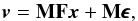 (5)where v ∈ RN is a column vector that contains the measured visibilities for the sampled frequencies and zeroes otherwise; M is a diagonal matrix with 0 and 1 on the diagonal, which expresses the incomplete sampling of the spatial frequencies; F (resp. F†) corresponds to the Fourier (resp. Fourier inverse) transform, and the vector x ∈ RN is the sky brightness image. Equivalently, the dirty image y is obtained by inverse Fourier transform of the sparse visibility map:
 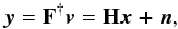 (6)where H = F†MF,H ∈ RN × RN is the convolution operator corresponding to the array’s PSF and n ∈ RN is the noise in the image domain. In this setting H is a circulant matrix operator, where every column is a shifted version of the PSF for every pixel position.
Finally, in Model (6), the noise is additive Gaussian and correlated because of the missing points in the (u,v) domain 59.
We hereafter restrict ourselves to the simplified acquisition model described above. As we shall see, accurate image deconvolution is already challenging in this case, especially for astrophysical scenes containing faint diffuse sources, along with brighter and more compact ones.
3. Sparse representations in radio interferometry
3.1. CLEAN
Radio interferometry has a long acquaintance with sparse representations. Högbom’s CLEAN algorithm 32 and the family of related methods 62; 51; 15; 49 implement ideas similar to matching pursuit 27; 37 and to ℓ1 penalization 50. In fact, in the radioastronomical community CLEAN refers to a family of algorithms (Clark’s CLEAN, Cotton-Schwab CLEAN, MultiResolution CLEAN, etc.).
A remarkable fact is that the CLEAN method remains a reference and a very well known tool for almost all radio astronomers. There may be several reasons for this. First, CLEAN is a competitive algorithm, with best results on point-like sources and less accurate recovery of extended sources. In CLEAN, the CLEAN factor does a lot: following Högbom’s original version of the algorithm, the point source’s contribution, which is the one most correlated to the data, is only partly subtracted from the data (in contrast to matching pursuit, which makes the residual orthogonal to this atom). This has the effect of creating detections at many locations and of mitigating the influence of the brightest sources. These numerous localized spikes mimic extended flux components and somewhat compensate for the point-like synthesis of the restored image once the detection is reconvolved by the clean beam. Besides, after the stopping criterion is met, the residual is added to the restored image, with the same compensating effect.
From a practical viewpoint, CLEAN is easy to implement and does not require any optimization knowledge. It is also easy to build modular versions of CLEAN with deconvolution by patches, for instance, allowing direction-dependent effects to be accounted for and image restoration and calibration processes to be coupled 58.
Finally, the greedy structure of CLEAN was probably a major advantage for devising an operational spatio-spectral radio deconvolution algorithm (to our knowledge the only algorithm allowing visibility data cubes to be deconvolved), the multiscale-multifrequency CLEAN implemented in LOFAR data processing 60. As a matter of fact, CLEAN algorithms are implemented in many standard radio-imaging softwares.
3.2. Recent works: sparse representations
In the second half of the 2000s, stellar interferometry was identified as a typical instance of compressed sensing CS, 9; 18 acquisition. Since the theoretical results of CS had shed new mathematical light on the random Fourier sampling of sparse spikes, radio interferometry has appeared as a natural case of CS, and major achievements were foreseen in this domain from CS theory. Looking back at the literature from this period to now, it seems that innovation in recent radio interferometric reconstruction methods has grown less from CS theorems (because their assumptions are most often not satisfied in practical situations) than from an unchained research activity in sparse representations and convex optimization 45. Although these domains existed long before CS, they certainly benefited from the CS success. A survey of the evolution of sparse models in the recent literature of radio interferometric image reconstruction is proposed below. These models fall into two categories, sparse analysis or sparse synthesis, a vocabulary that stems from frame theory and was studied in the context of sparse representations by Elad et al. .
3.3. Sparse synthesis
This approach assumes that the image to be restored, x, can be sparsely synthesized by a few elementary features called atoms. More precisely, x is assumed to be a linear combination of a few columns of some full rank ℓ2- normalized dictionary S, of size (N,L), with L usually greater than N:  (7)With (7), model (5)becomes
  (8)The simplest and most intuitive sparsity measure is the number of non-zero entries of x (i.e., the ℓ0 pseudo-norm), but ℓ0 is not convex. To benefit from the properties of convex optimization, the ℓ0 penalization is often relaxed and replaced by ℓ12, which still promotes strict sparsity and thus acts as a variable selection procedure (
 with 0 <p< 1 also, but leads to more difficult -non convex- optimization problems;
  does not).
In a sparsity-regularized reconstruction approach, a typical regularization term corresponding to such penalties (but there are many others) has the form  , with a regularization parameter μp ∈ R+ and it is added to the data fidelity term (the squared Euclidean norm of the error for i.i.d. Gaussian noise). The vectors γ
that will minimize the cost function:
, with a regularization parameter μp ∈ R+ and it is added to the data fidelity term (the squared Euclidean norm of the error for i.i.d. Gaussian noise). The vectors γ
that will minimize the cost function: 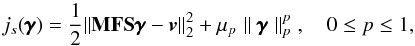 (9)will then tend to be sparse for sufficiently high values of μp. Synthesis-based approaches thus lead to solutions of the form3
 (10)The minimization problem corresponding to the particular case p = 1 is called basis pursuit denoising (BPDB) in optimization 13.
3.4. Sparse analysis
In this approach, regularity conditions on x are imposed by an operator A⊤. The sparse analysis approach consists in finding a solution x that is not correlated to some atoms (columns) of a dictionary A of size (N,L). The sparse analysis model therefore assumes that A⊤x is sparse.
Adopting a regularization term that imposes this sparsity constraint, sparse analysis approaches usually seek solutions of the form  (11)
(11)
3.5. Representations and dictionaries
The sparsity expressed through S on γ or on A⊤x requires that the signal is characterized by low dimensional subspaces. They can be orthonormal transforms (corresponding to orthonormal bases) or more generally redundant (overcomplete) dictionaries. These subspaces correspond to mathematical representations of the signal: the columns of S correspond to geometrical features that are likely to describe the unknown signal or image, while the columns of A impose geometrical constraints (in analysis).
A wide variety of such representations has been elaborated in the image-processing literature, such as canonical basis (corresponding to point-like structures), discrete cosine transform (DCT, 2D plane waves), wavelets (localized patterns in time and frequency), isotropic undecimated wavelets 52, curvelets elongated and curved patterns 54, ridgelets 8, shapelets 48, and others see 36; 56, for details on these representations and their applications..
The choice of a dictionary is made with respect to a class of images. In astronomy, wavelet dictionaries are widely used; however they are known not to be appropriate for the representation of anisotropic structures. In such cases, other transforms have been designed to capture main features of specific classes of objects. Among them, curvelets sparsify well-curved, elongated patterns (such as planetary rings or thin galaxy arms), while shapelets sparsify, for instance, various galaxy morphologies well. All of them have shown empirical efficiency and can be used in the dictionary.
To accurately model complex images with various features, one possibility is indeed to concatenate several dictionaries into a larger dictionary. However, the efficiency of a dictionary also critically depends on its size and on the existence of fast operators, without which restoration algorithms (that are iterative) cannot converge in a reasonable time. Concatenation or unions of representation spaces are now classically used in denoising and inverse problems because they can account for more complex morphological features better than standard transforms used separately an approach advocated early in Mallat & Zhang ; and Chen et al. ; see also 19; 31; 56. Such unions may allow maintaining a reasonable computational cost if fast transforms are associated to each representation space. They also provide a natural feature separation through the decomposition coefficients associated to each subdictionary. This property is indeed interesting for astronomy, where a celestial scene may contain features as different as point-like sources, rings, spirals, or smooth and diffuse components, with various spatial extensions.
3.6. Synthesis versus analysis
Analysis and synthesis priors lead to different solutions (and algorithms) for redundant dictionaries. When A and S are square and invertible, as for orthonormal bases, a change of variables with S-1 = A⊤ shows that the approaches in (10)and (11)are equivalent. A seminal study is proposed in Elad et al. , whose first result shows that when S is taken as (the pseudo-inverse of A⊤), the analysis model is restricted to a space with a lower dimension than the synthesis one. More generally, Theorem 4 of the same paper shows by more involved means that, for p = 1 and L ≥ N, a dictionary S(A⊤) exists for any ℓ1 MAP-analysis problem with full-rank analyzing operator A⊤ describing an equivalent ℓ1 MAP-synthesis problem. The converse is not true. In this sense, sparse synthesis is more general than analysis and in theory it allows better reconstruction results.
The question of how the two approaches compare in practice for usual transforms remains open, however, even for the case p = 1. The works of Carlavan et al. propose an interesting numerical comparison of the two approaches for various transforms and dictionaries in the framework of noisy deconvolution. Their conclusion is that synthesis approaches seem to be preferable at lower noise levels, while analysis is more robust at higher noise regimes.
Arias-Castro et al. report numerical experiments with redundant dictionaries showing empirically that ℓ1-synthesis may perform as well as ℓ1-analysis, while other papers highlight better results for analysis models 11. A clear and well-identified issue with synthesis is that the number of unknown (synthesis coefficients) may rapidly become prohibitive for large dictionaries, while in analysis the number of unknowns remains constant (as it corresponds to the number of image parameters in x). On the other hand, sticking to a synthesis approach with dictionaries without enough atoms may lead to rough and schematic reconstructed sources. Obtaining more theoretical and general results on the analysis vs synthesis comparison is a very interesting, active, and growing subject of research4.
In radio interferometry, each recent reconstruction algorithm has its own sparse representation model. Explicit sparse priors were indeed first expressed in the direct image space, which is typically appropriate for (but limited to) fields of unresolved stars 39; 40. In this case, the restored image can be obtained by solving the BPDN problem associated to (10)with S = I (or to (11)with A = I). This is also the approach of Wenger et al. .
To efficiently recover more complex images, sparse synthesis models involving a dictionary S taken as union of bases with a union of canonical, DCT, and orthogonal wavelets bases were proposed in Mary , Vannier et al. and Mary et al. . The restored image is in this case obtained by solving (10) with p = 1. The Compressed Sensing imaging technique BP+ of Wiaux et al. ; solves a synthesis problem (10)with p = 1 subject to an image positivity constraint, and S is a redundant dictionary of wavelets.
In Li et al. , the Compressed Sensing-based deconvolution uses the isotropic undecimated wavelet transform IUWT, 56 for S and solves (10)under a positivity constraint. We show results of this method in the simulations. The works of McEwen & Wiaux consider an analysis-based prior (total variation), for which A⊤ implements the ℓ1 norm of the discrete image gradient:  (12)where ϵ is a prescribed fidelity threshold.
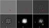 |
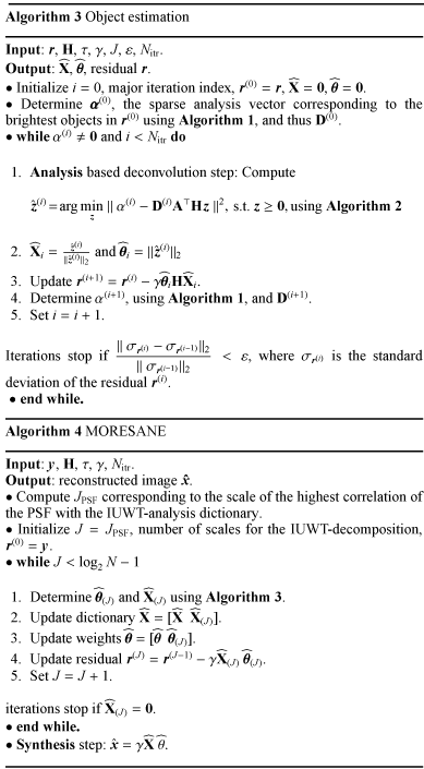
Fig. 1 Bottom right: a galaxy cluster model image, with a galaxy circled in yellow. From top left to bottom middle: IUWT analysis coefficients |


Recently, the sparsity-averaging reweighted analysis (SARA) 11 focused on an analysis criterion with a solution of the form (11)with p = 1, a positivity constraint on x and a union of wavelet bases for A. The work of Carrillo et al. presents large scale optimization strategies dedicated to this approach. Clearly, sparse models allied to optimization techniques have attracted a lot of attention in this field during the past seven or eight years.
4. Motivation for an analysis-by-synthesis approach
The imaging system described in Sect. 2 describes a linear filter whose transfer function is described by the diagonal of M. In Fourier space, this transfer function has many zeros, making the problem of reconstructing x from y underdetermined and ill-posed. In image space, the PSF has typically numerous and slowly decreasing sidelobes owing to the sparse sampling performed by the interferometer. The PSF extension and irregularity make the recovery of faint objects particularly difficult when surrounding sources that are orders of magnitude brighter.
The specific problem of restoring faint extended sources submerged by the contribution of the sidelobes of brighter and more compact sources has led us to explore a fast restoration method in Dabbech et al. , which exploits positivity and sparse priors in a hybrid manner and where MORESANE is an elaborated version. Several essential changes have been introduced in MORESANE with respect to the prototype algorithm by Dabbech et al. in order to be able to apply it on realistic radio interferometric data. The main developments include:
-
identification of the brightest object, which is now done by taking the PSF behavior into account in the wavelet domain;
-
introduction of parameters τ and γ to improve rapidity and obtain a more accurate estimation of the sky image;
-
use of the conjugate gradient instead of the projected Landweber algorithm for rapidity;
-
deconvolution scale by scale, which does not oblige the user to specify the number of scales in the IUWT.
Comprehensive surveys of the vast literature in image reconstruction methods for radio interferometric data can be found in Starck et al. (including methods from model fitting to non parametric deconvolution) and in Giovannelli & Coulais , who emphasize the particular problem of reconstructing complex (both extended and compact) sources. On this specific topic, very few other works can be found. In Magain et al. and Pirzkal et al. , the point-like sources are written in a parametric manner based on amplitudes and peak positions. Extended morphologies are accounted for in Magain et al. using a Tikhonov regularization and in Pirzkal et al. by introducing a Gaussian correlation. In Giovannelli & Coulais , a global criterion is minimized (subject to a positivity constraint), where the penalization term is the sum of the ℓ1 norm of the point-like component and the ℓ2 norm of the gradient of the extended component.
Radio interferometric image reconstruction is a research field where synthesis and analysis-sparse representations have been extensively and, in fact, almost exclusively investigated in the last few years. To be efficient on recovering faint, extended, and irregular sources in scenes with a high dynamic range, the approach we propose is hybrid in its sparsity priors and builds somewhat on ideas of Högbom and Donoho et al. . We use a synthesis approach to reconstructing the image, but we do not assume that synthesis atoms describing the sources are fixed in advance, in order to allow more flexibility in the source modeling. The synthesis dictionary atoms are learned iteratively using analysis-based priors. This iterative approach is greedy in nature and thus does not rely on global optimization procedures (such as l1 analysis or synthesis minimization) of any kind. The iterative process is important for coping with high dynamic scenes. The analysis approach allows a fast reconstruction.
5. Model reconstruction by synthesis-analysis estimators
We model the reference scene x as the superposition of P objects:  (13)where Xt, columns of X, are ℓ2-normalized objects composing x. An object may be a single source or a set of sources sharing similar characteristics in terms of spatial extension and brightness. The matrix X is an unknown synthesis dictionary of size (N,P), P ≪ N, and θ is a vector of amplitudes of size P with entries θt. The radio interferometric model (6)becomes
  (14)This model is synthesis-sparse, since the image x is reconstructed from few objects (atoms) Xt. In the proposed approach, however, the synthesis dictionary X and the amplitudes θ are learned jointly and iteratively through analysis-based priors using redundant wavelet dictionaries. Because bright sources may create artifacts spreading all over the dirty image, objects θθθtXt with the highest intensities are estimated at first, hopefully enabling the recovery of the faintest ones at last.
5.1. Isotropic undecimated wavelet transform
In the proposed method, each atom from the synthesis dictionary X will be estimated from its projection (analysis coefficients) in a suitable data representation. One possible choice for this representation, which will be illustrated below, is the isotropic undecimated wavelet transform (IUWT) 55. IUWT dictionaries have proven to be efficient in astronomical imaging because they allow an accurate modeling through geometrical isotropy and translation invariance. They also possess an associated fast transform.
We now recall some principles related to IUWT because they are important for understanding the proposed algorithm. Analyzing an image y of size N with the IUWT produces analysis coefficients that we denote ααα = A⊤y. Those are composed of J + 1 sets of wavelet coefficients, where each set is the same size as the image (see Fig. 1) and J ≤ log 2N − 1 is an integer representing the number of scales of the image decomposition. Formally α can be written as
![Mathematical equation: \hbox{${\pmb \alpha} = [{\bf w}^\top_{(1)},\hdots,{\bf w}^\top_{(J)},{\vec{a}}^\top_{(J)}]^\top$}](/articles/aa/full_html/2015/04/aa24602-14/aa24602-14-eq124.png) , where the
, where the  are wavelet coefficients (for which j = 1 represents the highest frequencies), and a(J) is a set of smooth coefficients. Important is that the data y can be recovered by y = Sααα, where S is the IUWT-synthesis dictionary corresponding to A.
An interesting feature of the IUWT is that astrophysical sources yield very specific signatures in its analysis coefficients. As an illustration, Fig. 1 highlights a galaxy in the original image of a model galaxy cluster (see below for a more detailed description) with the analysis coefficients generated by this galaxy (inside the red circles). The fingerprint let by this object is clearly visible in the first three scales. This suggests that each source can in principle be associated to a set of a few coefficients (w.r.t. the number of pixels N), which capture the source signature at its natural scales. Conversely, we may try to reconstruct the sources from the sparse set of corresponding analysis coefficients.
This is the strategy followed below, and it actually requires two steps. First, obviously, the image that we must consider for identifying the sources is the dirty image, which is noisy. This means that all analysis coefficients α are not genuinely related to astrophysical information, and some of them should be discarded as noise. Using standard procedures see, e.g., 57, the noise level can be estimated scale by scale from the wavelet coefficients using a robust median absolute deviation (MAD) 33, for instance. The resulting significant analysis coefficients, which we denote by
 , are obtained from the analysis coefficients α scale by scale, by leaving the coefficients larger than the significance threshold untouched and setting the others to 0.
Second, we need a procedure that will estimate which fraction of the significant analysis coefficients
 characterizes the brightest source(s) (because we want to remove them to see what is hidden in the background). We call this step object identification and describe it below. We will then be in a position to present the global reconstruction algorithm.
5.2. Object identification
The brightest object in the dirty image is defined from a signature defined by a subset of significant coefficients
, which we denote by αmax. The starting point for obtaining the brightest object is to locate the most significant analysis coefficient. The IUWT analysis operation A⊤y = A⊤Hx may be seen as the scalar product between the atoms
 and Hx, or equivalently of
  with x. We denote the pixel of maximal correlation score between x and one of the convolved dictionary atoms by
 ![Mathematical equation: \begin{equation} \label{bright} {k^{{\rm max}}}={\displaystyle\rm arg}\max_{{k\in [1,(N+1)\times J]}}\frac{{\bf{A}}_k^\top {{\bf H}{\vec x}}}{\Vert {\bf{A}}_k^\top {\bf H} \Vert_2 }={\displaystyle\rm arg}\max_{{k\in [1,(N+1)\times J]}}\frac{\tilde{\pmb\alpha}_k}{\Vert {\bf{A}}_k^\top {\bf H} \Vert_2 }\cdot \end{equation}](/articles/aa/full_html/2015/04/aa24602-14/aa24602-14-eq138.png) (15)This normalization ensures that if x was pure noise, kmax would pick up all atoms with the same probability. The third part of the equation is indeed valid only if
(15)This normalization ensures that if x was pure noise, kmax would pick up all atoms with the same probability. The third part of the equation is indeed valid only if  contains nonzero coefficients. We also let αmax be the wavelet coefficient at the pixel position kmax defined by (15)and jmax be the corresponding scale.
To formalize the object identification strategy, we now need two definitions from multiscale analysis 57. First, a set of spatially-connected nonzero analysis coefficients at the same dyadic scale j is called a structure and is denoted by s. (This vector is thus a set of contiguous analysis coefficients.) Typically, the red circles of Fig. 1 encircle instances of structures. Second, an object will be characterized by a set of structures leaving at different scales and connected from scale to scale. Typically, the structure in the red circles of Fig. 1 would be connected from scales j = 3 to scale j = 1 because they are vertically aligned. (More precisely, the position of the maximum wavelet coefficient of the structure at the scale j − 1 also belongs to a structure at the scale j.) In the case of Fig. 1, the structures associated to this object correspond to only one source − the circled galaxy in Fig. 1.
To estimate the whole fingerprint of the brightest object (say, the circled galaxy), we proceed as follows. First, we identify kmax and the structure smax, on scale jmax, to which the pixel position kmax belongs. The other structures of this object are searched only at lower scales (j = 1,...,jmax − 1), where its finest details live significantly. The resulting set of connected structures constitutes the significant coefficients identifying the signature of the brightest object in the data. These coefficients are stored in a sparse vector
 of dimension N × (J + 1).
Of course, instead of detecting and using only the most significant coefficient kmax in
, it can be more efficient to select a fraction of the largest coefficients on the scale jmax see, e.g., 21. In this case, the algorithm simultaneously captures structures corresponding to other sources that have intensities and natural scales that are similar to the brightest object defined only by kmax and its associated structures. In our algorithm, structures on the scale jmax are allowed to have their maximum wavelet coefficient as low as τ × αmax, where τ is a tuning parameter, which needs to be selected.The joint estimation of these objects reduces deconvolution artifacts significantly since their sidelobes in the data are taken into account simultaneously. The choice of τ within a wide range (e.g., [ 0.6 0.9 ]) does not affect the final results significantly. Only low values of τ (say 0.1) can lead to convergence problems because the fainter objects are dominated by the brighter ones.In this case,
 will capture the signature of several sources in the dirty image. The detailed description of the resulting object-identification strategy is given by Algorithm 1.
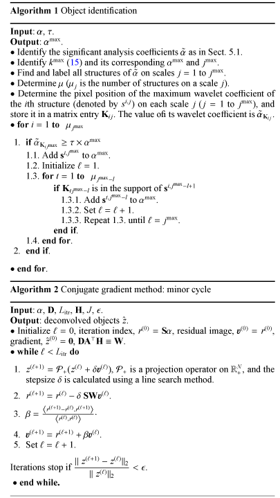
In this algorithm, the significant analysis coefficients  are found as in Sect. 5.1, as well as the maximally significant coefficients αmax, its position kmax and scale jmax (Steps 1 and 2). In Step 3, we find and label all structures on scales smaller than or equal to jmax, and we collect their number
  per scale j in μμμ = [ μμμ1..μμμjmax ]. In Step 5 we store the position of the maximum wavelet coefficient of the ith structure of scale j in the entry Kij of a matrix K. The value of this coefficient is then
  . Step 6 involves a recursive loop. Its purpose is to look for each significant structure si,jmax on scale jmax, whether there is a structure on scale jmax − 1, whose maximum is vertically aligned with it. Such a structure is included in . The process is repeated for this structure on the lower scale. This process creates a tree of significant structures that describes the object’s signature.
Once the signature of a bright object has been obtained, the object is deconvolved using  by solving approximately the following problem:
  (16)where D maps the analysis coefficients to the nonzero values of and z ≥ 0 means that all components of z are non-negative, and D is formally a diagonal matrix of size (N × (J + 1),N × (J + 1)) defined by Dkk = 1 if
  and 0 otherwise.
5.3. The MORESANE algorithm
These ideas lead to the following iterative procedure. At each iteration i, we identify a sparse vector  , using Algorithm 1, which contains the signature of the brightest object in the residual image within a range controlled by τ. The flux distribution of this object (that may correspond to several sources belonging to the same class in term of flux and angular scales) is estimated at each iteration i as one object z(i) using the extended conjugate gradient Biemond et al. as described in Algorithm 2. In the conjugate gradient, since the conjugate vector and the estimate are no longer orthogonal due to the nonlinear projection on the positive orthant, a line search method must be deployed to estimate the stepsize δ. The estimated synthesis atom corresponding to z(i) is simply
  and
and
 . The influence of this object can be removed from the residual image by subtracting
  . However, the complete removal of the bright sources contribution at each iteration could create artifacts in the residual image. Those are caused by an overestimation of the bright contributions, which in turn can impede the recovery of the faint objects. This fact is reminiscent of issues regarding proper scaling of the stepsize in descent algorithms and of CLEAN loop factor 32. To provide a less aggressive and more progressive attenuation of the bright sources’ contribution, we have introduced a loop gain γ in MORESANE as in CLEAN. Values of γ that are close to 1 lead to instability in the convergence. On the other hand, values that are too low lead to very slow convergence. We found that γ ∈ [ 0.1 0.2 ] is a good compromise. The version with γ is presented in Algorithm 3. The formal number of objects may become significantly large when using γ.
In the reconstruction of specific examples (see the next section), it appears that when large features are deconvolved at first, they somewhat capture the contribution of smaller sources, which are then not accurately restored during the subsequent iterations on small sales (they incur significant artifacts, in particular on the border of the sources). Therefore, we have opted for a general strategy (described in Algorithm 4) where Algorithm 3 is run iteratively for J = JPSF up to log 2N − 1, where J = JPSF is the scale corresponding to the highest correlation of the PSF with the analysis dictionary AT. As the considered number of scales become larger, we also include all smaller scales in the dictionary, because small structures may become significant once the contributions of other sources have been removed. At iteration 1, the input of Algorithm 3 is the dirty map y, and at the subsequent iterations (J>JPSF), the input is the final residuals produced by Algorithm 3at the previous iteration (with J − 1 scales). Iterations may stop before J reaches log 2N − 1 if no significant wavelet coefficients are detected at some point.
6. Application of MORESANE and the benchmark algorithms
In this section, we evaluate the performance of the deconvolution algorithm MORESANE in comparison with the existing benchmark algorithms. We provide two families of tests. In the first scheme, we apply MORESANE to realistic simulations of radio interferometric observations. The results are compared to those obtained by the classical CLEAN-based approaches (Högbom CLEAN and Multiscale CLEAN) and the deconvolution compressive sampling method developed in 2011 by Li et al. (IUWT-based CS method in the following). In the second scheme, we apply MORESANE to simplified simulations of radio data, where the considered uv-coverage is a sampling function with 0 and 1 entries in order to compare MORESANE with the SARA algorithm developed in 2012 by Carrillo et al. The published code of the latter is currently applicable only to a binary uv-coverage and could not therefore be applied to the first set of our simulations.
The simulated data presented in this paper concern two kinds of astrophysical sources containing both complex extended structures and compact radio sources. We first consider a model of a galaxy cluster. Similar to observed galaxy clusters see, e.g., Fig. 1 in 30, the adopted model hosts a wide variety of radio sources, such as a) point-like objects, corresponding to unresolved radio galaxies; b) bright and elongated features related to tailed radio galaxies, which are shaped by the interaction between the radio plasma ejected by an active galaxy and the intracluster gas observed in X-rays e.g., 23; and c) a diffuse radio source, the so-called radio halo, revealing the presence of relativistic electrons (Lorentz factor γ ≫ 1000) and weak magnetic fields (~μGauss) in the intracluster volume on Mpc scales e.g., 25. So far, only a few tens of clusters are known to host diffuse radio sources see, e.g., 24; 7, for recent reviews, which are extremely elusive owing to their very low surface brightness. The model cluster image adopted in this paper (courtesy of Murgia and Govoni) has been produced using the FARADAY tool 43 as described in Ferrari et al. (in prep.). We then analyze the toy image of an HII region in M 31 that has been widely adopted in most of previous deconvolution studies (e.g., Li et al. ; Carrillo et al. 5) owing to its challenging features, i.e. high signal-to-noise and spatial dynamic ranges. In the following, all the maps are shown in units of Jy/pixel.
6.1. Results for simulations of realistic observations
We simulated observations performed with MeerKAT. The radio telescope, currently under construction in South Africa, will be one of the main precursors to the SKA. By mid 2017, MeerKAT will be completed and then integrated into the mid-frequency component of SKA Phase 1 (SKA1-MID). In its first phase, MeerKAT will be optimized to cover the L-band (from ≈1 to 1.7 GHz). It will be an array of 64 receptors, among which 48 will be concentrated in a core area of approximately 1 km in diameter, with a minimum baseline of 29 m (corresponding to a detectable largest angular scale of about 25 arcmin at 1.4 GHz). The remaining antennas will be distributed over a more extended area, resulting in a distance dispersion of 2.5 km and a longest baseline of 8 km (corresponding to maximum achievable resolution of about 5.5 arcsec at 1.4 GHz). Both the inner and outer components of the array will follow a two-dimensional Gaussian uv-distribution, which produces a PSF whose central lobe can be nicely reproduced with a Gaussian shape.
Our test images are shown in the top panels of Fig. 3. Their brightness ranges from 0 to 4.792 × 10⁻⁵ Jy/pixel and from −2.215 × 10⁻⁹ to 1.006 Jy/pixel for the cluster and M 31 cases, respectively (with 1 pixel corresponding to 1 arcsec). The center of the maps is taken to be located at RA = 0 and Dec = −40 degrees (MeerKAT will be located at latitude ~−30 degrees). To simulate realistic observations, we used the MeqTrees package 44. We considered a frequency range from 1.015 GHz to 1.515 GHz, with an integration time of 60 s and a total observation time of eight hours. We adopted a robust weighting scheme (with a Briggs robustness parameter set to 0) and a cell size of 1 arcsec, corresponding to ~1/5 of the best angular resolution achievable by MeerKAT. The resulting standard deviation of the noise in the simulated maps is 1.73 × 10⁻⁶ Jy/pixel. The simulated image sizes were selected to be 2048 × 2048 pixels, corresponding to roughly one-third of the primary beam size of MeerKAT (≈1.5 deg at 1.4 GHz). The sky images shown in Fig. 3, originally both of size 512 × 512 pixels, were padded with zeros in their external regions.
CLEAN-based approaches are performed directly on the continuous visibilities using the lwimager software implemented in MeqTrees, a stand-alone imager based on the CASA libraries and providing CASA-equivalent implementations of various CLEAN algorithms. Whereas both MORESANE and IUWT-based CS, written in MATLAB, take the PSF and the dirty image for entries and work on the gridded visibilities using the FFT.
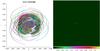 |
Fig. 2 Left: (u,v) coverage of MeerKAT for 8 h of observations, colors correspond to the same baseline. Right: its corresponding PSF. |
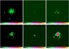 |
Fig. 3 Top: simulated galaxy cluster data. Bottom: simulated M 31 data. From left to right: input images of size 512 × 512 pixels (shown respectively on log scale for the galaxy cluster and linear scale for M 31), dirty images of size 2048 × 2048 pixels and zoom on their central regions of size 512 × 512 pixels. |
The uv-coverage and corresponding PSF of the simulated observations are shown in Fig. 2. The main lobe of the PSF is approximated by a Gaussian clean beam (10.5 × 9.9 arcsec, PA = −28 deg). The resulting dirty images provided by MeqTrees are shown in the middle panel of Fig. 3.
Owing to the important dynamic range (≈1:10 000) of the cluster model map, the diffuse radio emission of the radio halo in the dirty map is completely buried into the PSF side lobes of bright sources (see top panel of Fig. 3). To perform the deconvolution step with MORESANE, we consider the following entries. The gain factor γ that controls the decrease of the residual is set to γ = 0.2. The parameter τ that controls the number of detected objects per iteration is set to τ = 0.7 and the maximum number of iterations to Nitr = 200 and ε = 0.0001. For the wavelets denoising, we use 4σ clipping. For the minor cycle, we fix the maximum number of iterations in the extended gradient conjugate Litr to 50, (tests have shown that convergence is usually reached before) and the precision parameter ϵ to 0.001. MORESANE stops at J = 7. For both Högbom and Multiscale CLEAN tests, we set γ = 0.2, the threshold to 3σ and the maximum number of iterations to Nitr = 10 000. More specifically to the Multiscale CLEAN, we use seven scales [ 0,2,4,8,16,32,64 ] and γ = 0.2. For the IUWT-based CS, we use its reweighted version implemented in MATLAB6. We set the level of the IUWT-decomposition to 6, the threshold to 5 percent of the maximum value in the Fourier transform of the PSF,the regularization parameter λ = 10-8, the threshold to 3σ and the maximum number of iteration Nitr = 50.
The dirty image corresponding to M 31 is displayed in the bottom panel of Fig. 3. The source is completely resolved and above the noise level. To deconvolve it, we set the parameters of MORESANE to τ = 0.7, γ = 0.2, Nitr = 200, ε = 0.0005, and 5σ clipping on the wavelet domain. In the minor loop, we set the precision parameter ϵ = 0.01. MORESANE stops at J = 7. In the case of the Högbom CLEAN, we set γ = 0.2, Nitr = 10 000, and a 3σ threshold. For Multi-Scale CLEAN we adopt: γ = 0.2, Nitr = 10 000, a 3σ threshold and seven scales ([ 0,2,4,8,16,32,64 ]). Finally, the parameters set for the IUWT-based CS method are: seven scales, the threshold to 5 percent of the maximum value in the Fourier transform of the PSF, λ = 10-4, the threshold to 3σ, and the maximum number of iterationNitr = 50.
To numerically quantify the quality of the image recovery by MORESANE with respect to the benchmark algorithms, in terms of fidelity and dynamic range, we use two indicators described in the following.
- i)
The signal-to-noise ratio (S/N) is defined as the ratio of the standard deviation σx of the original sky to the standard deviation
 of the estimated model from the original sky:
 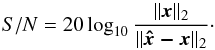 (17)
(17)
 |
Fig. 4 Left: considered uv-coverage; middle and right: dirty images corresponding to the galaxy cluster and M 31, respectively. |
Numerical comparison of the different deconvolution algorithms for the realistic simulations.
Radio astronomers usually refer to the restored map  given by
  (18)where B is the convolution matrix by the clean beam and r is the residual image of the deconvolution.
- ii)
The dynamic range metric (DR) is defined in 34, as the ratio of the peak brightness of the restored image to the standard deviation σr of the residual image,
 (19)
(19)
For a more quantitative comparison between the different methods, we compared the photometry of the reconstructed models versus the true sky. In the case of the galaxy cluster, the total flux density of the true sky over the central 512 × 512 pixel area is 4.10 × 10⁻³ Jy. The total flux values that we get in the cases of Högbom CLEAN, Multi-scale CLEAN, IUWT-based CS, and MORESANE are 3.4 × 10⁻³, 3.6 × 10⁻³, 8.3 × 10⁻³, and 4 × 10⁻³, respectively. We also compared the photometry pixel by pixel as shown in Fig. 7, where we plot the estimated model images on the y-axis against the true sky image on the x-axis. In both tests, MORESANE is the method that gives better results in terms of total flux and surface brightness. MORESANE also gives better results in terms of S/N on the beamed models introduced before (see top part of Table 1).
The results of M 31 reconstruction confirm the better performance of MORESANE. In Fig. 6, we do not show the beamed models where the differences, unlike for the non-beamed versions, are negligible. Instead, we show both the error images  (Fig. 6b) and its beamed version
  (Fig. 6c). While the IUWT-based CS gives a very good estimation of the model source, as confirmed by inspection of Figs. 6a and 8, it is still less competitive than MORESANE when comparing fidelity tests and dynamic range results (bottom part of Table 1). This is strongly related to false detections. The total flux of the sky image is 1495.33 Jy. The reconstructed total flux by Högbom CLEAN, Multi-scale CLEAN, IUWT-based CS, and MORESANE are 1495, 1495.7, 1533, and 1495.8, respectively. Both MORESANE and CLEAN conserve very well the flux, while the high false detection rate of the IUWT-based CS method explains its higher total flux value.
Numerical comparison of SARA and MORESANE for the toy simulations.
6.2. Results for simplified simulations of observations
To compare the performance of MORESANE with the algorithm SARA, we used toy simulations of radio interferometric images, where the considered uv-coverage is a binary sampling function. The latter is derived from the previously generated PSF of MeerKAT. Considering the central part of the PSF of size 512 × 512 pixels, Fourier samples with very low magnitude (< 0.01 of the maximum) are set to zero, as is the central frequency. The remaining values are set to 1, keeping only 4% of the measurements. The resulting new PSF is simply the inverse Fourier transform of the new uv-coverage. Within this configuration, simulated radio images corresponding to the galaxy cluster and M 31 are shown in Fig. 4. An additive white noise of standard deviation 6 × 10⁻⁸ Jy/pixel is added to the visibilities in order to mimic a similar noise level to the previous simulations.
The SARA algorithm has shown its superiority to the IUWT-CS-based algorithm in Carrillo et al. . Therefore, in this paragraph the performance of MORESANE is studied with respect to SARA alone. To do so, we used the MATLAB code of the SARA algorithm7. In this set of simulations, visibilities lie on a perfect grid.MORESANE results are obtained using the same parameters as for the preceding test.
Deconvolution results for the galaxy cluster are shown in Fig. 9. Clearly MORESANE provides a better model than SARA, as confirmed numerically in Table 2. The total flux density of the true sky is 4.10 × 10⁻³ Jy. The total flux values that we get in the cases of SARA and MORESANE are 4.32 × 10⁻³ and 4 × 10⁻³, respectively. In the case of M 31 reconstruction, SARA has proved to perform better deconvolution than MORESANE, as shown in Fig. 10. The total flux of the sky image is 1495.33 Jy, and its estimated values by SARA and MORESANE are 1496.1 and 1496.7. Furthermore, SARA provides better DR and S/N.
In SARA, very faint false components are reconstructed all over the field. Our understanding of this effect is that the method minimizes the difference between the observed and modeled visibilities within an uncertainty range, which is defined inside the algorithm with respect to the noise level. Small errors in the modeled visibilities give rise to weak fluctuations within the whole reconstructed image (in this case a factor of ≈0.01 lower than the minimum surface brightness of the source). The SARA estimated model is the one that describes the visibilities best, within an error margin and subject to an analysis-sparse regularization. This strategy results here in a residual image with very low standard deviation, despite the artifacts visible all over the field (see Fig. 11, middle panel).
The righthand panel of Fig. 11 shows that MORESANE model includes a weak (a factor of ≈0.1 lower than the minimum surface brightness of the source) fake emission at the edge locations of M 31. Because MORESANE uses dictionaries based on isotropic wavelets, edges are less well preserved in the current case where the source is fully resolved, extended, and significantly above the noise level. On the other hand, the MORESANE method does not produce false detections in the field surrounding the source, because source detection (Algorithm 1) and reconstruction (Algorithm 2) are done locally in the wavelet and image domains, respectively.
7. Summary and conclusions
In this paper, we present a new radio deconvolution algorithm – named MORESANE (MOdel REconstruction by Synthesis-ANalysis Estimators) – that combines complementary types of sparse recovery methods in order to reconstruct the most appropriate sky model from observed radio visibilities. A synthesis approach is used for reconstructing images, in which the unknown synthesis objects are learned using analysis priors.
The algorithm has been conceived and optimized for restoring faint diffuse astronomical sources buried in the PSF side lobes of bright radio sources in the field. A typical example of important astrophysical interest is the case of galaxy clusters, which are known to host bright radio objects (extended or unresolved radio galaxies) and low-surface brightness Mpc-scale radio sources ≈ μJy/arcsec2 at 1.4 GHz, 25.
To test MORESANE capabilities, in this paper we simulated realistic radio interferometric observations of known images, in such a way as to be able to directly compare the reconstructed image to the original model sky. Observations performed with the MeerKAT array (i.e., one of the main SKA pathfinders, which is being built in South Africa) were simulated using the MeqTrees software 44. We considered two sky models, including the image of an HII region in M 31, which has been widely adopted in most of previous deconvolution studies, and a model image of a typical galaxy cluster at radio wavelengths, which has been produced using the FARADAY tool 43. We then compared MORESANE deconvolution results to those obtainedby available tools that can be directly applied to radio measurement sets, i.e.,the classical CLEAN and its multiscale variant 14 and one of the novel compressed sensing approaches, the IUWT-based CS method by Li et al. .
Our results indicate that MORESANE is able to efficiently reconstruct images of a wide variety of sources (compact point-like objects, extended tailed radio galaxies, and low-surface brightness emission) from radio interferometric data. In agreement with the conclusions based on other CS-based algorithms e.g., 34; 28, the MORESANE output model has a higher resolution than CLEAN-based methods (compare, e.g., the second and fourth images in the first column of Fig. 5) and represents an excellent approximation of the scene injected in the simulations.
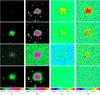 |
Fig. 5 Reconstructed images of the galaxy cluster observations simulated with MeerKAT. The results are shown from top to bottom for Högbom CLEAN, Multi-scale CLEAN, IUWT-based CS and MORESANE. From left to right, model images a), beamed images b), error images of the beamed models with respect to the beamed true sky c) and residual images d). |
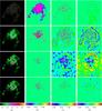 |
Fig. 6 Reconstructed images of M 31 observations simulated with MeerKAT. The results are shown from top to bottom for Högbom CLEAN, Multi-scale CLEAN, IUWT-based CS and MORESANE. From left to right, model images a), error images of the model images with respect to the input image b), error images of the beamed models with respect to the beamed sky image c) and residual images d). |
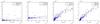 |
Fig. 7 From left to right: results of the galaxy cluster recovery using Högbom CLEAN, MS-CLEAN, IUWT-based CS and MORESANE. Plots of the model images (y-axis) against the input sky image (x-axis). |
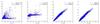 |
Fig. 8 From left to right: results of M 31 recovery using Högbom CLEAN, MS-CLEAN, IUWT-based CS and MORESANE. Plots of the model images (y-axis) against the input sky image (x-axis). |
 |
Fig. 9 Reconstructed images of the galaxy cluster toy simulations. The results are shown for SARA (top) and MORESANE (bottom). From left to right, model images a), beamed images b), error images of the beamed models with respect to the beamed true sky c) and residual images d). |
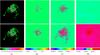 |
Fig. 10 Reconstructed images of M 31 toy simulations. The results are shown for SARA (top) and MORESANE (bottom). From left to right, model images a), error images of the model images with respect to the input image b), error images of the beamed models with respect to the beamed sky image c), and residual images d). |
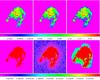 |
Fig. 11 From left to right, input model image of M 31 and reconstructed models by SARA and MORESANE on a log scale, respectively. The figures in the top and bottom lines show exactly the same images, but with different flux contrasts to highlight features within the source and its background. |
Results obtained in the galaxy cluster case (Figs. 5 and 9), as well as the fidelity tests summarized in the top part of Tables 1 and 2, clearly indicate that MORESANE provides a better approximation of the original scene than the other deconvolution methods. In both sets of simulations, the new algorithm proved to be more robust to false detections: while multiscale CLEAN, the IUWT-based CS, and SARA methods detect a large number of fake components, almost all objects in the MORESANE model correspond to genuine sources when checked against the true image. In addition, MORESANE gives better results when comparing the correspondence between the true sky pixels and those reconstructed (see Fig. 7). This proves that MORESANE is robust in the case of a noise level that is significantly higher than the weakest source brightness in the field. These are valuable results for getting an output catalog of sources from radio maps. New radio surveys coming from SKA and its pathfinders will allow getting all-sky images at (sub-)mJy level, thus requiring extremely efficient and reliable source extraction methods 45, and references therein. In addition, thanks to the huge data rate of the new generation of radio telescopes (300 Gigabytes per second in the case of LOFAR, which will increase by a factor of at least one hundred with SKA), observations will not be systematically stored, but data reduction will have to be completely automatized and done on the fly. We plan to develop MORESANE further to automatically extract an output catalog of sources (position, size, flux, etc.) from its reconstructed model. This would allow our new image reconstruction method in pipelines to be easily inserted for automatic data reduction, based also on the fact that our tests indicate that, unlike the IUWT-CS method, the settings of parameters of MORESANE do not need a fine tuning of the user, but can be easily optimized for generalized cases.
The results of M 31 reconstruction are less conclusive for the best deconvolution method. On the realistic simulations, while the IUWT-based CS gives a very good estimation of the model source, it is still less competitive than MORESANE when comparing fidelity tests and dynamic range results owing to the high rate of false model components. However, for the toy simulations of M 31, SARA outperformed MORESANE with a higher dynamic range and fidelity. In the considered M 31 toy model, the source is fully resolved and has a lower noise level than the intensity of its weakest component. We stress here that in true observations, these criteria are only met when observing bright sources with long exposure times and within small filed of views.
These results are extremely encouraging for the application of MORESANE to radio interferometric data. Further developments are planned, including comparing our tool to other existing algorithms that are, for the moment, not publicly available e.g., 28, taking the variations in the PSF across the field-of-view of the instrument into account, studying other possible analysis dictionaries, reconstructing spectral images, and testing performances on poorly calibrated data. Tests of MORESANE on real observations, which will be the object of a separate paper, are ongoing and promising. The results of this paper were obtained by using MORESANE in its original version written in MATLAB. PyMORESANE, a recently developed Python implementation of MORESANE8, is now freely available to the community under the GPL2 license9. PyMORESANE is a self-contained tool that includes GPU (CUDA) acceleration and that can be used on large datasets, within an execution time that is comparable to the standard image reconstruction tools.
For a vector x,  .
.
MFS is assumed to have unit-norm ℓ2 columns. If this is not the case, the components of  should be weighted accordingly see, e.g., 4.
See for instance the references of http://small-project.eu/publications
Found at https://github.com/basp-group/sopt
The implementation only depends on the most common Python modules, in particular SciPy, NumPy, and PyFITS.
Acknowledgments
We warmly thank Huib Intema for very helpful comments, and Federica Govoni and Matteo Murgia for providing the galaxy cluster simulated radio map analyzed in this paper. We acknowledge financial support by the Agence Nationale de la Recherche through grants ANR-09-JCJC-0001-01 Opales and ANR-14-CE23-0004-01 Magellan, the PHC PROTEA programme (2013) through grant 29732YK, the joint doctoral program région PACA-OCA, and Thales Alenia Space (2011).
References
- Arias-Castro, E., Candès, E. J., & Plan, Y. 2010, Ann. Stat., 39, 2533 [Google Scholar]
- Beck, R., & Reich, W. 1985, in The Milky Way Galaxy, eds. H. van Woerden, R. J. Allen, & W. B. Burton, IAU Symp., 106, 239 [Google Scholar]
- Biemond, J., Lagendijk, R., & Mersereau, R. 1990, Proc. IEEE, 78, 856 [CrossRef] [Google Scholar]
- Bourguignon, S., Mary, D., & Slezak, É. 2011, IEEE J. Selected Topics in Signal Processing, 5, 1002 [NASA ADS] [CrossRef] [Google Scholar]
- Bozzetto, L. M., Filipović, M. D., Urošević, D., Kothes, R., & Crawford, E. J. 2014, MNRAS, 440, 3220 [NASA ADS] [CrossRef] [Google Scholar]
- Briggs, D. S., Schwab, F. R., & Sramek, R. A. 1999, in Synthesis Imaging in Radio Astronomy II, eds. G. B. Taylor, C. L. Carilli, & R. A. Perley, ASP Conf. Ser., 180, 127 [Google Scholar]
- Brunetti, G., & Jones, T. W. 2014, Int. J. Mod. Phys. D, 23, 30007 [Google Scholar]
- Candès, E., & Donoho, D. 1999, Phil. Trans. R. Soc. Lond. A., 357, 2495 [Google Scholar]
- Candès, E. J., Romberg, J., & Tao, T. 2006, IEEE Trans. Information Theory, 52, 489 [CrossRef] [Google Scholar]
- Carlavan, M., Weiss, P., & Blanc-Féraud, L. 2010, Traitement du signal, 27, 189 [CrossRef] [Google Scholar]
- Carrillo, R. E., McEwen, J. D., & Wiaux, Y. 2012, MNRAS, 426, 1223 [NASA ADS] [CrossRef] [MathSciNet] [Google Scholar]
- Carrillo, R. E., McEwen, J. D., & Wiaux, Y. 2013, MNRAS, submitted [Google Scholar]
- Chen, S. S., Donoho, D. L., & Saunders, M. A. 1998, SIAM J. Sci. Comput., 20, 33 [Google Scholar]
- Cornwell, T. J. 2008, IEEE J. Selected Topics in Signal Processing, 2, 793 [Google Scholar]
- Cornwell, T. 2009, A&A, 500, 65 [NASA ADS] [CrossRef] [EDP Sciences] [Google Scholar]
- Dabbech, A., Mary, D., & Ferrari, C. 2012, in IEEE Int. Conf. on Acoustics, Speech and Signal Processing (ICASSP), 3665 [Google Scholar]
- de Gasperin, F., Orrú, E., Murgia, M., et al. 2012, A&A, 547, A56 [NASA ADS] [CrossRef] [EDP Sciences] [Google Scholar]
- Donoho, D. L. 2006, IEEE Trans. Information Theory, 52, 1289 [CrossRef] [Google Scholar]
- Donoho, D., & Huo, X. 2001, IEEE Trans. Information Theory, 47, 2845 [CrossRef] [Google Scholar]
- Donoho, D. L., & Johnstone, I. M. 1994, Biometrika, 81, 425 [CrossRef] [MathSciNet] [Google Scholar]
- Donoho, D. L., Tsaig, Y., Drori, & Starck, J. 2006, Sparse Solution of Underdetermined Linear Equations by Stagewise Orthogonal Matching Pursuit, Tech. Rep., Stanford University, IEEE Trans. Information Theory, submitted [Google Scholar]
- Elad, M., Milanfar, P., & Rubinstein, R. 2007, Inverse Problems, 23, 947 [NASA ADS] [CrossRef] [Google Scholar]
- Feretti, L., & Venturi, T. 2002, in Merging Processes in Galaxy Clusters, eds. L. Feretti, I. M. Gioia, & G. Giovannini, Astrophys. Space Sci. Lib., 272, 163 [Google Scholar]
- Feretti, L., Giovannini, G., Govoni, F., & Murgia, M. 2012, A&ARv, 20, 54 [Google Scholar]
- Ferrari, C., Govoni, F., Schindler, S., Bykov, A. M., & Rephaeli, Y. 2008, Space Sci. Rev., 134, 93 [NASA ADS] [CrossRef] [Google Scholar]
- Fomalont, E. B., & Perley, R. A. 1999, in Synthesis Imaging in Radio Astronomy II, eds. G. B. Taylor, C. L. Carilli, & R. A. Perley, ASP Conf. Ser., 180, 79 [Google Scholar]
- Friedman, J. H., & Stuetzle, W. 1981, J. Am. Statistical Association, 76, 817 [Google Scholar]
- Garsden, H., Girard, J. N., Starck, J. L., et al. 2015, A&A, 575, A90 [NASA ADS] [CrossRef] [EDP Sciences] [Google Scholar]
- Giovannelli, J.-F., & Coulais, A. 2005, A&A, 439, 401 [NASA ADS] [CrossRef] [EDP Sciences] [Google Scholar]
- Govoni, F., Murgia, M., Feretti, L., et al. 2006, A&A, 460, 425 [NASA ADS] [CrossRef] [EDP Sciences] [Google Scholar]
- Gribonval, R., & Nielsen, M. 2003, IEEE Trans. Information Theory, 49, 3320 [CrossRef] [Google Scholar]
- Högbom, J. A. 1974, A&AS, 15, 417 [NASA ADS] [Google Scholar]
- Johnstone, I. M., & Silverman, B. W. 1997, J. Roy. Statistical Society: Series B (Stat. Method.), 59, 319 [CrossRef] [Google Scholar]
- Li, F., Cornwell, T. J., & de Hoog, F. 2011, A&A, 528, A31 [NASA ADS] [CrossRef] [EDP Sciences] [Google Scholar]
- Magain, P., Courbin, F., & Sohy, S. 1998, ApJ, 494, 472 [NASA ADS] [CrossRef] [Google Scholar]
- Mallat, S. 2008, A Wavelet Tour of Signal Processing, The Sparse Way, 3rd edn. (Academic Press) [Google Scholar]
- Mallat, S., & Zhang, Z. 1993, IEEE Trans. Signal Processing, 41, 3397 [CrossRef] [Google Scholar]
- Mary, D. 2009, in Conference on Advanced Inverse Problems, Vienna, http://www.ricam.oeaw.ac.at/conferences/aip2009/minisymposia/slides/aip2009_m20_mary_david.pdf [Google Scholar]
- Mary, D., &Michel, O. 2007, in XXI Colloque GRETSI, http://documents.irevues.inist.fr/bitstream/handle/2042/17610/GRE...?sequence=1, SS1–3.9 [Google Scholar]
- Mary, D., Valat, B., Michel, O., F. X., S., & Lopez, B. 2008, in 5th Conference on Astronomical Data Analysis, (ADA 5), Heraklion, Crete, http://www.ics.forth.gr/ada5/pdf_files/Mary_poster.pdf [Google Scholar]
- Mary, D., Bourguignon, S., Theys, C., & Lanteri, H. 2010, in ADA 6 – Sixth Conference on Astronomical Data Analysis, http://ada6.cosmostat.org/Presentations/PresADA6_Mary.pdf [Google Scholar]
- McEwen, J. D., & Wiaux, Y. 2011, MNRAS, 413, 1318 [NASA ADS] [CrossRef] [Google Scholar]
- Murgia, M., Govoni, F., Feretti, L., et al. 2004, A&A, 424, 429 [NASA ADS] [CrossRef] [EDP Sciences] [Google Scholar]
- Noordam, J. E., & Smirnov, O. M. 2010, A&A, 524, A61 [NASA ADS] [CrossRef] [EDP Sciences] [Google Scholar]
- Norris, R. P., Afonso, J., Bacon, D., et al. 2013, PASA, 30, 20 [Google Scholar]
- Paladino, R., Murgia, M., Helfer, T. T., et al. 2006, A&A, 456, 847 [NASA ADS] [CrossRef] [EDP Sciences] [Google Scholar]
- Pirzkal, N., Hook, R. N., & Lucy, L. B. 2000, in Astronomical Data Analysis Software and Systems IX, eds. N. Manset, C. Veillet, & D. Crabtree, ASP Conf. Ser., 216, 655 [Google Scholar]
- Réfrégier, A. 2003, MNRAS, 338, 35 [NASA ADS] [CrossRef] [Google Scholar]
- Schwarz, U. 1978, A&A, 65, 417 [Google Scholar]
- Solo, V. 2008, in Proceedings ICASSP, 2008 [Google Scholar]
- Starck, J. L., & Bijaoui, A. 1992, in ESO Conf. and Workshop Proc., Vol. 39, eds. J. M. Beckers, & F. Merkle, 853 [Google Scholar]
- Starck, J., & Murtagh, F. 1994, A&A, 288, 342 [NASA ADS] [Google Scholar]
- Starck, J. L., Pantin, E., & Murtagh, F. 2002, PASP, 114, 1051 [NASA ADS] [CrossRef] [Google Scholar]
- Starck, J. L., Donoho, D. L., & Candès, E. J. 2003, A&A, 398, 785 [NASA ADS] [CrossRef] [EDP Sciences] [Google Scholar]
- Starck, J.-L., Fadili, J., & Murtagh, F. 2007, IEEE Trans. Image Processing, 16, 297 [Google Scholar]
- Starck, J.-L., Murtagh, F., & Fadili, M.-J. 2010, Sparse Image and Signal Processing – Wavelets, Curvelets, Morphological Diversity (Cambridge University Press), 1 [Google Scholar]
- Starck, J.-L., Murtagh, F., & Bertero, M. 2011, in Handbook of Mathematical Methods in Imaging, ed. O. Scherzer (New York: Springer), 1489 [Google Scholar]
- Tasse, C., van der Tol, S., van Zwieten, J., van Diepen, G., & Bhatnagar, S. 2013, A&A, 553, A105 [NASA ADS] [CrossRef] [EDP Sciences] [Google Scholar]
- Thompson, A. R., Moran, J. M., & Swenson, Jr., G. W. 2001, Interferometry and Synthesis in Radio Astronomy, 2nd edn. (New York: Wiley) [Google Scholar]
- van Haarlem, M. P., Wise, M. W., Gunst, A. W., et al. 2013, A&A, 556, A2 [NASA ADS] [CrossRef] [EDP Sciences] [Google Scholar]
- Vannier, M.,Mary, D., Millour, F., et al. 2010, in SPIE Conf. Ser., 7734 [Google Scholar]
- Wakker, B. P., & Schwarz, U. J. 1988, A&A, 200, 312 [NASA ADS] [Google Scholar]
- Wenger, S., Darabi, S., Sen, P., Glassmeier, K.-H., & Magnor, M. 2010, in Proc. IEEE Int. Conf. Image Processing (ICIP) 2010, 1381 [Google Scholar]
- Wiaux, Y., Jacques, L., Puy, G., Scaife, A. M. M., & Vandergheynst, P. 2009, MNRAS, 395, 1733 [NASA ADS] [CrossRef] [Google Scholar]
- Wiaux, Y., Puy, G., Boursier, Y., & Vandergheynst, P. 2009, MNRAS, 400, 1029 [NASA ADS] [CrossRef] [Google Scholar]
All Tables
Numerical comparison of the different deconvolution algorithms for the realistic simulations.
All Figures
|
Fig. 1 Bottom right: a galaxy cluster model image, with a galaxy circled in yellow. From top left to bottom middle: IUWT analysis coefficients |
| In the text | |
|
Fig. 2 Left: (u,v) coverage of MeerKAT for 8 h of observations, colors correspond to the same baseline. Right: its corresponding PSF. |
| In the text | |
|
Fig. 3 Top: simulated galaxy cluster data. Bottom: simulated M 31 data. From left to right: input images of size 512 × 512 pixels (shown respectively on log scale for the galaxy cluster and linear scale for M 31), dirty images of size 2048 × 2048 pixels and zoom on their central regions of size 512 × 512 pixels. |
| In the text | |
|
Fig. 4 Left: considered uv-coverage; middle and right: dirty images corresponding to the galaxy cluster and M 31, respectively. |
| In the text | |
|
Fig. 5 Reconstructed images of the galaxy cluster observations simulated with MeerKAT. The results are shown from top to bottom for Högbom CLEAN, Multi-scale CLEAN, IUWT-based CS and MORESANE. From left to right, model images a), beamed images b), error images of the beamed models with respect to the beamed true sky c) and residual images d). |
| In the text | |
|
Fig. 6 Reconstructed images of M 31 observations simulated with MeerKAT. The results are shown from top to bottom for Högbom CLEAN, Multi-scale CLEAN, IUWT-based CS and MORESANE. From left to right, model images a), error images of the model images with respect to the input image b), error images of the beamed models with respect to the beamed sky image c) and residual images d). |
| In the text | |
|
Fig. 7 From left to right: results of the galaxy cluster recovery using Högbom CLEAN, MS-CLEAN, IUWT-based CS and MORESANE. Plots of the model images (y-axis) against the input sky image (x-axis). |
| In the text | |
|
Fig. 8 From left to right: results of M 31 recovery using Högbom CLEAN, MS-CLEAN, IUWT-based CS and MORESANE. Plots of the model images (y-axis) against the input sky image (x-axis). |
| In the text | |
|
Fig. 9 Reconstructed images of the galaxy cluster toy simulations. The results are shown for SARA (top) and MORESANE (bottom). From left to right, model images a), beamed images b), error images of the beamed models with respect to the beamed true sky c) and residual images d). |
| In the text | |
|
Fig. 10 Reconstructed images of M 31 toy simulations. The results are shown for SARA (top) and MORESANE (bottom). From left to right, model images a), error images of the model images with respect to the input image b), error images of the beamed models with respect to the beamed sky image c), and residual images d). |
| In the text | |
|
Fig. 11 From left to right, input model image of M 31 and reconstructed models by SARA and MORESANE on a log scale, respectively. The figures in the top and bottom lines show exactly the same images, but with different flux contrasts to highlight features within the source and its background. |
| In the text | |
Current usage metrics show cumulative count of Article Views (full-text article views including HTML views, PDF and ePub downloads, according to the available data) and Abstracts Views on Vision4Press platform.
Data correspond to usage on the plateform after 2015. The current usage metrics is available 48-96 hours after online publication and is updated daily on week days.
Initial download of the metrics may take a while.