| Issue |
A&A
Volume 575, March 2015
|
|
|---|---|---|
| Article Number | A73 | |
| Number of page(s) | 6 | |
| Section | Catalogs and data | |
| DOI | https://doi.org/10.1051/0004-6361/201425605 | |
| Published online | 26 February 2015 | |
Cassini ISS astrometry of the Saturnian satellites: Tethys, Dione, Rhea, Iapetus, and Phoebe 2004–2012⋆
1
IMCCE, Observatoire de Paris, UMR 8028 du CNRS, UPMC, Université de Lille
1,
77 av. Denfert-Rochereau,
75014
Paris,
France
2
Department of Astronomy, Cornell University,
326 Space Sciences Building,
Ithaca, NY
14853,
USA
e-mail:
tajeddine@astro.cornell.edu
3
Astronomy Unit, Queen Mary University of London,
Mile End Road, London
E1 4NS,
UK
Received: 31 December 2014
Accepted: 19 January 2015
Context. The Cassini spacecraft has been orbiting Saturn since 2004 and has returned images of satellites with an astrometric resolution as high as a few hundred meters per pixel.
Aims. We used the images taken by the Narrow Angle Camera (NAC) of the Image Science Subsystem (ISS) instrument on board Cassini, for the purpose of astrometry.
Methods. We applied the same method that was previously developed to reduce Cassini NAC images of Mimas and Enceladus.
Results. We provide 5463 astrometric positions in right ascension and declination (α, δ) of the satellites: Tethys, Dione, Rhea, Iapetus, and Phoebe, using images that were taken by Cassini NAC between 2004 and 2012. the mean residuals compared to the JPL ephemeris SAT365 are of the order of hundreds of meters with standard deviations of the order of a few kilometers. The frequency analysis of the residuals shows the remaining unmodelled effects of satellites on the dynamics of other satellites.
Key words: astrometry / planets and satellites: individual: Tethys / planets and satellites: individual: Dione / planets and satellites: individual: Rhea / planets and satellites: individual: Iapetus / planets and satellites: individual: Phoebe
Full Table 1 is only available at the CDS via anonymous ftp to cdsarc.u-strasbg.fr (130.79.128.5) or via http://cdsarc.u-strasbg.fr/viz-bin/qcat?J/A+A/575/A73
© ESO, 2015
1. Introduction
The origin and orbital evolution of the Saturnian moons has long been a debated topic. The intensity of the tides that are the main driver for orbital migration are usually described at first order by the Love number k2 (set to 0.341, Gavrilov & Zharkov 1977) and the quality factor Q. While the dissipation factor of Saturn has been estimated in the past to be Q = 18 000 (Sinclair 1983), Lainey et al. (2012) reported a new value of Q = 1682 ± 540 based on Hubble Space Telescope (HST) and ground-based astrometry from over a century of observations, yielding a fast expansion of the satellites’ semi-major axes. This new result allows a recently published model Charnoz et al. (2011), which forms the mid-sized moons in the rings, to place the moons at their current distances from Saturn, contrary to the classic models that form the main moons in the subnebula of Saturn (Canup & Ward 2002, 2006; Mosqueira & Estrada 2003, 2003; Sasaki et al. 2010; Sekine & Genda 2012), which raises the question how old the rings and moons of Saturn are. On the other hand, the interiors of the Saturnian satellites are still not entirely understood. Some suggest that there is an internal global ocean under Enceladus’ icy shell (Nimmo & Pappalardo 2006; Lainey et al. 2012), others suggest a subsurface “sea” localized in its south polar region (Collins & Goodman 2007; Iess et al. 2014). Meanwhile, the physical forced libration measurements (Tajeddine et al. 2014) suggest that Mimas has a more complex interior than was previously believed and may have a subsurface ocean.
Spacecraft astrometry has proven to be an indispensable tool for accurate orbit modelling, and many spacecraft images were used for the purpose of astrometry. For instance, from Voyager 2 optical images, Jacobson (1991, 1992) provided astrometric positions of the Neptunian and Uranian main satellites. Mars Express observations were used to reduce the positions of the Martian satellites Phobos and Deimos (Willner et al. 2008, Pasewaldt et al. 2012). Cassini ISS observations have also been used for astrometric reduction; Cooper et al. (2006) modelled the orbits of the Jovian moons Amalthea and Thebe, Tajeddine et al. (2013) provided astrometric positions of Mimas and Enceladus, Cooper et al. (2014) presented astrometry of the small inner moons of Saturn, Atlas, Prometheus, Pandora, Janus, and Epimetheus, Cooper et al. (2014) reduced mutual-event observations of the mid-sized icy moons of Saturn, and Desmars et al. (2013) used the astrometric positions presented in this paper to model the orbit of Phoebe. The reduction of Cassini observations has provided very accurate astrometric positions of satellites that can reach a low error of one kilometer at times. This accuracy of astrometry is essential to answer questions related to the origin and orbital evolution of the satellites.
Sample of the results given by the astrometric reduction.
In this work we provide a total number of 5240 astrometric positions of the Saturnian moons Tethys, Dione, Rhea, and Iapetus using Cassini ISS NAC images taken during the period of 2004–2012. We also reduced 223 observations of Phoebe taken during a seven-day flyby from 6 and 13 June 2004 upon Cassini’s orbit insertion around the system of Saturn. This paper is an application of and a follow up work to the previously published Cassini astrometry on Mimas and Enceladus (Tajeddine et al. 2013). Astrometry for Titan and Hyperion is not given here because of the former’s atmosphere and the latter’s chaotic rotation, which both affect the centre of figure-finding.
The method for astrometry previously developed by Tajeddine et al. (2013) is briefly recalled in Sect. 2. A sample of the astrometric observations and an analysis of the residuals are given in Sect. 3. We conclude in Sect. 4.
2. Method
All the Cassini ISS NAC images were downloaded from the Planetary Data System (PDS) website1. Each image was first submitted to photometric calibration with the software CISSCAL (West et al. 2010). We extracted the mid-time in UTC of each observation from the image’s header. Using the available online SPICE library2 (Acton 1996) we determined the right ascension and declination (αc,δc) of the NAC centre of the field of view. The Cassini camera orientation and its field of view are useful to know which stars are expected to be seen in the image. We used the UCAC2 star catalogue (Zacharias et al. 2004) as a reference for camera-pointing correction. The stellar right ascension and declination (α∗,δ∗) in this catalogue are given in the International Celestial Reference Frame (ICRF).
The astrometric reduction model we developed consists of the following: the stellar coordinates (α∗,δ∗) are first corrected for proper motion, aberration, relativistic effects, and change of the observer location from the solar system barycentre to the Cassini spacecraft (Kaplan et al. 1989). These coordinates are then converted using gnomonic projection from the celestial sphere (with a field of view of ≈0.35° × 0.35°) to the tangential coordinates (X,Y) on the camera CCD plane (Eichhorn 1974). These coordinates are then converted into the camera as sample and line coordinates using the NAC scale factor and twist angle θ (known within 90 μrad of error, Tajeddine et al. 2013).
With this model, the NAC pointing correction was achieved by fitting the positions of the catalogue stars (projected onto the image) to the detected ones. Stellar detection was made using the IDL3-based routine “FIND” (Stetson 1987), which searches (pixel by pixel) for Gaussian signals in the image.
The next step is measuring the satellite centre of figure; for the good resolution of Cassini images, a limb can be measured. To do so, we measured the limb by searching the highest absolute value of the derivative of the pixel intensity plots. We then projected the satellite’s three-dimensional ellipsoidal shape given by Thomas (2010) onto the image and adjusted the projected ellipse to the measured limb points. We typically fitted five parameters of the ellipse, the center sample and line (s,l) coordinates, the semi-major and semi-minor axes, and the ellipse orientation. The ellipse axes are fixed by the projection onto the image, and its orientation is fixed by the satellite known orientation of the poles (Archinal et al. 2011), and the camera twist angle, which leaves the ellipse sample and line (s,l) coordinates to be fitted; these represent the pixel coordinates of the satellite on the image. After measuring the satellite imaged position in sample and line (s,l), right ascension (αs) and declination (δs) are obtained by inverting the transformations described above. For more details on the astrometric model we used, the limb measurement, ellipse fitting methods, and the comparison with the classical model, we refer to Tajeddine et al. (2013).
3. Astrometric observations
A total number of 5463 astrometric positions of the satellites Tethys, Dione, Rhea, Iapetus, and Phoebe were reduced, applying the method described in the previous section. Table 1 gives a sample of the complete set of reduced observations, which are available on the CDS website. The variables in this table are described as follows: image name, date and exposure mid-time of the image (UTC), satellite name, right ascension and declination of the satellite (in the ICRF), observation uncertainties in right ascension and declination, right ascension and declination of the camera pointing vector, twist angle (defined in Tajeddine et al. 2013), sample and line (in pixels) of the observed satellite in the image, and finally the number of the detected stars in the image. All the angle variables are given in degrees. Note that the image sample coordinates are reversed compared to those given by Cooper et al. (2014) because of a difference in the definition of the sample and line origin. Figure 1 shows a small sample of the reduced images.
This work and the previous ones (Tajeddine et al. 2013; Cooper et al. 2014) do not provide the Cassini astrometry of Titan because its atmosphere prevents determining its shape or the location of its limb, therefore the astrometric positions are inaccurate. Hence, more complex limb detection and fitting methods need to be developed for this satellite. The astrometric positions of Hyperion are not given either. Its irregular shape is problematic for limb fitting, but this problem can be solved with the ellipsoidal approximation as we did for Phoebe (Fig. 1e). The chaotic rotation is the most difficult problem for Hyperion because its orientation (relative to Cassini) is unpredictable, which makes it impossible to know which part of the ellipsoid is to be projected onto the CCD plane. The only solution would be fitting all the five parameters of the ellipsoid to only one visible limb of an irregular body, which would increase the errors on the astrometric positions to a few tens of kilometers.
Tethys, Dione, and Rhea were less of a challenge for Cassini astrometry. Their surfaces are smooth enough for limb measurement and centre-of-figure finding, although the larger the satellite, the lower its resolution since the whole satellite has to be seen in the field of view plus the background sky for star detection.
The “two-faced” surface of Iapetus (Fig. 1d) was challenging, however; either the exposure time was short enough to make the surface patterns on the bright side visible, but too short to measure the limb on the dark side, or it was long enough to make the surface patterns on the dark side visible, but too long so that the limb on the bright side seemed larger. The best images for Iapetus astrometry are when the spacecraft is observing one side at a time.
Lastly, the center-of-figure finding for Phoebe was the most complicated of all. Its shape is so irregular (Fig. 1e) that limb detection was very difficult especially near the terminator where any topographic elevation can be taken for a limb point; sometimes the maximum of the light change is not located at the limb but at a crater on the satellite which can trick the limb detection program. In addition, fitting an ellipsoid to such an irregular shape does not provide the best astrometry. The best solution would be to build a 3D model of Phoebe based on a high order of spherical harmonics expansion similar to the work done on Phobos (Willner et al. 2014). Phoebe was only observed in high resolution during the seven days of the Cassini flyby in June 2004 immediately before orbit insertion. Because it is very far from Saturn, it will not be observed in high resolution by the Cassini spacecraft again. These observations have already been used by Desmars et al. (2013) to study the orbit of Phoebe.
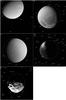 |
Fig. 1 Sample of the reduced images of a) Tethys; b) Dione; c) Rhea; d) Iapetus; e) Phoebe. Expected and measured positions of UCAC2 stars are superimposed on the images. |
3.1. Analysis of the residuals
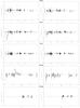 |
Fig. 2 Residuals of Tethys, Dione, Rhea, Iapetus, and Rhea to SAT365 ephemeris in αcosδ and δ, converted to kilometers. For Phoebe, day 0 represents 6 June 2004. |
Figure 2 shows the residuals relative to the JPL ephemeris SAT365 in right ascension (αcosδ) and declination (δ) converted into kilometers as a function of time. Mean values and standard deviations of residuals are given in Table 2. The residuals are given in kilometers and not in angle units or image pixels because the distance between the spacecraft and the satellite vary significantly from one image to another, which in turn varies the image resolution; the same applies to angle units. Therefore, giving the residuals in pixels or in angle units is not as informative as giving them in kilometers. Table 3 shows the percentage of residuals that are lower than their estimated observation uncertainties in αcosδ and δ. If the observation uncertainties were well estimated, one would expect a percentage of about 66.7%. If the percentage were lower than this value, then the uncertainties have been underestimated. If it was greater, then the uncertainties would have been overestimated. The table shows that for Tethys the uncertainties have a good estimation, but they seem to be overestimated for Dione and Rhea. this may be because the uncertainty on each limb point measurement is fixed to 0.5 pixel, and since the surfaces of Dione and Rhea are smoother than that of Tethys, the location of the limb for those two satellites could be known to within less than 0.5 pixels. Tajeddine et al. (2013) have shown that the heavily crated surface of Mimas decreases the accuracy in the center-of-figure measurement, causing an underestimation of the uncertainties. Indeed, the same phenomenon is clearly noticeable for Phoebe, where the uncertainties on the astrometric positions are underestimated. This is due to (as mentioned earlier in Sect. 3) the fit of a regular ellipsoid to an irregular body. For Iapetus, the uncertainties seem to be underestimated as well; one explanation is in the large equatorial ridge that is not included in the shape model; another is the color difference that sometimes tricked the limb measurement, as noted earlier in the same section.
Mean values with standard deviations of residuals with respect to the JPL SAT365 ephemeris.
Percentage of observations with (O−C) lower than the observation uncertainty in αcosδ and in δ.
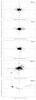 |
Fig. 3 Residuals of Tethys, Dione, Rhea, Iapetus, and Rhea to SAT365 ephemeris in pixel represented in a frame where X-axis is in the Sun direction. |
Cooper et al. (2014) reduced the MUTUALEVE observations, which have a specific geometry in which the phase angle varies by about 90–100 deg and the Sun is always located around the positive line direction. They reported a clear systematic bias in the increasing line direction because only one part of the satellite is observed, which shifts the centre of figure in the same direction. The JPL ephemerides are only based on these types of observations and the those called SATELLORB, which likewise have a specific observation geometry. Here we analysed every Cassini ISS NAC image found in the database4. Some of these observations were originally designed for geological studies where the satellite occupies most of the image, and stellar detection is very difficult in such situations because the stars are either hidden behind the satellite, or the exposure time is too short because of the satellite’s high brightness (as shown by Tajeddine et al. 2013). The image resolution varied between 0.4 km/pix (for a flyby of a moon as small as Phoebe) and 70 km/pix (the poorest resolution of a large moon like Rhea), the phase angle has a wide range of values, resulting in images varying from the barely visible to a full moon, with the Sun in no fixed direction in the images. Figure 3 shows the residuals (in pixels) for all the satellites, represented in a frame where the X-axis is oriented towards the Sun. The figure does not show any obvious bias in the direction of the Sun. One explanation can be that the limb-detection parameters were adjusted to adapt to the variation of the phase angle in different images. For instance, the limb-detection sensitivity for high phase-angle observations was set to a much higher value than of low-phase observations. This does not mean that there is no effect of the Sun on the residuals. Figure 3 shows that the residuals are more widely spread in the solar direction than those orthogonal to the solar direction, and the irregular shape of Phoebe is the best example. Thus, the solar phase angle does affect the astrometric residuals but here it is rather randomized because of the random solar geometry.
3.2. Frequency analysis
The residuals in Fig. 2 were also given in kilometers for the purpose of frequency analysis. We analysed the residuals in right ascension and in declination for all the satellites, using the frequency mapping FAMOUS5. Table 4 shows the results of the analysis for each satellite. All the amplitudes of the detection periods are in order of magnitude of the standard deviation of the residuals (Table 2); this adds noise to the detected signals. Moreover, the larger the satellite, the lower the imaging resolution becomes, which is another source of error in the frequency analysis.
For Tethys, three periods were detected: 1.37 and 1.88 days corresponding to the orbital periods of Enceladus and Tethys, respectively, and the last one of 1.34 days is the beat period (Tbeat) between the orbital period of Tethys (T1) of 1.888 days and the period (T2) of 4.57 days close to the period of Rhea (4.528 days), where the beat period is defined as  (1)For Dione, the strongest signal is recorded for a period of 21.82 days, which is very close the orbital period of Hyperion (21.276 days), followed by a period of 2.75 days, close to the orbital period of Dione (2.737 days). The last signal is the beat period between the orbital period of Dione and the period of 1.88 days, which is the orbital period of Tethys.
For Rhea, two signals were detected. One for a period of 20.15 days that may correspond to the orbital period of Hyperion, the other signal is for a period of 1.31 days, which results in beat period between the orbital period of Rhea and the period of 1.88 days, which again is the orbital period of Tethys.
For Iapetus, the strongest signal has a period of 499.95 days. This may be the orbital period of Phoebe (550.57 days). The last signal has a period of 16.43 days, which results in a beat period between orbital period of Iapetus and the period of 20.71 days that could be the orbital period of Hyperion.
Finally, no periodic signals were found in the residuals of Phoebe which is due to the short observation time and the high residuals.
The frequency analysis of the astrometric residuals shows few possible remaining effects that were not entirely accounted for in the latest (at the time of writing) JPL ephemeris SAT365. In particular, the orbital period of Tethys seems to appear in the residuals of Tethys, Dione, and Rhea.
Frequency analysis of the residuals.
4. Conclusion
We provide astrometric positions of four of the main moons of Saturn: Tethys, Dione, Rhea, and Iapetus, for a time span of 2004–2012. In addition, we reduced the observations of the 7 day flyby of Phoebe in June 2004. The total number of astrometric positions given in this paper is 5463. The residuals to the JPL ephemeris SAT365 are of the order of few kilometers which is an improvement of two orders of magnitude in astrometric accuracy in comparison to earth-based astrometry (where the residuals are in the order of hundreds of kilometers). Unlike Tethys, Dione, and Rhea, the center of figure finding was more complicated for Iapetus (because of the change of colors between the two side), and for Phoebe (because of the fit of a regular ellipsoid to an irregularly shaped body). The astrometric
positions of Titan were not provided because of its atmosphere that prevents the detection of the actual limb of the satellite; this requires a more sophisticated method for limb detection than the one used in this work. The astrometric positions of Hyperion were also not provided because of its chaotic rotation so limb fitting results in astrometric positions that are as bad as selecting the center of figure of the moon manually.
Frequency analysis of the residuals reveals some effects that were not completely accounted for. The orbital period of Enceladus was detected in the residuals of Tethys, which its orbital period was detected in each of the residuals of Tethys, Dione, and Rhea. The orbital period of Dione was detected in the residuals of the same moon. The orbital period of Rhea was detected in the residuals of Tethys. There might be signatures of the orbital period of Hyperion in the residuals of Dione, Rhea, and Iapetus. Finally, the orbital period of Phoebe might also be present in the residuals of Iapetus.
The Cassini spacecraft will continue to orbit Saturn until late 2017 and more data continues to arrive. The astrometric positions published in this paper and the ones that will be obtained in the future are going to be critical for studying the orbital evolution and origin of the system of Saturn.
IDL Astronomy User’s Library URL: http://idlastro.gsfc.nasa.gov/
Planetary Data System (PDS) http://pds.nasa.gov/
Acknowledgments
This work was mainly funded by European Community’s Seventh Framework Program (FP7/2007-2013) under grant agreement 263466 for the FP7-ESPaCE, and partially by UPMC-EMERGENCE (contract number EME0911), for which R.T. and V.L. are grateful. R.T. was also supported by the Cassini mission. In addition, this work was supported by the Science and Technology Facilites Council (Grant No. ST/F007566/1) and C.D.M. and N.J.C. are grateful to them for financial assistance. C.D.M. is also grateful to the Leverhulme Trust for the award of a Research Fellowship. The authors also thank the ESPaCE and Encelade working groups for fruitful discussions and the anonymous referee for the kind comments.
References
- Acton, C. H. 1996, Planet. Space Sci., 44, 65 [NASA ADS] [CrossRef] [Google Scholar]
- Archinal, B. A., A’Hearn, M. F., Bowell, E., et al. 2011, Celest. Mech. Dyn. Astron., 109, 101 [Google Scholar]
- Canup, R. M., & Ward, W. R. 2002, AJ, 124, 3404 [NASA ADS] [CrossRef] [Google Scholar]
- Canup, R. M., & Ward, W. R. 2006, Nature, 441, 834 [NASA ADS] [CrossRef] [Google Scholar]
- Charnoz, S., Crida, A., Castillo-Rogez, J. C., et al. 2011, Icarus, 216, 535 [Google Scholar]
- Collins, G. C., & Goodman, J. C. 2007, Icarus, 189, 72 [NASA ADS] [CrossRef] [Google Scholar]
- Cooper, N. J., Murray, C. D.,Porco, C. C., & Spitale, J. N. 2006, Icarus, 181, 223 [NASA ADS] [CrossRef] [Google Scholar]
- Cooper, N. J., Renner, S., Murray, C. D., & Evans, M. W. 2014a, AJ, 149, 27 [NASA ADS] [CrossRef] [Google Scholar]
- Cooper, N. J., Murray, C. D., Lainey, V., et al. 2014b, A&A, 572, A8 [NASA ADS] [CrossRef] [EDP Sciences] [Google Scholar]
- Desmars, J., Li, S. N., Tajeddine, R., Peng, Q. Y., & Tang, Z. H. 2013, A&A, 553, A10 [Google Scholar]
- Eichhorn, H. 1974, Astrometry of star positions (New York: Frederick Ungar) [Google Scholar]
- Gavrilov, S. V., & Zharkov, V. N. 1977, Icarus, 32, 443 [NASA ADS] [CrossRef] [Google Scholar]
- Iess, L., Stevenson, D. J., Parisi, M., et al. 2014, Science, 334, 78 [NASA ADS] [CrossRef] [Google Scholar]
- Jacobson, R. A. 1991, A&A, 90, 541 [NASA ADS] [Google Scholar]
- Jacobson, R. A. 1992, A&A, 96, 549 [Google Scholar]
- Kaplan, G. H., Hughes, J. A., Seidelmann, P. K., & Smith, C. A. 1989, AJ, 97, 1197 [NASA ADS] [CrossRef] [Google Scholar]
- Lainey, V., Karatekin, O., Desmars, J., et al. 2012, ApJ, 752, 14 [NASA ADS] [CrossRef] [Google Scholar]
- Mosqueira, I., & Estrada, P. R. 2003a, Icarus, 163, 198 [NASA ADS] [CrossRef] [Google Scholar]
- Mosqueira, I., & Estrada, P. R. 2003b, Icarus, 163, 232 [NASA ADS] [CrossRef] [Google Scholar]
- Nimmo, F., & Pappalardo, R. T. 2006, Nature, 441, 614 [NASA ADS] [CrossRef] [Google Scholar]
- Ogihara, M., & Ida, S. 2012, ApJ, 753, 60 [NASA ADS] [CrossRef] [Google Scholar]
- Pasewaldt, A., Oberst, J., Willner, K., et al. 2012, A&A, 545, A4 [Google Scholar]
- Sasaki, T., Stewart, G. R., & Ida, S. 2010, ApJ, 714, 1052 [NASA ADS] [CrossRef] [Google Scholar]
- Sekine, Y., & Genda, H. 2012, Planet. Space Sci., 63, 133 [NASA ADS] [CrossRef] [Google Scholar]
- Sinclair, W. K. 1983, Adv. Space Res., 3, 151 [NASA ADS] [CrossRef] [Google Scholar]
- Stetson, P. B. 1987, PASP, 99, 191 [NASA ADS] [CrossRef] [Google Scholar]
- Tajeddine, R., Cooper, N. J., Lainey, V., Charnoz, S., & Murray, C. D. 2013, A&A, 551, A129 [NASA ADS] [CrossRef] [EDP Sciences] [Google Scholar]
- Tajeddine, R., Rambaux, N., Lainey, V., et al. 2014, Science, 346, 322 [NASA ADS] [CrossRef] [Google Scholar]
- Thomas, P. C. 2010, Icarus, 208, 395 [NASA ADS] [CrossRef] [Google Scholar]
- West, R., Knowles, B., Birath, E., et al. 2010, Planet. Space Sci., 58, 1475 [NASA ADS] [CrossRef] [Google Scholar]
- Willner, K., Obserst, J., & Wahlisch, M. 2008, A&A, 488, 361 [NASA ADS] [CrossRef] [EDP Sciences] [Google Scholar]
- Willner, K., Shi, X., & Obserst, J. 2014, Planet. Space Sci., 102, 51 [NASA ADS] [CrossRef] [Google Scholar]
- Zacharias, N., Urban, S. E., Zacharias, M. I., et al. 2004, AJ, 127, 3043 [NASA ADS] [CrossRef] [Google Scholar]
All Tables
Mean values with standard deviations of residuals with respect to the JPL SAT365 ephemeris.
Percentage of observations with (O−C) lower than the observation uncertainty in αcosδ and in δ.
All Figures
|
Fig. 1 Sample of the reduced images of a) Tethys; b) Dione; c) Rhea; d) Iapetus; e) Phoebe. Expected and measured positions of UCAC2 stars are superimposed on the images. |
| In the text | |
|
Fig. 2 Residuals of Tethys, Dione, Rhea, Iapetus, and Rhea to SAT365 ephemeris in αcosδ and δ, converted to kilometers. For Phoebe, day 0 represents 6 June 2004. |
| In the text | |
|
Fig. 3 Residuals of Tethys, Dione, Rhea, Iapetus, and Rhea to SAT365 ephemeris in pixel represented in a frame where X-axis is in the Sun direction. |
| In the text | |
Current usage metrics show cumulative count of Article Views (full-text article views including HTML views, PDF and ePub downloads, according to the available data) and Abstracts Views on Vision4Press platform.
Data correspond to usage on the plateform after 2015. The current usage metrics is available 48-96 hours after online publication and is updated daily on week days.
Initial download of the metrics may take a while.