| Issue |
A&A
Volume 575, March 2015
|
|
|---|---|---|
| Article Number | A31 | |
| Number of page(s) | 10 | |
| Section | Extragalactic astronomy | |
| DOI | https://doi.org/10.1051/0004-6361/201425153 | |
| Published online | 17 February 2015 | |
The spectral energy distribution of the redshift 7.1 quasar ULAS J1120+0641 ⋆
1
Astrophysics Group, Blackett Laboratory, Imperial College London, Prince Consort
Road,
London
SW7 2AZ,
UK
e-mail:
rhys.barnett09@imperial.ac.uk
2
Department of Physics & Astronomy, University College
London, Gower
Street, London
WC1E 6BT,
UK
3
Institute of Astronomy, University of Cambridge,
Madingley Road, Cambridge
CB3 0HA,
UK
4
Kavli Institute for Cosmology, University of
Cambridge, Madingley
Road, Cambridge
CB3 0HA,
UK
5
Department of Mathematics, Imperial College London, London
SW7 2AZ,
UK
6
Astrophysics Research Institute, Liverpool John Moores
University, Liverpool Science Park,
146 Brownlow Hill, Liverpool
L3 5RF,
UK
7
Max Planck Institut für Astronomie, Königstuhl 17, 69117
Heidelberg,
Germany
8
Cavendish Laboratory, University of Cambridge,
19 J.J. Thomson Avenue,
Cambridge
CB3 0HE,
UK
9
Institute for Cosmic Ray Research, The University of
Tokyo, 5-1-5 Kashiwanoha, Kashiwa,
277-8582
Chiba,
Japan
Received: 13 October 2014
Accepted: 20 November 2014
We present new observations of the highest-redshift quasar known, ULAS J1120+0641, redshift z = 7.084, obtained in the optical, at near-, mid-, and far-infrared wavelengths, and in the sub-mm. We combine these results with published X-ray and radio observations to create the multiwavelength spectral energy distribution (SED), with the goals of measuring the bolometric luminosity Lbol, and quantifying the respective contributions from the AGN and star formation. We find three components are needed to fit the data over the wavelength range 0.12−1000 μm: the unobscured quasar accretion disk and broad-line region, a dusty clumpy AGN torus, and a cool 47K modified black body to characterise star formation. Despite the low signal-to-noise ratio of the new long-wavelength data, the normalisation of any dusty torus model is constrained within ±40%. We measure a bolometric luminosity Lbol = 2.6 ± 0.6 × 1047 erg s-1 = 6.7 ± 1.6 × 10¹³ L⊙, to which the three components contribute 31%,32%,3%, respectively, with the remainder provided by the extreme UV < 0.12 μm. We tabulate the best-fit model SED. We use local scaling relations to estimate a star formation rate (SFR) in the range 60−270 M⊙/yr from the [C ii] line luminosity and the 158 μm continuum luminosity. An analysis of the equivalent widths of the [C ii] line in a sample of z> 5.7 quasars suggests that these indicators are promising tools for estimating the SFR in high-redshift quasars in general. At the time observed the black hole was growing in mass more than 100 times faster than the stellar bulge, relative to the mass ratio measured in the local universe, i.e. compared to MBH/Mbulge ≃ 1.4 × 10⁻³, for ULAS J1120+0641 we measure ṀBH/Ṁbulge ≃ 0.2.
Key words: cosmology: observations / quasars: individual: ULAS J1120+0641 / galaxies: star formation / galaxies: high-redshift
Full Table 3 is only available at the CDS via anonymous ftp to cdsarc.u-strasbg.fr (130.79.128.5) or via http://cdsarc.u-strasbg.fr/viz-bin/qcat?J/A+A/575/A31
© ESO, 2015
1. Introduction
The most distant known quasars, seen at redshifts of z> 6 (e.g. Fan et al. 2001, 2004; Jiang et al. 2009; Willott et al. 2010; Mortlock et al. 2011; Venemans et al. 2013), are the brightest non-transient sources at these early times, and so are valuable for measuring the conditions in the inter-galactic medium in the first billion years after the Big Bang, and have been used to chart the progress of cosmic reionisation (Fan et al. 2006; Bolton et al. 2011). These sources are also interesting in themselves, because of the short time, a few hundred Myr, available to grow the nuclear supermassive black holes, and to enrich the broad-line region to super-solar metallicities. The discovery of black holes of mass >109 M⊙ at z> 6 (Willott et al. 2003), and now z> 7 (Mortlock et al. 2011), poses a challenge to the standard model of their formation by Eddington-limited growth from stellar-mass seed black holes (e.g. Volonteri 2010), leading several authors to investigate the formation of massive black-hole seeds M> 104 M⊙ through direct collapse (Loeb & Rasio 1994; Begelman et al. 2006; Regan & Haehnelt 2009). In a similar vein, the lack of evolution in the metallicity of quasars at any redshift out to z ≃ 7, their supersolar metallicities, and the constancy of the ratio of Fe to α elements, imply a high rate of star formation at much higher redshift and provide constraints on the form of the IMF at these early times (Dietrich et al. 2003b,a; Venkatesan et al. 2004; De Rosa et al. 2014).
New observations of ULAS J1120+0641.
There is a close similarity between the cosmic histories of black hole accretion and star formation. The integrated luminosity in quasars and the universal star formation rate (SFR) in galaxies both increase strongly from today back to z ~ 2−3 (Croom et al. 2004; Hopkins & Beacom 2006), and decline at higher redshifts (Fan et al. 2001; McGreer et al. 2013; Bouwens et al. 2011), and there is a correlation between the mass of the central black hole and the galaxy bulge mass (Magorrian et al. 1998; Ferrarese & Merritt 2000; Häring & Rix 2004). Measuring the properties of the highest-redshift quasars can provide clues to the mechanisms responsible for the origin of this relation (e.g. Kauffmann & Haehnelt 2000), and to the black hole seeding mechanism (e.g. Natarajan 2014).
New observing facilities, especially the Herschel Space Observatory (Pilbratt et al. 2010), and the Submillimetre Common-User Bolometer Array 2 (SCUBA-2; Holland et al. 2013), have made it possible to obtain photometry of high-redshift sources at far-infrared and sub-mm wavelengths. The recent compilation by Leipski et al. (2014) of Spitzer and Herschel observations of 69 z> 5 quasars is a landmark in the study of the spectral energy distributions (SEDs) of the highest-redshift quasars. To analyse the SEDs they perform multi-component fits, including a clumpy torus model. They found that modelling the ~15% of sources detected with Herschel at 250−500 μm requires an additional 1013 L⊙ cold ~50 K component that is likely attributable to star formation.
In this paper we present the multiwavelength (X-ray to radio) SED of the highest redshift quasar known, ULAS J1120+0641, z = 7.084 (Mortlock et al. 2011; Venemans et al. 2012). Previously published observations of this source include X-ray data acquired with Chandra and XMM-Newton (Page et al. 2014; see also Moretti et al. 2014), ground-based and Hubble Space Telescope (HST) optical and near-infrared imaging (Mortlock et al. 2011; Simpson et al. 2014), detection of the redshifted [C ii] 158 μm emission line and the continuum from the Plateau de Bure Interferometer (PdBI) at 1.3 mm (Venemans et al. 2012), and an upper limit from the Very Large Array (VLA) in the radio at 1−2 GHz (Momjian et al. 2014). In Sect. 2 we present new photometric observations with Subaru, Spitzer, the Wide-field Infrared Survey Explorer (WISE), Herschel, and SCUBA-2. In Sect. 3 we tabulate all the photometric measurements of ULAS J1120+0641, and plot the multiwavelength SED. We also present an analysis of the SED aimed in particular at understanding the contribution of star formation to the far-infrared luminosity, and to estimate the bolometric luminosity of the source. In Sect. 4 we discuss the measurement of the SFR in this source, and other z> 6 quasars, and consider the rate of growth of the black hole ṀBH, and of the stellar mass of the bulge Ṁbulge, and the development of the MBH/Mbulge relation. We summarise in Sect. 5.
We have adopted a concordance cosmology throughout with H0 = 70 km s-1 Mpc-1, ΩM = 0.3, and ΩΛ = 0.7, leading to a luminosity distance for ULAS J1120+0641 of dL = 70.0 Gpc.
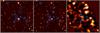 |
Fig. 1 Images of the quasar field. Left: Subaru z′ image, Middle: Spitzer Ch2, Right: Herschel PACS 100 and 160 μm images combined (pixel scale 4″). The field of view is 3 × 3 arcmin. N is up and E to the left. The five unlabelled circles are examples of sources detected in PACS. Q marks the quasar, S the nearby bright star (Spitzer photometry, Sect. 2.3), and G the nearby galaxy (PACS photometry, Sect. 2.5.1). |
Full SED of ULAS J1120+0641.
2. New observations and data reduction
The new photometric observations of ULAS J1120+0641 are summarised in Table 1. In the following sub-sections we outline the data reduction steps and how the photometry was performed. In most cases the photometric errors are dominated by sky noise, including photon (Poisson) noise and, at the longest wavelengths, confusion noise. At all wavelengths the sky noise was estimated by placing apertures on the sky and measuring the standard deviation in the histogram of sky-subtracted aperture fluxes, established from measurement of the negative wing of the Gaussian distribution. Where necessary, any gradients in the sky were removed before this step. In the case of high signal-to-noise ratio (S/N) detections, photon noise from the source was added in quadrature. For the Herschel observations we followed very similar procedures to those used by Leipski et al. (2013). All resulting photometry is presented in Table 2.
At all wavelengths longer than Spitzer Ch2 (i.e. beyond 5 μm), the measured flux is less than 2σ. We have recorded the measured flux, even if negative, and the uncertainty, rather than quote upper limits, which contain less information. This is useful when we fit models (Sect. 3), where the only free parameter is the normalisation. By fitting to the fluxes all the measurements are used simultaneously, and combine to constrain the normalisation.
2.1. Subaru
Images of the field of ULAS J1120+0641 were taken with the Suprime-Cam instrument (Miyazaki et al. 2002) on the Subaru Telescope, in the Sloan Digital Sky Survey (SDSS) i′ and z′ filters over 2011 January 9–11. Total exposure times of usable data of 150 min in i′ and 69 min in z′ were obtained, made up from individual exposures of, respectively, 180 s and 300 s. The data were reduced and combined using Version 2.0 of the SDFRED package (Ouchi et al. 2004), and the photometric calibration was applied using aperture measurements of unsaturated stars in SDSS (Ahn et al. 2014). A section of the z′ image is reproduced in Fig. 1, left.
2.2. UKIRT
The integration time of the original (discovery) UKIRT Infrared Deep Sky Survey (UKIDSS) Large Area Survey (LAS) YJHK images was 40 s (Lawrence et al. 2007). Deeper YJ photometry of the source was provided in Mortlock et al. (2011). We also obtained 500 s exposures in both H and K, on both 2011 January 24 and 26. The S/N on the later date was a factor two better than on the earlier date. These data were processed by the standard Wide-Field Camera (WFCAM) pipeline. The frames were calibrated using LAS photometry of bright stars in the field, and the data from the two nights were combined using inverse-variance weights. The measurements on the two nights were consistent with each other. The combined result of H = 18.88 ± 0.05 (Table 2) is not in agreement with the LAS survey measurement H = 18.24 ± 0.14 (from May 2008), whereas there is good agreement in Y, J, and K between both epochs. We were unable to identify any issues with the data that could explain this discrepancy. Although there is evidence that the source is variable (Page et al. 2014; Simpson et al. 2014), variability is not the explanation here, because the H and K observations were taken almost simultaneously both in the survey and in the follow up, yet the measured colour has changed significantly Δ(H − K) = 0.59 ± 0.23. The newer H value is also discrepant when compared against a model fit to all the UKIRT data (Sect. 3.2) and should therefore be considered uncertain.
2.3. Spitzer
We obtained mid-IR observations using the Spitzer InfraRed Array Camera (IRAC; Fazio et al. 2004) in Ch1 (3.6 μm) and Ch2 (4.5 μm) in July 2011. By this time Spitzer was executing the Warm Mission, so the longer wavelength channels, Ch3, Ch4, and MIPS were unavailable. Standard pipeline mosaics were downloaded from the Spitzer Heritage Archive1. A section of the Ch2 image is reproduced in Fig. 1, centre. A median filter was applied to remove a visible gradient in the sky background in both images. There is a bright star 15″ to the NW of the source, marked S in Fig. 1. Consequently, a small aperture, of radius 4″, was used for the aperture photometry. An aperture correction was applied to account for this small size as prescribed by the IRAC Instrument Handbook2.
2.4. WISE
WISE photometry of ULAS J1120+0641 from the All-Sky mid-infrared survey has been published by Blain et al. (2013). The W1 (3.4 μm) and W2 (4.6 μm) measurements listed there are superseded by our much deeper Spitzer measurements, described above. Blain et al. (2013) provide only upper limits for the W3 (12 μm) and W4 (22 μm) bands. These are quoted as the measured flux plus two times the sky noise. Since we need fluxes, rather than limits, we downloaded the ALLWISE W3 and W4 images. These images are the same as those from the All-Sky mid-infrared survey, but with improved astrometry. As with the Spitzer images a gradient in the background was removed before estimating the sky noise. The nearby star that is visible in Spitzer Ch1 and Ch2 is very faint at these wavelengths, so standard WISE apertures of radii  (W3) and
  (W4) were used. Calibration followed the procedures described in the ALLWISE Explanatory Supplement3. Our 2σ upper limits are consistent with the upper limits quoted by Blain et al. (2013).
2.5. Herschel
2.5.1. PACS
We observed the source with the Photodetector Array Camera and Spectrometer (PACS; Poglitsch et al. 2010) at 100 and 160 μm. We obtained two maps with scan angles of 70° and 110°, with data taken in miniscanmap mode using a scan speed of 20″ s-1 and a scan leg length of 4′.
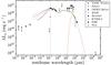 |
Fig. 2 Full SED of ULAS J1120+0641. All measurements with significance >1σ are plotted with error bars. Measurements below 1σ significance are plotted as upper limits (downwards arrows) at a value equal to 2σ (NB not measured flux+ 2σ). The mean quasar template for all SDSS quasars in Richards et al. (2006), fitted to the UKIRT and Spitzer points, is shown by the green line. The orange dashed line is a modified black body (β = 1.6 as used by Beelen et al. 2006 and defined in Sect. 3.3, T = 47 K) fitted to the 1.3 mm data point. The vertical grey line indicates the rest frame wavelength of Lyα emission. The solid magenta line in the EUV region 10-3−0.12 μm is the power-law fit from Telfer et al. (2002) for radio-quiet quasars, α = −1.57 ± 0.17, with the uncertainty indicated by the dotted lines. The i′, z′ Subaru observations are not expected to match the intrinsic SED as the continuum is strongly absorbed at these wavelengths. |
Data reduction was performed using the Herschel interactive processing environment (HIPE; Ott 2010), version 11.0.1. Maps were produced with a custom pixel scale of 1″ using Herschel Level 1 data products and the map-making routine Scanamorphos (Roussel 2013). An independent set of maps was also produced using unimap (Piazzo et al. 2012), as yet unavailable in HIPE. In both cases, the data were processed separately for the two scan directions before being mosaicked. To help in visualising the significance of the PACS measurements of the quasar, we also created an image by combining the 100 and 160 μm images, binned to 4″ pixels. This is reproduced in Fig. 1, right.
The flux of the quasar was measured in the PACS mosaics using aperture photometry within HIPE. Results were similar for both reductions, and so were averaged. The radius of the aperture was kept to 7″ to avoid a neighbouring galaxy, marked G in Fig. 1, and an appropriate aperture correction was applied (Poglitsch et al. 2010). To estimate the sky noise we measured the flux in 450 apertures of radius 7″ positioned randomly on the sky (e.g. Lutz et al. 2011; Leipski et al. 2013). The only condition on the placement of these apertures was that the central pixel should have an integration time of at least 80% of that of the quasar, established from the coverage files. We applied a small correction factor to the sky noise estimate to account for the lower average integration time of these measurements, compared to the integration time for the quasar.
2.5.2. SPIRE
We also observed ULAS J1120+0641 with the Spectral and Photometric Imaging Receiver (SPIRE; Griffin et al. 2010) at 250, 350 and 500 μm for 14 repetitions, in small scan map mode. Standard pipeline images were downloaded from the Herschel Science Data Archive4. Source extraction was performed on the maps using the built-in HIPE task sourceExtractorSussextractor (Savage & Oliver 2007), following recommendations provided in the SPIRE Observer’s Manual5. No sources were detected within 20″ of the quasar position.
Detected sources were subtracted from the SPIRE maps to leave a residual image. The residual maps were recalibrated in units of Jy/pixel using values from the SPIRE Data Reduction Guide (DRG)6. We used apertures of radius 22,32,40″ for the 250,350,500 μm wavelength images respectively. We measured small positional offsets of the SPIRE images relative to Spitzer, of a few arcsec, and corrected for these before measuring the flux at the position of the quasar. The uncertainty was then estimated in the same way as for the PACS maps. Our noise measurements are consistent with the confusion noise measurements presented by Nguyen et al. (2010).
2.6. JCMT
The source was observed with SCUBA-2 at 450 and 850 μm, at the James Clerk Maxwell Telescope (JCMT), by the instrument team in guaranteed time. The total integration time in each band was nearly 9 h, and the images reach deeper than the Herschel observations because of the deeper confusion limit, a result of the larger telescope aperture. The total observing time was split into 13 separate observations. All observations were carried out in weather bands 1 and 2 (i.e., an optical depth of τ225 GHz< 0.08). The data are of uniformly high quality, and we found no benefit in using lower weights for band 2 relative to band 1 in creating the mosaics. The raw data were downloaded from the SCUBA-2 archive7. The data were reduced using the SMURF package developed by Chapin et al. (2013) and provided by the STARLINK software project8. The raw files were processed into 13 individual maps, one per observation, using the SMURF configuration file dimmconfig_blank_field.lis. A standard flux correction factor was applied to the maps to calibrate them in mJy. They were then mosaicked using the PICARD package9. A standard matched filter was applied for the source detection.
Some of the SMURF parameters were adjusted from their default values. The most important of these is the filtering parameter filt_edge_largescale (FEL), for which the default value is 200. We experimented with values of FEL = 150, 200, 250. The noise was assessed in the usual way from the variance in apertures placed randomly in the field, within the region of high coverage. For FEL = 250, and larger values, rings appear in the final image, and a bright spot appears at the centre, giving the impression of a source. But the measured S/N is not significant, showing that the spot is an artefact that is a consequence of an incorrect choice of the value of FEL. We found that setting FEL = 150 produced the best results, as quantified by the measured S/N of two bright sources in the field. Therefore we settled on this value of FEL, which produced a flat image.
3. Analysis
The full SED of ULAS J1120+0641 is provided in Table 2, comprising the results from Sect. 2 and previously published results, from the references cited in Sect. 1. The SED is shown in Fig. 2, plotting the quantity λLλ(= νLν) against restframe wavelength, covering the range 0.2 Å−2.6 cm.
We are interested in using the SED to measure the bolometric luminosity Lbol of the source and to estimate the contributions to Lbol from the active galactic nucleus (AGN) and from star formation. Below, we measure the contribution to Lbol over the wavelength range 0.12−103 μm by fitting physically motivated models to the data. Although six of the new measurements (the two WISE, the three SPIRE, and the 450 μm SCUBA-2 values) are below 1σ, the 1σ depths reached are comparable to the expected flux levels, and so the observations provide useful constraints on the SED at these wavelengths. The contributions to Lbol at X-ray and radio wavelengths are much smaller than the uncertainties of the far-IR contribution and so may be neglected in this analysis.
Also plotted on Fig. 2 is the mean SDSS quasar template SED from Richards et al. (2006), normalised to the UKIRT and Spitzer observations. The Richards et al. (2006) template appears to provide a satisfactory fit to the Herschel and SCUBA-2 data, and there is a suggestion that the AGN could be responsible for a significant proportion of the restframe 158 μm continuum flux (observed 1.3 mm). There are, however, a number of reasons why such a conclusion would be premature. First, as emphasised by Richards et al. (2006), there is wide variation between the SEDs of quasars, so normalising the template to the restframe optical part will not necessarily provide a good fit to the far-infrared region. Second, the longest wavelength section of the template SED, beyond 50 μm restframe, falls off steeply, but the slope is not well determined. This part of the template derives from the older template of Elvis et al. (1994). To create the AGN template, the correction for host-galaxy light (i.e. star formation) at these wavelengths is substantial and uncertain.
An alternative possibility is that most of the measured flux at restframe 158 μm is from interstellar dust, heated by star formation. In order to disentangle the contributions to the SED from star formation and the AGN itself we fit models to the data, following a similar procedure to that used by Leipski et al. (2013, 2014), but with fewer free parameters, considering the low S/N of the data. We use three components to model the SED over the wavelength range 0.12−103 μm: an unobscured accretion disk and broad-line region (AD); a dusty clumpy torus (DT); and, representing the results of star formation, a modified black body (BB) of temperature 47 K. We also need to include the contribution to Lbol from the extreme ultra-violet (EUV) region, i.e., restframe wavelengths 10-3−0.12 μm. We now describe each of these components in turn.
3.1. EUV component
The spectra of quasars at extreme ultra-violet wavelengths are poorly known because much of the region is unobservable due to absorption by gas in the host galaxy and in the intervening intergalactic medium. Telfer et al. (2002) have created composite spectra over the wavelength range 0.05−0.12 μm. For radio-quiet quasars (as ULAS J1120+0641) they find α = −1.57 ± 0.17, where fν ∝ να. As shown in Fig. 2, the Telfer et al. result, extrapolated to X-ray wavelengths, lies substantially above the XMM-Newton X-ray measurements. Nevertheless, it is the slope near the peak that primarily determines the integrated luminosity. Therefore we have integrated the power-law over the wavelength range 10-3−0.12 μm, to obtain LEUV = 8.8 ± 2.2 × 1046 erg s-1 = 2.3 ± 0.6 × 10¹³ L⊙, which is adopted as the contribution to Lbol from wavelengths shortward of Lyα. Page et al. (2014) present evidence that ULAS J1120+0641 faded in X-rays between the time the source was observed by Chandra, and by XMM-Newton, so it is unclear if the X-ray points plotted represent the typical state.
Compared to the Telfer et al. (2002) spectrum, the Richards et al. (2006) template falls off more steeply and yields LEUV = 4.3 × 1046 erg s-1. The difference is likely mostly due to absorption by neutral hydrogen which was not corrected for by Richards et al. A more sophisticated treatment together with a detailed discussion is presented in Krawczyk et al. (2013).
3.2. AD component
In contrast to the EUV regime, the contribution to Lbol from restframe wavelengths between 0.12−1.0 μm is very tightly constrained by the data. For the AD component we use an updated version of the models of Maddox et al. (2012) over the wavelength range 0.12−3 μm, shown as the red line in Fig. 4, cut off as a power law at longer wavelengths as fν ∝ ν2 (Hönig & Kishimoto 2010). The photometry at H is discrepant (Sect. 2.2) and was not used in the fit. We measure LAD = 7.9 ± 0.2 × 1046 erg s-1 = 2.1 ± 0.1 × 10¹³ L⊙.
3.3. DT component
For the DT component we employ the clumpy torus models of Hönig & Kishimoto (2010). These models have several free parameters, including inclination angle, and variables characterising the dust distribution (radial and vertical scale heights, size and number of clouds). We have restricted ourselves to the 960 models with inclination angle ≤45°, consistent with a Type 1 quasar. Our fundamental assumption in using these models is that they provide a reasonable representation of the full range of SEDs of the dusty torus.
3.4. BB component
For the BB component we assume an optically thin modified black body using a dust emissivity power law index of β = 1.6. We adopt a temperature of T = 47 K (Beelen et al. 2006), which is the average temperature found by these authors in their fits to the SEDs of six high-redshift quasars, with a range 40−60 K. Since our data are not good enough to determine the temperature of the BB fit, we have taken this average value as representative. At the redshift of ULAS J1120+0641 the temperature of the CMB is TCMB = 22 K. Compared to the 47 K BB component, heating by the CMB makes a negligible contribution to the flux (da Cunha et al. 2013). On the other hand, the CMB does influence the photometry. The measured sky-subtracted flux from a blackbody source warmer than the CMB will be measured too low. For a 47 K blackbody at z = 7.084, the measured background-subtracted flux at restframe 158 μm should be multiplied by the factor 1.13 to compensate (Eq. (18), da Cunha et al. 2013). At redshift z = 6 the factor is 1.06. We have chosen not to apply any corrections to quoted 158 μm fluxes (Sect. 4) because the factors are relatively small compared to the observational errors, and because the actual blackbody temperature is unknown, meaning that the correction is quite uncertain.
3.5. Modelling the DT and BB components
To investigate the contribution of the AGN at 158 μm, we begin by fitting the DT models directly to the WISE, Herschel and SCUBA-2 fluxes, with normalisation as a free parameter, by minimising χ2 for each model. That is, the best estimate of the normalisation s for each torus model is the value that minimises 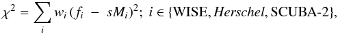 (1)where wi is the inverse variance of each observation, i.e.
  , fi is the observed flux, and Mi is the value of the model under consideration at the wavelength of the observation. It is worth reiterating that we fit the models to the fluxes from WISE, PACS, SPIRE and SCUBA-2 rather than limits, regardless of their significance. Differentiating Eq. (1) with respect to s and setting the derivative to zero yields our best estimate of the normalisation for an individual model:
 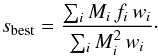 (2)The uncertainty in s, σs, is given by
  (3)For this stage our fitting procedure did not correct for any contribution of the AD and BB components over these wavelengths, which therefore maximises the DT normalisation, and therefore the contribution of the AGN at 158 μm. Since the modified black body peaks in λLλ at a restframe wavelength near 55 μm, in terms of whether we can rule out a significant contribution by the AGN at 158 μm, our approach is conservative. The results are provided in Fig. 3 where we plot the cumulative distribution of the proportion of the 158 μm continuum flux contributed by the AGN. Even though the DT normalisation has been maximised, the largest contribution at 158 μm of any of the 960 models is 53%, while 90% of the models contribute <30%. This implies that the BB component provides the dominant contribution to the 158 μm continuum flux.
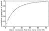 |
Fig. 3 Proportion of the 158 μm continuum flux that can be accounted for by the Hönig & Kishimoto (2010) torus models. |
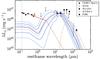 |
Fig. 4 Dusty torus model fits. The data points are the same as in Fig. 2, with the X-ray and radio ranges cropped. The red line represents the AD model, with a break to fν ∝ ν2 indicated by the red dashed line beyond 3 μm in the rest frame (Hönig & Kishimoto 2010). The AD and BB (orange line) models were subtracted from the WISE/Herschel/SCUBA-2 data, and the 960 models of Hönig & Kishimoto (2010) were fitted to the subtracted data. The solid blue lines show the median (darkest) of the fits and the 68% and 95% (lightest) ranges. The dotted blue lines represent the statistical uncertainty for an individual fit. |
Best-fit model SED.
Accordingly, we now assume that the contribution to the SED from star formation is characterised by the BB fit to the 158 μm continuum flux. Further justification for this assumption is provided in Sect. 4.1. The BB fit is shown as the dashed curve in Figs. 2 and 4. Integrating under this curve to determine the BB contribution to Lbol, we find LBB = 7.8 ± 2.0 × 1045 erg s-1 = 2.0 ± 0.5 × 10¹² L⊙ (LBB is the same as LTIR in Venemans et al. 2012). The BB fit and the AD fit described above were then subtracted from the observations, and we proceeded by refitting the clumpy torus models to the subtracted WISE/Herschel/SCUBA-2 fluxes, to estimate the DT contribution to the bolometric luminosity.
The results of the DT analysis are illustrated in Fig. 4. The spread in fitted flux at any particular wavelength, except near the PACS wavelengths, is dominated by the range of model fits, rather than by the statistical uncertainty in the normalisation of any fit. For the 960 models, we extract the median value of λLλ as well as the 68% and 95% range at each wavelength. These are plotted as solid lines in the figure. In fitting any particular torus model the uncertainty in the normalisation is typically 40%. The dashed lines plotted around the median fit illustrate this statistical uncertainty. For each model we integrate over wavelength to obtain LDT, and estimate the uncertainty in this quantity from the range over all models, combined in quadrature with the statistical uncertainty. The result is LDT = 8.4 ± 5.3 × 1046 erg s-1 = 2.2 ± 1.4 × 10¹³ L⊙, very similar to the measured value of LAD but with a much larger uncertainty. It is noticeable from Fig. 4 that the largest contribution to the uncertainty in LDT comes from the lack of constraints at restframe wavelengths in the region of 5 μm, where Spitzer 24 μm observations proved valuable for the sample of Leipski et al. (2014). Future observations with the James Webb Space Telescope will enable us to constrain LDT more tightly than the current WISE observations, with mid-infrared sensitivity over the 5−28 μm wavelength range (Gardner et al. 2006).
In Fig. 5 we show the best-fit model SED, summing the four components, and the SED is given in Table 3.
Components contributing to the bolometric luminosity.
3.6. Bolometric luminosity
Summing the contributions from the four components above, we obtain Lbol = LEUV + LAD + LDT + LBB = 2.6 ± 0.6 × 1047 erg s-1 = 6.7 ± 1.6 × 10¹³ L⊙. We tabulate the different contributions to Lbol in Table 4, expressed in erg s-1, or L⊙, and as the percentage contribution to Lbol.
We now compare the measured value of Lbol to the Eddington luminosity of the black hole. The bolometric luminosity is the total rate of flow of energy over a sphere centred on the source. The quantity Lbol, i.e. the integral under the SED, will equate to the (true) bolometric luminosity only if the emission is isotropic, which is almost certainly untrue. This point is discussed by Marconi et al. (2004) and Richards et al. (2006). Marconi et al. (2004) advocate ignoring the far-infrared contribution to Lbol, since this energy is effectively counted twice. Referring to Table 4 we see that the EUV and AD components account for 0.65Lbol. If these two components suffer from extinction, however, this sum will underestimate the true bolometric luminosity. This means that the true bolometric luminosity lies within the range 0.65−1.0Lbol. For the remainder of the paper we simply assume that the measured value of Lbol is close to the true value.
The black hole mass is ~2 × 10⁹ M⊙ (Mortlock et al. 2011; De Rosa et al. 2014). While variations in the data and analysis methods provide different formal estimates, in both cases the uncertainty is dominated by the 0.55 dex uncertainty in the normalisation of the Vestergaard & Osmer (2009) scaling relation. The Eddington ratio is hence Lbol/LEdd ≃ 1, with a comparably large relative uncertainty.
 |
Fig. 5 Best-fit model SED. Contributions from the EUV, AD, DT and BB components are all included. The curve is tabulated in Table 3. |
4. Discussion
4.1. Star formation
Modelling the SED of ULAS J1120+0641 using four components shows the BB component makes only a small contribution to Lbol, and therefore our estimate of Lbol is not sensitive to our assumption that the BB fit to the 158 μm continuum point is a good representation of the contribution of star formation to the SED. Nevertheless the issue of star formation in high-redshift quasars bears on the questions of the timescale for reaching supersolar metallicities in the broad line region, and of the origin of the correlation between black hole mass and host-galaxy bulge mass. Therefore we now consider this issue further.
In starburst galaxies most of the energy from young stars is absorbed by dust and re-emitted at far-infrared wavelengths. The best estimate for the SFR in starburst galaxies uses the relation SFR(M⊙ yr-1) = 4.5 × 10-44LTIR(erg s-1), from Kennicutt (1998), where LTIR refers to the luminosity integrated over the IR spectrum between 8−1000 μm. A far-infrared bump is ubiquitous in the SEDs of quasars, but the relative contributions from star formation or the AGN, and the luminosity dependence of this ratio is a matter of extensive debate, with no clear consensus (e.g. Haas et al. 2003; Netzer et al. 2007; Wang et al. 2011). Consequently, LTIR(8−1000 μm) only provides an upper limit to the SFR in quasars. By integrating the SED fits from the previous section over the wavelength range 8−1000 μm and applying the Kennicutt relation we obtain the distribution for the upper limit on star formation for ULAS J1120+0641, which is found to be 2700 ± 400 M⊙ yr-1.
Sargsyan et al. (2012, hereafter S12) and Sargsyan et al. (2014, hereafter S14) have investigated the use of the [C ii] 158 μm line luminosity as a measure of SFRs. From PACS spectroscopy of 130 low-redshift galaxies, including AGN, starbursts, and composites, they find that the [C ii] line strength is closely correlated with the strength of certain mid-IR line features that are indicators of star formation, particularly the PAH 11.3 μm feature and the [Ne ii] line. Furthermore, the line ratios are independent of classification into starburst or AGN. S14 conclude that the relation log [SFR /M⊙ yr-1] = log [L( [C ii] ) /L⊙] −7.0 ± 0.2 measures the SFR in an individual source. In addition S12 argue that the far-infrared luminosity LTIR is only a reliable SFR indicator in the absence of an AGN, and that the contribution from the AGN explains why the luminosity ratio L[C ii]/LTIR falls at high luminosities, LTIR> 1012 L⊙. In contrast, S14 find that the restframe 158 μm continuum luminosity L158 is correlated with the [C ii] luminosity, for AGN as well as starbursts. Therefore they argue that L158 is also a reliable SFR indicator given by the relation log [SFR /M⊙ yr-1] = log [λLλ(158 μm) / erg s-1] −42.8 ± 0.2.
Measurements of equivalent width of [Cii] for z> 5.7 quasars.
The [C ii] and 158 μm continuum SFR relations proposed by S14 are potentially important, because they apply to AGN as well as starbursts. These SFR relations are based on an analysis of low-redshift sources, nearly all at z< 0.1, and it is unclear if they hold for the high redshift and high luminosity of ULAS J1120+0641. Nevertheless if both L[C ii] and L158 are reliable SFR indicators for luminous sources, both AGN and starbursts, over a range of luminosities and redshifts, a prediction is that the ratio L[C ii]/L158, i.e. the [C ii] equivalent width (EW), should be similar for quasars at very high redshift z> 6.
S14 measure a median (restframe) [C ii] EW of 1.0 μm for low-redshift starbursts. In Table 5 we collect measurements from the literature of the [C ii] EW for eight z> 5.7 quasars. The unweighted mean EW for the eight quasars is 0.6 μm, and the inverse-variance-weighted mean is 0.5 μm. This is only a factor two smaller than the value of S14, despite the much higher 158 μm luminosities of some of the sources, and the large redshift difference. The suggestion is that the [C ii] line luminosity and restframe 158 μm continuum luminosity are promising tools for estimating the SFR in luminous high-redshift quasars, and that additional measurements over a range of redshifts and luminosities would be useful in the future.
ULAS J1120+0641 has a measured [C ii] restframe EW of 0.89 ± 0.26 μm, consistent with the predicted value of 1.0 μm, and therefore providing support for the BB fit used in the previous section. Applying the S14 SFR relations to the measurements for ULAS J1120+0641, from Venemans et al. (2012), and listed in Table 5, we find SFR[C ii] = 60−220 M⊙ yr-1 and SFR158 = 60−270 M⊙ yr-1.
4.2. The ratio MBH/Mbulge
We now consider the relationship between the mass of the central black hole in galaxies, MBH, and the stellar mass of the bulge, Mbulge. An analysis by Häring & Rix (2004) of 30 nearby galaxies yielded a tight relation between the two quantities. The relation is almost linear, with a fiducial ratio MBH/Mbulge ≃ 1.4 × 10⁻³. If we equate the quasar SFR to the rate of increase of the bulge stellar mass, Ṁbulge, we are interested in computing the rate of increase of the black hole mass, ṀBH, and comparing the ratio of the growth rates to the mass ratio observed in galaxies today. In other words, at the time observed, is the black hole or the bulge growing faster relative to the mass ratio measured in the local universe?
The luminosity of a black hole is given by Lbol = ηṀc2, where η is the black hole efficiency and Ṁ is the accretion rate. We consider mass that is not converted to energy through accretion as contributing to the increase of the black hole mass, i.e.,  . From our value of Lbol = 2.6 × 1047 erg s-1, and assuming an efficiency η = 0.1, we estimate ṀBH = 40 M⊙ yr-1. Adopting a SFR of ~200 M⊙ yr-1, we find ṀBH/Ṁbulge ≃ 40 M⊙ yr-1/200 M⊙ yr-1 = 0.2. Comparing this quantity to the local mass ratio MBH/Mbulge ≃ 1.4 × 10⁻³, the black hole was growing in mass more than 100 times faster than the stellar bulge, relative to the mass ratio measured in the local universe.
5. Summary
Combining published measurements and new observations, we have compiled a full multi-wavelength SED for the z = 7.1 quasar ULAS J1120+0641, summarised in Table 2, and plotted in Fig. 2. In particular, the SED included new observations in the far-infrared and sub-mm.
We now summarise the main results of the paper.
-
1.
Based on an analysis that used the dusty torus models of Hönig & Kishimoto (2010), we find that the torus does not contribute a significant fraction of the restframe 158 μm continuum flux, which we ascribe instead to star formation.
-
2.
From the model fits we measure a bolometric luminosity of Lbol = 2.6 ± 0.6 × 1047 erg s-1 = 6.7 ± 1.6 × 10¹³ L⊙, where the main source of uncertainty is the lack of deep observations at ~40 μm, corresponding to 5 μm in the rest frame of the quasar.
-
3.
A comparison of the [C ii] EWs in a sample of z> 5.7 quasars with the measured values for starburst galaxies in the local universe suggests that the [C ii] line luminosity and restframe 158 μm continuum luminosity are promising indicators for estimating the SFR in luminous high-redshift quasars.
-
4.
Based on the [C ii] luminosity and the restframe 158 μm continuum luminosity we estimate a SFR in ULAS J1120+0641 of 60−270 M⊙ yr-1.
-
5.
We find that, at the time observed, the black hole was growing in mass more than 100 times faster than the stellar bulge, relative to the mass ratio measured in the local universe.
Acknowledgments
We are grateful to Cristian Leipski for correspondence on PACS and SPIRE data reduction and photometry, to Bruno Altieri who produced the unimap PACS image, to Ros Hopwood for additional expert advice on the Herschel data, to Jim Geach for advice on processing the SCUBA-2 data, and to Tom Kerr for much help through the UKIRT service programme. S.W. gratefully acknowledges the support of the Leverhulme Trust through the award of a Leverhulme Research Fellowship. B.P.V. acknowledges funding through the ERC grant “Cosmic Dawn”. Based in part on data collected at Subaru Telescope, which is operated by the National Astronomical Observatory of Japan. The United Kingdom Infrared Telescope was operated by the Joint Astronomy Centre on behalf of the Science and Technology Facilities Council of the UK. Some of the data reported here were obtained as part of the UKIRT Service Programme. This work is based in part on observations made with the Spitzer Space Telescope, which is operated by the Jet Propulsion Laboratory, California Institute of Technology under a contract with NASA. This publication makes use of data products from the Wide-field Infrared Survey Explorer, which is a joint project of the University of California, Los Angeles, and the Jet Propulsion Laboratory/California Institute of Technology, funded by the National Aeronautics and Space Administration. Herschel is an ESA space observatory with science instruments provided by European-led Principal Investigator consortia and with important participation from NASA. The James Clerk Maxwell Telescope has historically been operated by the Joint Astronomy Centre on behalf of the Science and Technology Facilities Council of the United Kingdom, the National Research Council of Canada and the Netherlands Organisation for Scientific Research. Additional funds for the construction of SCUBA-2 were provided by the Canada Foundation for Innovation.
References
- Ahn, C. P., Alexandroff, R., Allen de Prieto, C., et al. 2014, ApJS, 211, 17 [NASA ADS] [CrossRef] [Google Scholar]
- Beelen, A., Cox, P., Benford, D. J., et al. 2006, ApJ, 642, 694 [NASA ADS] [CrossRef] [Google Scholar]
- Begelman, M. C., Volonteri, M., & Rees, M. J. 2006, MNRAS, 370, 289 [NASA ADS] [CrossRef] [Google Scholar]
- Blain, A. W., Assef, R., Stern, D., et al. 2013, ApJ, 778, 113 [NASA ADS] [CrossRef] [Google Scholar]
- Bolton, J. S., Haehnelt, M. G., Warren, S. J., et al. 2011, MNRAS, 416, L70 [NASA ADS] [CrossRef] [Google Scholar]
- Bouwens, R. J., Illingworth, G. D., Oesch, P. A., et al. 2011, ApJ, 737, 90 [NASA ADS] [CrossRef] [Google Scholar]
- Chapin, E. L., Berry, D. S., Gibb, A. G., et al. 2013, MNRAS, 430, 2545 [NASA ADS] [CrossRef] [Google Scholar]
- Croom, S. M., Smith, R. J., Boyle, B. J., et al. 2004, MNRAS, 349, 1397 [NASA ADS] [CrossRef] [Google Scholar]
- da Cunha, E., Groves, B., Walter, F., et al. 2013, ApJ, 766, 13 [Google Scholar]
- De Rosa, G., Venemans, B. P., Decarli, R., et al. 2014, ApJ, 790, 145 [NASA ADS] [CrossRef] [Google Scholar]
- Dietrich, M., Hamann, F., Appenzeller, I., & Vestergaard, M. 2003a, ApJ, 596, 817 [NASA ADS] [CrossRef] [Google Scholar]
- Dietrich, M., Hamann, F., Shields, J. C., et al. 2003b, ApJ, 589, 722 [NASA ADS] [CrossRef] [Google Scholar]
- Elvis, M., Wilkes, B. J., McDowell, J. C., et al. 1994, ApJS, 95, 1 [NASA ADS] [CrossRef] [Google Scholar]
- Fan, X., Strauss, M. A., Schneider, D. P., et al. 2001, AJ, 121, 54 [NASA ADS] [CrossRef] [Google Scholar]
- Fan, X., Hennawi, J. F., Richards, G. T., et al. 2004, AJ, 128, 515 [NASA ADS] [CrossRef] [Google Scholar]
- Fan, X., Strauss, M. A., Becker, R. H., et al. 2006, AJ, 132, 117 [NASA ADS] [CrossRef] [EDP Sciences] [Google Scholar]
- Fazio, G. G., Hora, J. L., Allen, L. E., et al. 2004, ApJS, 154, 10 [NASA ADS] [CrossRef] [Google Scholar]
- Ferrarese, L., & Merritt, D. 2000, ApJ, 539, L9 [NASA ADS] [CrossRef] [Google Scholar]
- Gardner, J. P., Mather, J. C., Clampin, M., et al. 2006, Space Sci. Rev., 123, 485 [NASA ADS] [CrossRef] [Google Scholar]
- Griffin, M. J., Abergel, A., Abreu, A., et al. 2010, A&A, 518, L3 [Google Scholar]
- Haas, M., Klaas, U., Müller, S. A. H., et al. 2003, A&A, 402, 87 [NASA ADS] [CrossRef] [EDP Sciences] [Google Scholar]
- Häring, N., & Rix, H.-W. 2004, ApJ, 604, L89 [NASA ADS] [CrossRef] [Google Scholar]
- Holland, W. S., Bintley, D., Chapin, E. L., et al. 2013, MNRAS, 430, 2513 [NASA ADS] [CrossRef] [Google Scholar]
- Hönig, S. F., & Kishimoto, M. 2010, A&A, 523, A27 [NASA ADS] [CrossRef] [EDP Sciences] [Google Scholar]
- Hopkins, A. M., & Beacom, J. F. 2006, ApJ, 651, 142 [NASA ADS] [CrossRef] [MathSciNet] [Google Scholar]
- Jiang, L., Fan, X., Bian, F., et al. 2009, AJ, 138, 305 [NASA ADS] [CrossRef] [Google Scholar]
- Kauffmann, G., & Haehnelt, M. 2000, MNRAS, 311, 576 [NASA ADS] [CrossRef] [Google Scholar]
- Kennicutt, R. C. 1998, ARA&A, 36, 189 [Google Scholar]
- Krawczyk, C. M., Richards, G. T., Mehta, S. S., et al. 2013, ApJS, 206, 4 [NASA ADS] [CrossRef] [Google Scholar]
- Lawrence, A., Warren, S. J., Almaini, O., et al. 2007, MNRAS, 379, 1599 [NASA ADS] [CrossRef] [MathSciNet] [Google Scholar]
- Leipski, C., Meisenheimer, K., Walter, F., et al. 2013, ApJ, 772, 103 [NASA ADS] [CrossRef] [Google Scholar]
- Leipski, C., Meisenheimer, K., Walter, F., et al. 2014, ApJ, 785, 154 [NASA ADS] [CrossRef] [Google Scholar]
- Loeb, A., & Rasio, F. A. 1994, ApJ, 432, 52 [NASA ADS] [CrossRef] [Google Scholar]
- Lutz, D., Poglitsch, A., Altieri, B., et al. 2011, A&A, 532, A90 [NASA ADS] [CrossRef] [EDP Sciences] [Google Scholar]
- Maddox, N., Hewett, P. C., Péroux, C., Nestor, D. B., & Wisotzki, L. 2012, MNRAS, 424, 2876 [NASA ADS] [CrossRef] [Google Scholar]
- Magorrian, J., Tremaine, S., Richstone, D., et al. 1998, AJ, 115, 2285 [NASA ADS] [CrossRef] [Google Scholar]
- Marconi, A., Risaliti, G., Gilli, R., et al. 2004, MNRAS, 351, 169 [NASA ADS] [CrossRef] [Google Scholar]
- McGreer, I. D., Jiang, L., Fan, X., et al. 2013, ApJ, 768, 105 [NASA ADS] [CrossRef] [Google Scholar]
- Miyazaki, S., Komiyama, Y., Sekiguchi, M., et al. 2002, PASJ, 54, 833 [NASA ADS] [CrossRef] [Google Scholar]
- Momjian, E., Carilli, C. L., Walter, F., & Venemans, B. 2014, AJ, 147, 6 [NASA ADS] [CrossRef] [Google Scholar]
- Moretti, A., Ballo, L., Braito, V., et al. 2014, A&A, 563, A46 [NASA ADS] [CrossRef] [EDP Sciences] [Google Scholar]
- Mortlock, D. J., Warren, S. J., Venemans, B. P., et al. 2011, Nature, 474, 616 [NASA ADS] [CrossRef] [PubMed] [Google Scholar]
- Natarajan, P. 2014, Gen. Rel. Grav., 46, 1702 [NASA ADS] [CrossRef] [Google Scholar]
- Netzer, H., Lutz, D., Schweitzer, M., et al. 2007, ApJ, 666, 806 [NASA ADS] [CrossRef] [Google Scholar]
- Nguyen, H. T., Schulz, B., Levenson, L., et al. 2010, A&A, 518, L5 [NASA ADS] [CrossRef] [EDP Sciences] [Google Scholar]
- Ott, S. 2010, in Astronomical Data Analysis Software and Systems XIX, eds. Y. Mizumoto, K.-I. Morita, & M. Ohishi, ASP Conf. Ser., 434, 139 [Google Scholar]
- Ouchi, M., Shimasaku, K., Okamura, S., et al. 2004, ApJ, 611, 660 [NASA ADS] [CrossRef] [Google Scholar]
- Page, M. J., Simpson, C., Mortlock, D. J., et al. 2014, MNRAS, 440, L91 [NASA ADS] [CrossRef] [Google Scholar]
- Piazzo, L., Ikhenaode, D., Natoli, P., et al. 2012, IEEE Trans. on Image Processing, 21, 3687 [Google Scholar]
- Pilbratt, G. L., Riedinger, J. R., Passvogel, T., et al. 2010, A&A, 518, L1 [CrossRef] [EDP Sciences] [Google Scholar]
- Poglitsch, A., Waelkens, C., Geis, N., et al. 2010, A&A, 518, L2 [NASA ADS] [CrossRef] [EDP Sciences] [Google Scholar]
- Regan, J. A., & Haehnelt, M. G. 2009, MNRAS, 396, 343 [NASA ADS] [CrossRef] [Google Scholar]
- Richards, G. T., Lacy, M., Storrie-Lombardi, L. J., et al. 2006, ApJS, 166, 470 [NASA ADS] [CrossRef] [Google Scholar]
- Roussel, H. 2013, PASP, 125, 1126 [Google Scholar]
- Sargsyan, L., Lebouteiller, V., Weedman, D., et al. 2012, ApJ, 755, 171 [NASA ADS] [CrossRef] [Google Scholar]
- Sargsyan, L., Samsonyan, A., Lebouteiller, V., et al. 2014, ApJ, 790, 15 [NASA ADS] [CrossRef] [Google Scholar]
- Savage, R. S., & Oliver, S. 2007, ApJ, 661, 1339 [NASA ADS] [CrossRef] [Google Scholar]
- Simpson, C., Mortlock, D., Warren, S., et al. 2014, MNRAS, 442, 3454 [NASA ADS] [CrossRef] [Google Scholar]
- Telfer, R. C., Zheng, W., Kriss, G. A., & Davidsen, A. F. 2002, ApJ, 565, 773 [NASA ADS] [CrossRef] [Google Scholar]
- Venemans, B. P., McMahon, R. G., Walter, F., et al. 2012, ApJ, 751, L25 [Google Scholar]
- Venemans, B. P., Findlay, J. R., Sutherland, W. J., et al. 2013, ApJ, 779, 24 [NASA ADS] [CrossRef] [Google Scholar]
- Venkatesan, A., Schneider, R., & Ferrara, A. 2004, MNRAS, 349, L43 [NASA ADS] [CrossRef] [Google Scholar]
- Vestergaard, M., & Osmer, P. S. 2009, ApJ, 699, 800 [Google Scholar]
- Volonteri, M. 2010, A&ARv, 18, 279 [NASA ADS] [CrossRef] [Google Scholar]
- Walter, F., Riechers, D., Cox, P., et al. 2009, Nature, 457, 699 [NASA ADS] [CrossRef] [PubMed] [Google Scholar]
- Wang, R., Wagg, J., Carilli, C. L., et al. 2011, AJ, 142, 101 [NASA ADS] [CrossRef] [Google Scholar]
- Wang, R., Wagg, J., Carilli, C. L., et al. 2013, ApJ, 773, 44 [NASA ADS] [CrossRef] [Google Scholar]
- Willott, C. J., McLure, R. J., & Jarvis, M. J. 2003, ApJ, 587, L15 [NASA ADS] [CrossRef] [Google Scholar]
- Willott, C. J., Delorme, P., Reylé, C., et al. 2010, AJ, 139, 906 [NASA ADS] [CrossRef] [Google Scholar]
- Willott, C. J., Omont, A., & Bergeron, J. 2013, ApJ, 770, 13 [NASA ADS] [CrossRef] [Google Scholar]
All Tables
All Figures
|
Fig. 1 Images of the quasar field. Left: Subaru z′ image, Middle: Spitzer Ch2, Right: Herschel PACS 100 and 160 μm images combined (pixel scale 4″). The field of view is 3 × 3 arcmin. N is up and E to the left. The five unlabelled circles are examples of sources detected in PACS. Q marks the quasar, S the nearby bright star (Spitzer photometry, Sect. 2.3), and G the nearby galaxy (PACS photometry, Sect. 2.5.1). |
| In the text | |
|
Fig. 2 Full SED of ULAS J1120+0641. All measurements with significance >1σ are plotted with error bars. Measurements below 1σ significance are plotted as upper limits (downwards arrows) at a value equal to 2σ (NB not measured flux+ 2σ). The mean quasar template for all SDSS quasars in Richards et al. (2006), fitted to the UKIRT and Spitzer points, is shown by the green line. The orange dashed line is a modified black body (β = 1.6 as used by Beelen et al. 2006 and defined in Sect. 3.3, T = 47 K) fitted to the 1.3 mm data point. The vertical grey line indicates the rest frame wavelength of Lyα emission. The solid magenta line in the EUV region 10-3−0.12 μm is the power-law fit from Telfer et al. (2002) for radio-quiet quasars, α = −1.57 ± 0.17, with the uncertainty indicated by the dotted lines. The i′, z′ Subaru observations are not expected to match the intrinsic SED as the continuum is strongly absorbed at these wavelengths. |
| In the text | |
|
Fig. 3 Proportion of the 158 μm continuum flux that can be accounted for by the Hönig & Kishimoto (2010) torus models. |
| In the text | |
|
Fig. 4 Dusty torus model fits. The data points are the same as in Fig. 2, with the X-ray and radio ranges cropped. The red line represents the AD model, with a break to fν ∝ ν2 indicated by the red dashed line beyond 3 μm in the rest frame (Hönig & Kishimoto 2010). The AD and BB (orange line) models were subtracted from the WISE/Herschel/SCUBA-2 data, and the 960 models of Hönig & Kishimoto (2010) were fitted to the subtracted data. The solid blue lines show the median (darkest) of the fits and the 68% and 95% (lightest) ranges. The dotted blue lines represent the statistical uncertainty for an individual fit. |
| In the text | |
|
Fig. 5 Best-fit model SED. Contributions from the EUV, AD, DT and BB components are all included. The curve is tabulated in Table 3. |
| In the text | |
Current usage metrics show cumulative count of Article Views (full-text article views including HTML views, PDF and ePub downloads, according to the available data) and Abstracts Views on Vision4Press platform.
Data correspond to usage on the plateform after 2015. The current usage metrics is available 48-96 hours after online publication and is updated daily on week days.
Initial download of the metrics may take a while.