| Issue |
A&A
Volume 575, March 2015
|
|
|---|---|---|
| Article Number | A101 | |
| Number of page(s) | 8 | |
| Section | Stellar structure and evolution | |
| DOI | https://doi.org/10.1051/0004-6361/201424280 | |
| Published online | 04 March 2015 | |
V342 Andromedae B is an eccentric-orbit eclipsing binary⋆
1 Astronomical Observatory Institute, Faculty of Physics, A. Mickiewicz University, Słoneczna 36, 60-286 Poznań, Poland
e-mail: This email address is being protected from spambots. You need JavaScript enabled to view it.
2 Thüringer Landessternwarte Tautenburg, Sternwarte 5, 07778 Tautenburg, Germany
3 Nicolaus Copernicus Astronomical Center, Polish Academy of Sciences, Bartycka 18, 00-716 Warszawa, Poland
Received: 26 May 2014
Accepted: 24 January 2015
Abstract
We present a photometric and spectroscopic study of the visual binary V342 Andromedae. Visual components of the system have angular separations of 3 arcseconds. We obtained two spectroscopic data sets. An examination of both the A and B component spectra reveals that the B component is a spectroscopic binary with an eccentric orbit. The orbital period, taken from the Hipparcos Catalog, agrees with the orbital period of the B component measured spectroscopically. We also collected a new set of photometric measurements. The argument of periastron is close to 270° and the orbit eccentricity is not seen in our photometric data. About five years after the first spectroscopic observations, a new set of spectroscopic data was obtained. We analysed the apsidal motion, but we did not find any significant changes in the orbital orientation. A Wilson-Devinney model was calculated based on the photometric and the radial velocity curves. The result shows two very similar stars with masses M1 = 1.27 ± 0.01 M⊙, M2 = 1.28 ± 0.01 M⊙, respectively. The radii are R1 = 1.21 ± 0.01 R⊙, R2 = 1.25 ± 0.01 R⊙, respectively. Radial velocity measurements of component A, the most luminous star in the system, reveal no significant periodic variations. We calculated the time of the eclipsing binary orbit’s circularization, which is about two orders of magnitude shorter than the estimated age of the system. The discrepancies in the age estimation can be explained by the Kozai effect induced by the visual component A. The atmospheric parameters and the chemical abundances for the eclipsing pair, as well as the LSD profiles for both visual components, were calculated from two high-resolution, well-exposed spectra obtained on the 2-m class telescope.
Key words: binaries: close / binaries: eclipsing / stars: individual: V342 Andromedae B
Based on spectroscopy obtained at the David Dunlap Observatory, University of Toronto, Canada, Poznań Spectroscopic Telescope 1, Poland and Thüringer Landessternwarte, Tautenburg, Germany.
© ESO, 2015
1. Introduction
The majority of the field stars, about 60−80%, are binary or multiple systems (Duquennoy & Mayor, 1991). Triple stars, like V342 Andromedae, are about 17% of the non-single stars. The statistics of multiple stars give some constraints on stellar formation, which is still subject of a study that is providing new results (Zinnecker & Mathieu, 2001). The newer statistics of stellar multiplicity are presented by Raghavan et al. (2010). They found that 8% of the 454 star sample are triple stars. The existence of an eclipsing pair in multiple stellar systems provides a unique possibility for a precise determination of stellar parameters. Our observations show that the weaker component B of the visual binary V342 Andromedae is an eclipsing binary with an eccentric orbit. The presence of the third body (component A) near the eclipsing pair could cause an apsidal motion. The dynamical evolution of the triple systems was described by Harrington (1968); Mazeh & Shaham (1979). The interaction between a close binary and the farther tertiary component and resulting period changes was discussed by Pribulla & Rucinski (2006); Tokovinin et al. (2006). They investigate 151 contact binaries and 165 spectroscopic binaries. The authors discussed the Kozai cycles with tidal friction mechanism (KZTF; Eggleton & Kiseleva-Eggleton 2001) as causing the shrinking of a close pair’s orbit or a loss of the angular momentum, as well as the mechanism analogical to the so-called planet migration. The existing statistics of stellar multiplicity could be compared with the results of numerical simulations of multiple star formation (Machida et al., 2008). Simulations show that 100% of the stars at their birth are either binary or multiple. Multiple systems with an eclipsing component were catalogued by Chambliss (1992). He mentions 80 systems, but now we know more than 130. Multiples with known visual orbits were described by Zasche et al. (2009).
The multiple star V342 Andromedae is listed in the Henry Draper catalog as an A3 spectral type star. The two visual components were noted as HD 556 A and B. The Durchmusterung identification of the star is BD+45 16 and the equatorial coordinates of the system are  and δ = + 46°23′25″ (FK5). The color index of the whole system (A and B components together) B − V = 0.16 ± 0.02, is listed in the Tycho catalog, and its value corresponds to the temperature of 8140 K (Sp ≃ A5). The Morgan-Keenan (MK) spectral classification A4V was given by Abt (1981). The star was observed by Hipparcos satellite (HIC 817), and the obtained light curve revealed the variation with a period of
  and an amplitude of 0.1 mag. Also, the trigonometric parallax was measured with the value of 7.21 ± 1.55 mas. The new reduction of the Hipparcos data (van Leeuwen, 2007) provided a new value for the trigonometric parallax of 6.68 ± 1.05 mas. The star is listed among the visual binaries in CCDM Catalogue (Dommanget & Nys, 1994); the visual components have brightness of 8.1 and 9.1 V mag and are separated by 5 arcsec. Additionally, the position angle is 84°. In Table 1 we list more measurements of V342 Andromedae, the earliest and the most up-to-date values come from the Washington Double Star Catalog (Mason et al., 2001). The results for the angular separation have large differences. The WDC data present significantly lower values than other sources.
The main aim of this study is to determine the nature of the system and to identify which visual component is an eclipsing binary. There are no radial velocity curves for this star in the literature and we started a spectroscopic campaign that enabled us to obtain a model of the system. We obtained spectra with three instruments and additionally we collected a new light curve, which complements the Hipparcos photometric data.
Position angle and separation measurements from WDC and CCDM catalogs, Heintz (1967) and Alzner (1998).
2. Data
2.1. Spectroscopy
The first spectroscopic data were obtained at the David Dunlap Observatory (DDO) with 1.88 m telescope equipped with the Cassegrain spectrograph. We were unable to determine the eclipsing component. Nevertheless, based on the position angle we placed both components (A and B) on the slit. We obtained two parallel spectra with a dispersion of 0.15 Å/pix; these are presented in Fig. 1. In total, we collected 22 spectra with the exposure times of 1200 s each. The spectral range is about 300 Å near MgI triplet at wavelength 5175 Å. The typical signal-to-noise ratio is ~ 130 for the visual component A and ~ 40 for B. Main component was better positioned on the slit, since it was our primary target at the beginning of the observational campaign.
We obtained the second spectroscopic data set with the 0.5 m Poznań Spectroscopic Telescope 1 (PST1), which had already used been to observe other multiple stars with eclipsing component; in particular: DY Lyncis (Sekalska et al., 2010) and HD 86222 (Dimitrov et al., 2014). Despite the small diameter of the telescope, new components were detected in both cases. We obtained 63 echelle spectra of V342 And with exposure times of 1200 s and spectral range 4290−7520 Å (Fig. 2). The spectra are typical for a hot star, dominated by hydrogen and magnesium triplet lines. The signal-to-noise ratio in most of the spectra ranges from 40 to 50. The short focal length and poor seeing caused that both A and B components were on the fiber entrance. That is why we obtained triple-lined spectra with PST1.
Radial velocities (DDO) of the eclipsing pair V342 Andromedae B.
Data reduction and PST1 radial velocity measurements (cross correlation, FXCOR task) were provided by IRAF1 package tasks. For radial velocity measurements of DDO spectra we used the broadening function method (Rucinski, 1992, 2002). The procedure of the cosmic ray removal for PST1 spectra was made with DCR code (Pych, 2004).
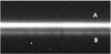 |
Fig. 1 Part of DDO spectrum, the plot shows two parallel spectra. Both visual components A and B are pointed on the slit. |
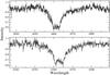 |
Fig. 2 One of the well-exposed PST1 spectra with dissociated lines (HJD = 2 455 874.243). The hydrogen Hα and Hβ lines are plotted. |
2.2. Photometry
The first photometric curve of V342 And was obtained by the Hipparcos satellite. The 164 data points were collected from 21 December 1989 to 26 January 1993 and the eclipses with similar depth were registered. Based on this curve, we suggest that the eclipsing pair has a circular orbit and the primary and the secondary eclipse are separated in phase about 0.5.
We collected our data set with the 20cm Newtonian telescope, equipped with a ST7 CCD camera in 2007 (8th August–27th November). We obtained 13282 measurements in R filter with exposure times of 5 and 20 s. The data reduction and aperture photometry were done with the Starlink package2.
In both data sets the visual components A and B were not resolved. Therefore the light curves of the eclipsing binary contain strong third light higher than 50%. Taking both Hipparcos and our datasets into account, we derived the following ephemeris:  (1)
(1)
3. Model of the system
3.1. The eclipsing pair
Spectra from DDO reveals that the weaker component B is a spectroscopic binary. The orbital period is in agreement with the photometric one. For modeling, we used original Hipparcos data and 1745 bins of our photometry. We bin our data to speed up calculations. The bin size is 0.002 day. Every bin contains from 2 to 10 points (different exposure times) for which we used a median. The dispersion of data are σHp = 0.01 and σR = 0.006 mag (after binning). Because of the specific orbital orientation, ω ~ 273° (close to  rad), the eccentricity of the orbit is not detectable in the photometry (Fig. 3). Nevertheless, the spectroscopic curves show eccentricity of about 0.08. Amplitudes of RV curves are almost equal, as presented in Fig. 4. The dispersion of the DDO radial velocity data is σRV = 1.07 km s-1. We used only DDO measurements for this model because of small systematic differences in the PST1 data (see Sect. 3.2). Both RV sets are compared in Table 5. The R light curve shows flat maxima and eclipses with similar depth and amplitude of ~0.15 mag. For modeling we used Wilson-Devinney method (Wilson & Devinney, 1971) and PHOEBE code (Prša & Zwitter, 2005). We treated the visual component A of the system as a constant third light. Temperature T1 of the main (hotter) component of V342 And B was fixed to the value of a star with the same mass and radius from the evolutionary models (Sect. 3.4). The temperature of the secondary component of the eclipsing pair was fitted during the modeling process. We used logarithmic law for limb darkening and Van Hamme (1993) coefficients. For albedo and gravity brightening coefficients, we applied values for the convective envelope of 0.5 and 0.32, respectively. Also, we assumed synchronous rotation of the components based on the estimation of the time of synchronization and age of the system (Sect. 3.4). Additionally, the new results reveal that rotation periods are equal within errors with the orbital period of the pair (Sect. 4). The result of the modeling shows two very similar main-sequence stars (Table 3). For better estimation of the parameter errors, we used a Monte Carlo (MC) simulation. We generate ten sets of synthetic LC/RV data with the same dispersion as the observations used in the modeling process. Fitting this synthetic data we obtained ten values for each parameter. As a MC error, listed in Table 3, we used a 1σ dispersion of these values. In most cases, the MC errors are comparable with the formal errors.
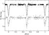 |
Fig. 3 Photometric data from our (top) and Hipparcos observations (bottom). The synthetic curves come from the fitted model. Hipparcos plot is shifted up by 0.1 mag. |
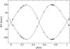 |
Fig. 4 Radial velocity curve for V342 Andromedae B, the eclipsing pair. Open circles correspond to the DDO observations measured with the broadening function method. |
Parameters of the eclipsing pair V342 Andromedae B obtained with Wilson-Devinney method.
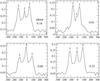 |
Fig. 5 Four examples of cross-correlation function (PST1 spectra). The three peaks are marked, the central one is connected with the main visual component A. Outer peaks correspond to component B, the eclipsing pair. Horizontal axis shows the observed velocity and vertical axis the correlation coefficient. |
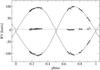 |
Fig. 6 Radial velocity curves for all three components from PST1 triple-lined spectra. Dashed horizontal line presents the mean value of the third body (visual component A) radial velocity. |
3.2. New spectroscopic data from PST1
About five years after our first spectroscopic observation at DDO, we started a new campaign with the 0.5 m telescope (PST13) equipped with the echelle spectrograph. We used a different instrument and radial velocity measurement technique (Fig. 5). The four examples of cross-correlation function are plotted. The relative height of A and B components’ peaks is changing during the night. This effect is the result of the guiding on 50 μ fiber entrance. Because of the focal length of the telescope, we could not resolve both components. If the guiding were in slightly different positions close to the photocentrum, we would have collected more light from either the A or B component. The dispersion of the PST1 measurements is σRV = 1.27 km s-1 (Fig. 6). In Table 4 the RV measurements are listed. For this data set we fitted only orbital parameters. The results are listed in Table 5. Subsequently, we compared the results with the earlier DDO set. The existence of a third body could cause apsidal motion in the orbit of the eclipsing pair, but we have not found any significant change in the argument of periastron in the five-year period between DDO and PST1 observations.
Radial velocity measurements of triple-lined PST1 spectra of V342 Andromedae.
We obtained two spectroscopic data sets, which are completely independent of each other, collected with different instruments and measured using different techniques. We decided to analyse both sets separately because of slight systematic differences in the results. For example, the calculated semimajor axis differs by about 3% for both data sets. Moreover, the Monte Carlo simulation error for DDO data is about 0.3% for the semimajor axis. The differences between the sets are caused mainly by the fact that DDO spectra are double-lined and A/B components are resolved. In case of the PST1, spectra are triple-lined because of the shorter focal length. The blending effect observed in spectral lines is stronger for the triple-lined spectrum and the measurements are less precise. The effective focal length for 1.88 m DDO telescope is 32.5 m and only 2.25 m for the PST1. Also, the surface of the PST1 main mirror is 14 times smaller than at DDO. Despite the fact that we obtain fewer photons with PST1, the adjustment of the telescope, fiber parameters, and spectrograph design results in very small light losses in the system. Additionally, the spectral range is about ten times longer, which enabled us to obtain comparable results in RV measurements to the bigger DDO telescope.
Results of fitting only the spectroscopic data from DDO and PST1 and the formal errors.
3.3. The third component
Photometric observations show that component A is the most luminous star in this triple system. We treated this component in the Wilson-Devinney model as a constant third light. The color of the system corresponds to about A5 spectral type. The mass and radii of the eclipsing pair components correspond to a lower temperature and spectral type of about F7. Because of the mixing of the light, the temperature of the third body (visual A component) must be higher than the temperature corresponding to the color temperature of the whole system (TA> 8140 K). The radial velocities of the third component (Table 4) show some variation but we did not find any significant periodicities. For the analysis, we used the G. Maciejewski code based on the Schwarzenberg-Czerny (1996) method. The mean value of the radial velocity of the third component is 3.5 ± 2.2 km s-1, which is 8.0 km s-1 higher than the velocity of the center of mass of the eclipsing pair. The new results (Sect. 4) show that component A could also be binary and the measured peak (RV3) corresponds to the sharp-lined component of V342 Andromedae A (Fig. 8).
3.4. Distance and age of the system
We calculated the distance of V342 And using the photometric parallax method and values from the WD model. The result, 142 ± 9 pc, is in good agreement with the Hipparcos measurements (150 ± 20 pc), from which it differs by about 5%.
We list the values of position angle and separation of the visual components A and B of V342 Andromedae in Table 1. One can see a poor agreement between the catalogs. With the values from the Washington Double Star Catalog, we made a very rough estimation of the orbital period (visual A and B orbit) and a separation of the components taking the distance of the system into account. The period is about 2 × 10⁴ years and the separation is about 464 AU.
We suggest, based on masses and radii, that the eclipsing pair components are main-sequence stars. Figure 7 presents the Yonsei-Yale4 evolutionary tracks and both components are plotted (Yi et al., 2001, 2003; Kim et al., 2002). The age of the system for these values of mass and radii is between 2 and 3 Gyr. The component with higher mass has lower temperature. It is typical for pairs of very similar stars in which the more massive component overtakes the less massive on the evolutionary track. In this case, the temperature of the secondary component is too low, fitting about 170 K lower than the evolutionary model suggests. The time of circularization of the eclipsing binary orbit is about 4 × 10⁷ yr, according to an equation given by Zahn (1975). It is significantly shorter than the estimated age of the system. The explanation of this fact could be the existence of a massive third body, visual component A, which could excite Kozai (1962) cycles. The time of synchronization, calculated with the equation given by Zahn (1977), is about 5 × 10⁵ years for both components.
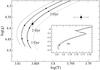 |
Fig. 7 Evolutionary tracks for both components of the eclipsing pair V342 And B. Solid lines present the tracks and dotted and dashed lines their error bars. The subframe shows the same curves zoomed out. Component 1 lays on its track and component 2 is shifted toward lower temperatures. |
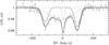 |
Fig. 8 Best fit (thick continuous line) of the LSD profile (thin) from one PST1 spectrum and the underlying double-Gaussian profiles for components A (dotted) and B (dashed). |
4. Spectrum analysis
We used the least squares deconvolution (LSD) technique (Donati et al., 1997) to reveal the basic shapes of the line profiles of stars A and B in our composite PST1 spectra. It can be seen from Fig. 8 that the profile of star A can only be fitted when assuming a broad plus a sharp component. This is confirmed by one spectrum of component A taken with the Coude-Echelle spectrograph of the Thüringer Landessternwarte (TLS) Tautenburg in December 2014 with a resolving power of 58 000 (top of Fig. 9). The inspection of our time series of PST1 spectra and the comparison with the TLS spectrum shows that the sharp-lined component is stationary in radial velocity. We assume that star A is a SB2 star. The epoch difference between the PST1 and the TLS observations is more than three years. Thus, if component A is a physical binary, its orbital period must be of the order of decades or longer.
In a first attempt, we tried to decompose the PST1 spectra into components A and B by applying the KOREL program (Hadrava, 1995) to our time series, and using the model of an artificial hierarchical system consisting of the close binary star B plus star A in a wide orbit. The results showed, however, that we could not reproduce the extraordinary shape of the line profiles of star A. We assume that the decomposition failed because of the low signal-to-noise ratio of the PST1 spectra and/or insufficient orbital phase coverage.
To solve the problem, we obtained one high-resolution spectrum of star B with the above mentioned TLS spectrograph. The contributions of the components of the binary are well separated (bottom of Fig. 9). For our analysis, we used the GSSP program (see Lehmann et al. 2011 and Tkachenko et al. 2012 for a description of the method). We extended the method to a simultaneous fit of two components in a composite spectrum by two synthetic spectra calculated on two grids in stellar parameters. The synthetic spectra were computed on the TLS cluster computer with the parallelized version of the SynthV program (Tsymbal, 1996), based on LLmodels atmospheres (Shulyak et al., 2004). The atomic data were taken from the VALD data base (Kupka et al., 1999).
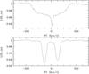 |
Fig. 9 LSD profiles from the TLS spectra of stars A (top) and B (bottom). |
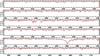 |
Fig. 10 Part of the TLS spectrum of V342 And (black) and the best-fit combination of synthetic spectra (red). |
The continuum flux ratio between the components is calculated in the following way. Let 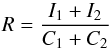 (2)be the observed spectrum normalized to the common continuum C1 + C2 of both stars, and f = C2/ (C1 + C2) be the flux ratio. Then we find
 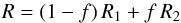 (3)where the Ri are the spectra normalized to the continua of the single components. Replacing the Ri by the synthetic spectra Si, we get
  (4)The flux ratio f can then be obtained from a least squares fit based on Eq. (4). Its wavelength dependence can be implemented by developing f into a polynomial in wavelength. We assumed a linear trend of f with wavelength.
Atmospheric parameters of binary star B derived from the composite spectrum and from the single spectra after disentangling.
After the determination of the best-fit synthetic spectra, we cleaned the observed, composite spectrum for the contribution of component 2 to get an approximation of component 1 and vice versa, using  (5)and analyzed the resulting single spectra separately. At this point, we were also able to iterate the abundances of single chemical elements. Table 6 lists the resulting atmospheric parameters. The given errors are 1σ errors derived from the full grid in all parameters per star and include all interdependencies between the parameters of one star. We had not enough computer power to include the errors arising from the interdependency between the two atmosphere models, however, so that the real errors may be slightly larger. The derived flux ratio is 0.45 ± 0.04. Table 7 lists the obtained abundances. The assumed solar values are given as log (Nel/Ntotal) and correspond to Barnes & Bash (2005). Figure 10 shows a part of the observed TLS spectrum together with the best-fit synthetic spectrum.
Derived abundances relative to the solar values.
A comparison of the results obtained from the composite and the single spectra (Table 6) shows that all values agree within their 1σ error bars. This is also the case when comparing the atmospheric parameters of the two stars, i.e., the two stars have the same properties within the measurement errors. The parameter errors obtained from the single spectra are slightly smaller, which is due to the fact that we additionally adjusted the abundances of the chemical elements. We could only determine the abundances with errors smaller than ±0.2 dex for Fe, Ni, Cr, and Mg. Both components of V342 And B show slight underabundances, with [M/H] of −0.1 dex. The abundances of all elements agree within their 1 σ error bars with this value.
We calculated the periods of rotation of both EB components, using vsini (Table 6), as well as radii and inclination from the Wilson-Devinney model (Table 5). We obtained values Trot1 = 2.45 ± 0.26d and Trot2 = 2.60 ± 0.32d, which denote a synchronous rotation.
There is an indication that Comp. 2 has slightly higher mass, but less flux in the optical range. This is hard to explain, however, and could be an over interpretation of the results. Our (conservative) conclusion is that all obtained parameters of the two stars agree within 2σ.
5. Conclusions
Multiple stars bring clues on star formation and evolution. Although in dense star clusters some binary stars may be formed dynamically through N-body interactions, the remaining binary and multiple systems are thought to form via fragmentation of the protostellar cloud. Recently it emerged that planets form in multiple systems through a process still less understood than multiple-star formation. Important practical use of detached binary stars is the top-precision distance indicator, based on binary parameter solutions. We look at multiple stellar systems from a different perspective, namely as test-beds of stellar evolution theory. Because of their identical age and composition, the components of multiple stars, particularly those near the main-sequence turnoff, yield sensitive tests of stellar evolution effects, such as age, metallicity, and convection efficiency. For that purpose one needs a precise solution for the binary parameters in multiple hierarchical star systems.
The main results of our investigation are the identification of the eclipsing component B of the visual binary and the determination of the absolute parameters of its both stars with accuracy for masses and radii less than 1%. We obtained a new light curve and first radial velocity curves with two spectroscopic instruments. Additionally, we determined the atmospheric parameters and the chemical abundances for the eclipsing binary.
The mass ratio between the two components in binary star B measured from the radial velocities is slightly above unity. This is at the limits of measuring accuracy, the difference in masses corresponds to the 1σ measurement error. From the mass ratio and the fact that we are dealing with a binary star, we expect to observe about the same log g (or only a slightly higher value for Comp. 2) and the same [Fe/H] and [M/H] for both components. This is exactly what we find from our spectrum analysis and we assume that the spectroscopic results should be reliable. On the other hand, we have no explanation for the significant difference between the Teff derived with the WD code from photometry and from spectrum analysis. If we place Comp. 1 on the evolutionary track that corresponds to its derived mass, the effective temperature calculated with WD for Comp. 2 is 170 K lower than the evolutionary model predicts. The distinctly higher Teff, as derived from the spectrum analysis, are not compatible with the mass-based evolutionary tracks of both components.
The LSD profile of star A suggests that it is a either a binary system or we observe a single star plus additional light from a field star.
IRAF is distributed by the National Optical Astronomy Observatory, which is operated by the Association of Universities for Research in Astronomy, Inc., under a cooperative agreement with the National Science Foundation.
Acknowledgments
We would like to thank Slavek M. Rucinski and DDO staff for generous hospitality. In particular, our team wants to express appreciation to the observers Heide DeBond and Jim Thomson. This work was supported by the Polish National Science Centre through grant UMO-2011/01/D/ST9/00427.
References
- Abt, H. A. 1981, ApJS, 45, 437 [NASA ADS] [CrossRef] [Google Scholar]
- Alzner, A. 1998, A&AS, 132, 237 [NASA ADS] [CrossRef] [EDP Sciences] [Google Scholar]
- Barnes, III, T. G., & Bash, F. N. 2005, in Cosmic Abundances as Records of Stellar Evolution and Nucleosynthesis in honor of David L. Lambert, ASP Conf. Ser., 336 [Google Scholar]
- Chambliss, C. R. 1992, PASP, 104, 663 [NASA ADS] [CrossRef] [Google Scholar]
- Dimitrov, W., Fagas, M., Kamiński, K., et al. 2014, A&A, 564, A26 [NASA ADS] [CrossRef] [EDP Sciences] [Google Scholar]
- Dommanget, J., & Nys, O. 1994, Communications de l’Observatoire Royal de Belgique, 115 [Google Scholar]
- Donati, J.-F., Semel, M., Carter, B. D., Rees, D. E., & Collier Cameron, A. 1997, MNRAS, 291, 658 [NASA ADS] [CrossRef] [MathSciNet] [Google Scholar]
- Duquennoy, A., & Mayor, M. 1991, A&A, 248, 485 [NASA ADS] [Google Scholar]
- Eggleton, P. P., & Kiseleva-Eggleton, L. 2001, ApJ, 562, 1012 [NASA ADS] [CrossRef] [Google Scholar]
- Hadrava, P. 1995, A&AS, 114, 393 [NASA ADS] [Google Scholar]
- Harrington, R. S. 1968, AJ, 73, 190 [NASA ADS] [CrossRef] [Google Scholar]
- Heintz, W. D. 1967, Journal des Observateurs, 50, 343 [NASA ADS] [Google Scholar]
- Kim, Y.-C., Demarque, P., Yi, S. K., & Alexander, D. R. 2002, ApJS, 143, 499 [NASA ADS] [CrossRef] [Google Scholar]
- Kozai, Y. 1962, AJ, 67, 591 [Google Scholar]
- Kupka, F., Piskunov, N., Ryabchikova, T. A., Stempels, H. C., & Weiss, W. W. 1999, A&AS, 138, 119 [NASA ADS] [CrossRef] [EDP Sciences] [MathSciNet] [PubMed] [Google Scholar]
- Lehmann, H., Tkachenko, A., Semaan, T., et al. 2011, A&A, 526, A124 [NASA ADS] [CrossRef] [EDP Sciences] [Google Scholar]
- Machida, M. N., Tomisaka, K., Matsumoto, T., & Inutsuka, S.-I. 2008, ApJ, 677, 327 [NASA ADS] [CrossRef] [Google Scholar]
- Mason, B. D., Wycoff, G. L., Hartkopf, W. I., Douglass, G. G., & Worley, C. E. 2001, AJ, 122, 3466 [Google Scholar]
- Mazeh, T., & Shaham, J. 1979, A&A, 77, 145 [Google Scholar]
- Pribulla, T., & Rucinski, S. M. 2006, AJ, 131, 2986 [NASA ADS] [CrossRef] [Google Scholar]
- Prša, A., & Zwitter, T. 2005, ApJ, 628, 426 [NASA ADS] [CrossRef] [Google Scholar]
- Pych, W. 2004, PASP, 116, 148 [NASA ADS] [CrossRef] [Google Scholar]
- Raghavan, D., McAlister, H. A., Henry, T. J., et al. 2010, ApJS, 190, 1 [NASA ADS] [CrossRef] [EDP Sciences] [Google Scholar]
- Rucinski, S. M. 1992, AJ, 104, 1968 [NASA ADS] [CrossRef] [Google Scholar]
- Rucinski, S. M. 2002, AJ, 124, 1746 [NASA ADS] [CrossRef] [Google Scholar]
- Schwarzenberg-Czerny, A. 1996, ApJ, 460, L107 [NASA ADS] [CrossRef] [Google Scholar]
- Sekalska, J., Dimitrov, W., Fagas, M., et al. 2010, IBVS, 5954, 1 [NASA ADS] [Google Scholar]
- Shulyak, D., Tsymbal, V., Ryabchikova, T., Stütz, C., & Weiss, W. W. 2004, A&A, 428, 993 [NASA ADS] [CrossRef] [EDP Sciences] [Google Scholar]
- Tkachenko, A., Lehmann, H., Smalley, B., Debosscher, J., & Aerts, C. 2012, MNRAS, 422, 2960 [NASA ADS] [CrossRef] [Google Scholar]
- Tokovinin, A., Thomas, S., Sterzik, M., & Udry, S. 2006, A&A, 450, 681 [NASA ADS] [CrossRef] [EDP Sciences] [Google Scholar]
- Tsymbal, V. 1996, in M.A.S.S., Model Atmospheres and Spectrum Synthesis, eds. S. J. Adelman, F. Kupka, & W. W. Weiss, ASP Conf. Ser., 108, 198 [Google Scholar]
- van Leeuwen, F. 2007, A&A, 474, 653 [NASA ADS] [CrossRef] [EDP Sciences] [Google Scholar]
- Wilson, R. E., & Devinney, E. J. 1971, ApJ, 166, 605 [NASA ADS] [CrossRef] [Google Scholar]
- Yi, S., Demarque, P., Kim, Y.-C., et al. 2001, ApJS, 136, 417 [NASA ADS] [CrossRef] [Google Scholar]
- Yi, S. K., Kim, Y.-C., & Demarque, P. 2003, ApJS, 144, 259 [NASA ADS] [CrossRef] [Google Scholar]
- Zahn, J.-P. 1975, A&A, 41, 329 [NASA ADS] [Google Scholar]
- Zahn, J.-P. 1977, A&A, 57, 383 [NASA ADS] [Google Scholar]
- Zasche, P., Wolf, M., Hartkopf, W. I., et al. 2009, AJ, 138, 664 [NASA ADS] [CrossRef] [Google Scholar]
- Zinnecker, H., & Mathieu, R. 2001, in The Formation of Binary Stars, IAU Symp., 200 [Google Scholar]
All Tables
Position angle and separation measurements from WDC and CCDM catalogs, Heintz (1967) and Alzner (1998).
Parameters of the eclipsing pair V342 Andromedae B obtained with Wilson-Devinney method.
Results of fitting only the spectroscopic data from DDO and PST1 and the formal errors.
Atmospheric parameters of binary star B derived from the composite spectrum and from the single spectra after disentangling.
All Figures
|
Fig. 1 Part of DDO spectrum, the plot shows two parallel spectra. Both visual components A and B are pointed on the slit. |
| In the text | |
|
Fig. 2 One of the well-exposed PST1 spectra with dissociated lines (HJD = 2 455 874.243). The hydrogen Hα and Hβ lines are plotted. |
| In the text | |
|
Fig. 3 Photometric data from our (top) and Hipparcos observations (bottom). The synthetic curves come from the fitted model. Hipparcos plot is shifted up by 0.1 mag. |
| In the text | |
|
Fig. 4 Radial velocity curve for V342 Andromedae B, the eclipsing pair. Open circles correspond to the DDO observations measured with the broadening function method. |
| In the text | |
|
Fig. 5 Four examples of cross-correlation function (PST1 spectra). The three peaks are marked, the central one is connected with the main visual component A. Outer peaks correspond to component B, the eclipsing pair. Horizontal axis shows the observed velocity and vertical axis the correlation coefficient. |
| In the text | |
|
Fig. 6 Radial velocity curves for all three components from PST1 triple-lined spectra. Dashed horizontal line presents the mean value of the third body (visual component A) radial velocity. |
| In the text | |
|
Fig. 7 Evolutionary tracks for both components of the eclipsing pair V342 And B. Solid lines present the tracks and dotted and dashed lines their error bars. The subframe shows the same curves zoomed out. Component 1 lays on its track and component 2 is shifted toward lower temperatures. |
| In the text | |
|
Fig. 8 Best fit (thick continuous line) of the LSD profile (thin) from one PST1 spectrum and the underlying double-Gaussian profiles for components A (dotted) and B (dashed). |
| In the text | |
|
Fig. 9 LSD profiles from the TLS spectra of stars A (top) and B (bottom). |
| In the text | |
|
Fig. 10 Part of the TLS spectrum of V342 And (black) and the best-fit combination of synthetic spectra (red). |
| In the text | |
Current usage metrics show cumulative count of Article Views (full-text article views including HTML views, PDF and ePub downloads, according to the available data) and Abstracts Views on Vision4Press platform.
Data correspond to usage on the plateform after 2015. The current usage metrics is available 48-96 hours after online publication and is updated daily on week days.
Initial download of the metrics may take a while.