| Issue |
A&A
Volume 575, March 2015
|
|
|---|---|---|
| Article Number | A61 | |
| Number of page(s) | 8 | |
| Section | Planets and planetary systems | |
| DOI | https://doi.org/10.1051/0004-6361/201423591 | |
| Published online | 24 February 2015 | |
WASP-20b and WASP-28b: a hot Saturn and a hot Jupiter in near-aligned orbits around solar-type stars ⋆,⋆⋆
1 Astrophysics Group, Keele University, Staffordshire ST5 5BG, UK
e-mail: This email address is being protected from spambots. You need JavaScript enabled to view it.
2 SUPA, School of Physics and Astronomy, University of St. Andrews, North Haugh, Fife KY16 9SS, UK
3 Observatoire de Genève, Université de Genève, 51 Chemin des Maillettes, 1290 Sauverny, Switzerland
4 Las Cumbres Observatory Global Telescope Network, 6740 Cortona Dr. Suite 102, Goleta, CA 93117, USA
5 Cavendish Laboratory, J J Thomson Avenue, Cambridge, CB3 0HE, UK
6 N. Copernicus Astronomical Centre, Polish Academy of Sciences, Bartycka 18, 00-716 Warsaw, Poland
7 Department of Physics, and Kavli Institute for Astrophysics and Space Research, MIT, Cambridge, MA 02139, USA
8 Department of Physics, University of Warwick, Coventry CV4 7AL, UK
9 Astrophysics Research Centre, School of Mathematics & Physics, Queen’s University, University Road, Belfast BT7 1NN, UK
10 Institut d’Astrophysique et de Géophysique, Université de Liège, Allée du 6 Août, 17, Bât. B5C, Liège 1, Belgium
Received: 6 February 2014
Accepted: 5 December 2014
Abstract
We report the discovery of the planets WASP-20b and WASP-28b along with measurements of their sky-projected orbital obliquities. WASP-20b is an inflated, Saturn-mass planet (0.31 MJup; 1.46 RJup) in a 4.9-day, near-aligned (λ = 12.7 ± 4.2°) orbit around CD-24 102 (V = 10.7; F9). Due to the low density of the planet and the apparent brightness of the host star, WASP-20 is a good target for atmospheric characterisation via transmission spectroscopy. WASP-28b is an inflated, Jupiter-mass planet (0.91 MJup; 1.21 RJup) in a 3.4-day, near-aligned (λ = 8 ± 18°) orbit around a V = 12, F8 star. As intermediate-mass planets in short orbits around aged, cool stars (7+ 2-1 Gyr and 6000 ± 100 K for WASP-20; 5+ 3-2 Gyr and 6100 ± 150 K for WASP-28), their orbital alignment is consistent with the hypothesis that close-in giant planets are scattered into eccentric orbits with random alignments, which are then circularised and aligned with their stars’ spins via tidal dissipation.
Key words: planetary systems / stars: individual: WASP-20b / stars: individual: WASP-28b
Based on observations made with: the WASP-South (South Africa) and SuperWASP-North (La Palma) photometric survey instruments; the C2 and EulerCam cameras and the CORALIE spectrograph, all mounted on the 1.2-m Euler-Swiss telescope (La Silla); the HARPS spectrograph on the ESO 3.6-m telescope (La Silla) under programs 072.C-0488, 082.C-0608, 084.C-0185, and 085.C-0393; and LCOGT’s Faulkes Telescope North (Maui) and Faulkes Telescope South (Siding Spring).
Full Tables 2 and 3 are only available at the CDS via anonymous ftp to cdsarc.u-strasbg.fr (130.79.128.5) or via http://cdsarc.u-strasbg.fr/viz-bin/qcat?J/A+A/575/A61
© ESO, 2015
1. Introduction
Planets that transit relatively bright host stars (V< 13) are proving a rich source of information for the nascent field of exoplanetology. To date, the main discoverers of these systems are the ground-based transit surveys HATNet and SuperWASP and the space mission Kepler (Bakos et al., 2004; Pollacco et al., 2006; Borucki et al., 2010).
Summary of observations.
One parameter that, uniquely, we can determine for transiting planets is obliquity (Ψ), the angle between a star’s rotation axis and a planet’s orbital axis. We do this by taking spectra of a star during transit: as the planet obscures a portion of the rotating star it causes a distortion of the observed stellar line profile, which manifests as an anomalous radial-velocity (RV) signature known as the Rossiter-McLaughlin (RM) effect (Rossiter, 1924; McLaughlin, 1924). The shape of the RM effect is sensitive to the path a planet takes across the disc of a star relative to the stellar spin axis. If we have a constraint on the inclination of the stellar spin axis relative to the sky plane (I∗), then we can determine the true obliquity (Ψ), otherwise we can only determine the sky-projected obliquity (λ). The two are related by:  where iP is the inclination of the orbital axis to the sky plane.
The obliquity of a short-period, giant planet may be indicative of the manner in which it arrived in its current orbit from farther out, where it presumably formed. As the angular momenta of a star and its planet-forming disc both derive from that of their parent molecular cloud, stellar spin and planetary orbital axes are expected to be, at least initially, aligned. Migration via tidal interaction with the gas disc is expected to preserve initial spin-orbit alignment (Lin et al., 1996; Marzari & Nelson, 2009), but almost half (33 of 74) of the orbits so far measured are misaligned and approximately 10 of those are retrograde1.
These results are consistent with the hypothesis that some or all close-in giant planets arrive in their orbits by planet-planet and/or star-planet scattering, which can drive planets into eccentric, misaligned orbits, and tidal friction, which circularises, shortens and aligns orbits (see the following empirical-based papers: Triaud et al. 2010; Winn et al. 2010; Naoz et al. 2011; Albrecht et al. 2012; also see the following model-based papers: Fabrycky & Tremaine 2007; Nagasawa et al. 2008; Matsumura et al. 2010; Naoz et al. 2011).
Systems with short tidal timescales (those with short scaled orbital major semi-axes, a/R∗, and high planet-to-star mass ratios) tend to be aligned (Albrecht et al. 2012, and references therein). A broad range of obliquities is observed for stars with Teff> 6250 K, for which tidal realignment processes may be inefficient due to the absence of a substantial convective envelope (Winn et al., 2010; Schlaufman, 2010). Limiting focus to stars more massive than 1.2 M⊙, for which age determinations are more reliable, Triaud (2011) noted that systems older than 2.5 Gyr tend to be aligned; this could be indicative of the time required for orbital alignment or of the timescale over which hotter stars develop a substantial convective envelope as they evolve.
A major hurdle to overcome for any hypothesis involving realignment is tidal dissipation seems to cause both orbital decay and realignment on similar timescales (Barker & Ogilvie, 2009). Alternative hypotheses suggest that misalignments arise via reorientations of either the disc or the stellar spin and that migration then proceeds via planet-disc interactions (e.g. Bate et al. 2010; Lai et al. 2011; Rogers et al. 2012). However, observations of discs well-aligned with their stellar equators suggest that tilting of the star or the disc rarely occurs (Watson et al., 2011; Greaves et al., 2014).
Here we present the discovery and obliquity determinations of the planets transiting the stars WASP-20 (CD-24 102) and WASP-28 (2MASS J23342787−0134482), and we interpret the results under the hypothesis of migration via scattering and tidal dissipation.
2. Observations
We provide a summary of observations in Table 1. The WASP (Wide Angle Search for Planets) photometric survey (Pollacco et al., 2006) monitors bright stars (V = 9.5–13.5) using two eight-camera arrays, each with a field of view of 450 deg2. Each array observes up to eight pointings per night with a cadence of 5–10 min, and each pointing is followed for around five months per season. The WASP-South station (Hellier et al., 2011) is hosted by the South African Astronomical Observatory and the SuperWASP-North station (Faedi et al., 2011) is hosted by the Isaac Newton Group at the Observatorio del Roque de Los Muchachos on La Palma. The WASP data were processed and searched for transit signals as described in Collier Cameron et al. (2006) and the candidate selection process was performed as described in Collier Cameron et al. (2007). We observed periodic dimmings in the WASP lightcurves of WASP-20 and WASP-28 with periods of 4.8996 d and 3.4088 d, respectively (see the top panels of Figs. 1 and 2). We searched the WASP lightcurves for modulation as could be caused by magnetic activity and stellar rotation (Maxted et al., 2011). We did not detect any significant, repeated signals and we find that any modulation must be below the 2-mmag level.
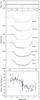 |
Fig. 1 WASP-20b discovery data. Top panel: WASP lightcurve folded on the transit ephemeris. Middle panel: transit lightcurves from facilities as labelled, offset for clarity and binned with a bin width of two minutes. The best-fitting transit model is superimposed. Bottom panel: the radial velocities (CORALIE in blue, HARPS in green and HARPS covering the transit in brown) with the best-fitting circular Keplerian orbit model and the RM effect model. |
We obtained 56 spectra of WASP-20 and 26 spectra of WASP-28 with the CORALIE spectrograph mounted on the Euler-Swiss 1.2-m telescope (Baranne et al., 1996; Queloz et al., 2000). We obtained a further 63 spectra of WASP-20 with the HARPS spectrograph mounted on the 3.6-m ESO telescope (Mayor et al., 2003), including a sequence of 43 spectra taken through the transit of the night of 2009 October 22. We obtained a further 33 spectra of WASP-28 with HARPS, including 30 spectra taken through the transit of the night of 2010 August 17. Radial-velocity measurements were computed by weighted cross-correlation (Baranne et al., 1996; Pepe et al., 2005) with a numerical G2-spectral template (Table 2). We detected RV variations with periods similar to those found from the WASP photometry and with semi-amplitudes consistent with planetary-mass companions. We plot the RVs, phased on the transit ephemerides, in the third panel of Figs. 1 and 2 and we highlight the RM effects in Fig. 3.
For each star, we tested the hypothesis that the RV variations are due to spectral-line distortions caused by a blended eclipsing binary or starspots by performing a line-bisector analysis of the cross-correlation functions (Queloz et al., 2001). The lack of any significant correlation between bisector span and RV supports our conclusion that the periodic dimming and RV variation of each system are caused by a transiting planet (Fig. 4). This is further supported by our observation of the RM effect of each system: the vsinI∗ values from our fits to the RM effects are consistent with the values we obtain from spectral line broadening (see Sects. 3 and 4).
We performed follow-up transit observations to refine the systems’ parameters using the Euler-Swiss 1.2-m telescope (Lendl et al., 2012), and LCOGT’s 2.0-m Faulkes Telescopes North and South (Brown et al., 2013) (see the middle panels of Figs. 1 and 2). Some transit lightcurves were affected by technical problems or poor weather, as indicated in Table 1.
Radial-velocity measurements.
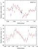 |
Fig. 3 Rossiter-McLaughlin effects, or spectroscopic transits, of WASP-20b and WASP-28b. The CORALIE RVs are shown in blue and the HARPS RVs are shown in brown. The Keplerian orbits have been subtracted. For each planet, the observed apparent redshift, followed by an apparent blueshift of similar amplitude, indicate the orbit to be prograde and, probably, aligned with the stellar rotation. The alignment of the orbit of WASP-28b is less certain due to its low impact parameter. The lower precision of the earlier WASP-28 RVs resulted because the sequence started at an airmass of 1.7. |
Follow-up photometry.
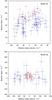 |
Fig. 4 The lack of any significant correlation between bisector span and radial velocity excludes transit mimics and supports our conclusion that each system contains a transiting planet. |
3. Stellar parameters from spectra
The 9 individual HARPS spectra from 2008 of WASP-20 were co-added and a total of 18 individual CORALIE spectra of WASP-28 were co-added to produce one spectrum per star, with typical signal-to-noise ratio of 150:1 (WASP-20) and 70:1 (WASP-28). The standard pipeline reduction products were used in the analysis.
The analysis was performed using the methods given in Gillon et al. (2009). The Hα line was used to determine the effective temperature (Teff), while the Na i D and Mg i b lines were used as surface gravity (log g∗) diagnostics. The parameters obtained from the analysis are listed in Table 4. The elemental abundances were determined from equivalent width measurements of several clean and unblended lines. A value for microturbulence (ξt) was determined from Fe i using the method of Magain (1984). The quoted error estimates include that given by the uncertainties in Teff, log g∗ and ξt, as well as the scatter due to measurement and atomic data uncertainties.
We assumed values for macroturbulence (vmac) of 4.5 ± 0.3 km s-1 and 4.7 ± 0.3 km s-1 for WASP-20 and WASP-28, respectively. These were based on the tabulation by Gray (2008) and the instrumental FWHMs of 0.065 Å (HARPS) and 0.11 ± 0.01 Å (CORALIE), as determined from the telluric lines around 6300 Å. We determined the projected stellar rotation velocity (vsinI∗) by fitting the profiles of several unblended Fe i lines. We determined the vsinI∗ of WASP-20 from the 62 HARPS spectra obtained up to 2010 and the vsinI∗ of WASP-28 from all 33 available HARPS spectra.
Stellar parameters from the spectra.
4. System parameters from the RV and transit data
We determined the parameters of each system from a simultaneous fit to the lightcurve and RV data. The fit was performed using the current version of the Markov-chain Monte Carlo (MCMC) code described by Collier Cameron et al. (2007) and Pollacco et al. (2008).
The transit lightcurves are modelled using the formulation of Mandel & Agol (2002) with the assumption that the planet is much smaller than the star. Limb-darkening was accounted for using a four-coefficient, nonlinear limb-darkening model, using coefficients appropriate to the passbands from the tabulations of Claret (2000, 2004). The coefficients are interpolated once using the values of log g∗ and [Fe/H] in Table 4, but are interpolated at each MCMC step using the latest value of Teff. The coefficient values corresponding to the best-fitting value of Teff are given in Table 5. The transit lightcurve is parameterised by the epoch of mid-transit T0, the orbital period P, the planet-to-star area ratio (RP/R∗)2, the approximate duration of the transit from initial to final contact T14, and the impact parameter b = acosiP/R∗ (the distance, in fractional stellar radii, of the transit chord from the star’s centre in the case of a circular orbit), where a is the semimajor axis and iP is the inclination of the orbital plane with respect to the sky plane.
Limb-darkening coefficients.
System parameters from the MCMC analyses.
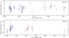 |
Fig. 5 Residuals about the best-fitting Keplerian orbits as a function of time (CORALIE in blue, HARPS in green, and HARPS transits in brown). There is no evidence of additional bodies. |
The eccentric Keplerian RV orbit is parameterised by the stellar reflex velocity semi-amplitude K1, the systemic velocity γ, an instrumental offset between the HARPS and CORALIE spectrographs ΔγHARPS, and  and
and  where e is orbital eccentricity and ω is the argument of periastron. We use and as they impose a uniform prior on e, whereas the jump parameters we used previously, ecosω and esinω, impose a linear prior that biases e toward higher values (Anderson et al., 2011b). The RM effect was modelled using the formulation of Ohta et al. (2005) and, for similar reasons, is parameterised by
  and
and  .
.
The linear scale of the system depends on the orbital separation a which, through Kepler’s third law, depends on the stellar mass M∗. At each step in the Markov chain, the latest values of ρ∗, Teff and [Fe/H] are input in to the empirical mass calibration of Enoch et al. (2010) (as based upon Torres et al. 2010, and as updated by Southworth 2011) to obtain M∗. The shapes of the transit lightcurves and the RV curve constrain stellar density ρ∗ (Seager & Mallén-Ornelas, 2003), which combines with M∗ to give the stellar radius R∗. The stellar effective temperature Teff and metallicity [Fe/H] are proposal parameters constrained by Gaussian priors with mean values and variances derived directly from the stellar spectra (see Sect. 3).
As the planet-to-star area ratio is determined from the measured transit depth, the planet radius RP follows from R∗. The planet mass MP is calculated from the measured value of K1 and the value of M∗; the planetary density ρP and surface gravity log gP then follow. We calculate the planetary equilibrium temperature Teql, assuming zero albedo and efficient redistribution of heat from the planet’s presumed permanent day side to its night side. We also calculate the durations of transit ingress (T12) and egress (T34).
At each step in the MCMC procedure, model transit lightcurves and RV curves are computed from the proposal parameter values, which are perturbed from the previous values by a small, random amount. The χ2 statistic is used to judge the goodness of fit of these models to the data and the decision as to whether to accept a step is made via the Metropolis-Hastings rule (Collier Cameron et al., 2007): a step is accepted if χ2 is lower than for the previous step and a step with higher χ2 is accepted with a probability proportional to exp( − Δχ2/ 2). This gives the procedure some robustness against local minima and results in a thorough exploration of the parameter space around the best-fitting solution. To give proper weighting to each photometric data set, the uncertainties were scaled at the start of the MCMC so as to obtain a photometric reduced-χ2 of unity. To obtain a spectroscopic reduced-χ2 of unity we added “jitter” terms in quadrature to the formal RV errors of WASP-20: 12 m s-1 for the CORALIE RVs and 7 m s-1 for the HARPS RVs; no jitter was required for WASP-28. To account for e.g. a specific activity level, we partitioned the HARPS RVs of WASP-20 into two sets: those taken on the night of the spectroscopic transit observation of 2009 Oct. 22 and the remainder.
For both WASP-20b and WASP-28b we find, using the F-test approach of Lucy & Sweeney (1971), that the improvement in the fit to the RV data resulting from the use of an eccentric orbit model is small and is consistent with the underlying orbit being circular. We thus adopt circular orbits, which Anderson et al. (2012) suggest is the prudent choice for short-period, ~Jupiter-mass planets in the absence of evidence to the contrary. We find 2σ upper limits on e of 0.11 and 0.14 for WASP-20b and WASP-28b, respectively.
Due to the low impact parameter of WASP-28b determinations of vsinI∗ and λ are degenerate (Triaud et al., 2011; Albrecht et al., 2011; Anderson et al., 2011a). To ensure vsinI∗ is consistent with our spectroscopic measurement, we imposed a Gaussian prior on it by means of a Bayesian penalty on χ2, with mean and variance as determined from the HARPS spectra (see Sect. 3). From an MCMC run with no prior we obtained λ = −8 ± 54° and vsinI∗ km s-1, with vsinI∗ reaching values as high as 30 km s-1, which is clearly inconsitent with the spectral measurement of vsinI∗= 3.1 ± 0.6 km s-1. The degeneracy between vsinI∗ and λ could be broken by line-profile tomography (Albrecht et al., 2007; Collier Cameron et al., 2010).
The median values and the 1σ limits of our MCMC parameters’ posterior distributions are given in Table 6 along with those of the derived parameters. The best fits to the RVs and the photometry are plotted in Figs. 1 and 2, with the RM effects highlighted in Fig. 3. There is no evidence of additional bodies in the RV residuals (Fig. 5).
We interpolated the mass tracks of Bertelli et al. (2008) and the isochrones of Bressan et al. (2012) using ρ∗, Teff and [Fe/H] from the MCMC analysis (Fig. 6). This suggests ages of  Gyr for WASP-20 and
  Gyr for WASP-28 and masses of
  M⊙ for WASP-20 and 0.91 ± 0.06 M⊙ for WASP-28. These are slightly lower than the masses derived from our MCMC analyses (1.20 ± 0.04 M⊙ for WASP-20 and 1.02 ± 0.05 M⊙ for WASP-28), though they are consistent at the 2.3σ (WASP-20) and 1.4σ (WASP-28) levels. This discrepancy between these mass estimates suggests that there may be additional factors not accounted for in the stellar models. It is not possible to quantify the additional uncertainty on the mass and age derived from the models without knowing the reason(s) for this discrepancy. It is also possible that these stars differ in some way from those used to establish the empirical mass calibration used in our MCMC analysis. This is certainly an interesting problem that warrants further investigation, but it is beyond the scope of this paper.
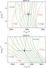 |
Fig. 6 Modified H–R diagrams. The isochrones, from Bressan et al. (2012), are in steps of integer Gyr with Z = 0.0152 for WASP-20 and Z = 0.0078 for WASP-28. The mass tracks, from Bertelli et al. (2008), are in steps of 0.1 M⊙ with Z = 0.019 for WASP-20 and Z = 0.0097 for WASP-28. |
5. Discussion
We present the discovery of WASP-20b, a Saturn-mass planet in a 4.9-day orbit around CD-24 102 (V = 10.7), and WASP-28b, a Jupiter-mass planet in a 3.4-day orbit around a V = 12 star. Based on their masses, orbital distances, irradiation levels and metallicities, the radii of the planets (1.46 RJup for WASP-20b and 1.21 RJup for WASP-28b) are consistent with the predictions of the empirical relations of Enoch et al. (2012): 1.33 RJup for WASP-20b and 1.26 RJup for WASP-28b. Due to the low density of the planet and the apparent brightness of its host star, WASP-20 is a good target for atmospheric characterisation via transmission spectroscopy (e.g. Kreidberg et al. 2014).
We find both WASP-20b and WASP-28b to be in prograde orbits. The orbit of WASP-20b may be slightly misaligned with its star’s spin: λ = 12.7 ± 4.2°. Although our measurement for WASP-28b (λ = 8 ± 18°) is consistent with an aligned orbit, its low impact parameter results in a relatively large uncertainty. Using the period-colour relation for the Hyades of Delorme et al. (2011) and scaling to the inferred ages of the host stars using P ∝ t0.5, we predict rotation velocities consistent with the spectroscopic vsinI∗ values: v ~ 2.9 km s-1 for WASP-20 and v ~ 2.1 km s-1 for WASP-28. This suggests that I∗ ≈ 90° and therefore that Ψ ≈ λ.
Both host stars are near the posited boundary between efficient and inefficient aligners of Teff≈ 6250 K (Winn et al., 2010; Schlaufman, 2010). Both systems, with their low obliquity determinations, are consistent with the observation that systems with cool host stars and short expected tidal timescales are aligned (Albrecht et al. 2012, and references therein). With MP/M∗ = 0.00025 and a/R∗ = 9.3, WASP-20b experiences relatively weak tidal forces. Its relative tidal dissipation timescale of τCE = 2.6 × 10¹³ yr is the longest for the cool-host group barring HD 17156 b (see Sect. 5.3 of Albrecht et al. 2012)2. With MP/M∗ = 0.00084 and a/R∗ = 9.5, τCE = 2.5 × 10¹² yr for WASP-28b, placing it within the main grouping of aligned, cool-host systems. Assuming the planets did not arrive in their current orbits recently, the advanced age of both systems, Gyr for WASP-20 and Gyr for WASP-28, mean tidal dissipation would have occurred over a long timescale.
The planets may have arrived in their current orbits via planet-disc migration (Lin et al., 1996; Marzari & Nelson, 2009) or via the scattering and circularisation route (Fabrycky & Tremaine, 2007; Nagasawa et al., 2008; Matsumura et al., 2010; Naoz et al., 2011). Assuming the latter, the planets may have scattered into near-aligned orbits or they may have aligned with the spins of their host stars via tidal interaction, though how this could have occurred without the planets falling into their stars is currently a mystery (Barker & Ogilvie, 2009). It will be interesting to discover if the small, significant misalignment of WASP-20 is confirmed by further observations and, perhaps, by a re-analysis of the existing data using the line-profile tomography technique (Albrecht et al., 2007; Collier Cameron et al., 2010). In that case the system may prove particularly useful in studies of the migration of hot Jupiters and the tidal damping of spin-orbit misalignments.
René Heller maintains a list of measurements and references at http://www.physics.mcmaster.ca/~rheller/content/main_HRM.html
Note that these timescales are relative and that Albrecht et al. (2012) plot the timescales divided by 5 × 10⁹.
Acknowledgments
WASP-South is hosted by the South African Astronomical Observatory and SuperWASP-North is hosted by the Isaac Newton Group on La Palma. We are grateful for their ongoing support and assistance. Funding for WASP comes from consortium universities and from the UK’s Science and Technology Facilities Council. M. Gillon is a FNRS Research Associate. A. H. M. J. Triaud is a Swiss National Science Foundation fellow under grant number PBGEP2-145594.
References
- Albrecht, S., Reffert, S., Snellen, I., Quirrenbach, A., & Mitchell, D. S. 2007, A&A, 474, 565 [NASA ADS] [CrossRef] [EDP Sciences] [Google Scholar]
- Albrecht, S., Winn, J. N., Johnson, J. A., et al. 2011, ApJ, 738, 50 [NASA ADS] [CrossRef] [Google Scholar]
- Albrecht, S., Winn, J. N., Johnson, J. A., et al. 2012, ApJ, 757, 18 [NASA ADS] [CrossRef] [Google Scholar]
- Anderson, D. R., Collier Cameron, A., Gillon, M., et al. 2011a, A&A, 534, A16 [NASA ADS] [CrossRef] [EDP Sciences] [Google Scholar]
- Anderson, D. R., Collier Cameron, A., Hellier, C., et al. 2011b, ApJ, 726, L19 [NASA ADS] [CrossRef] [Google Scholar]
- Anderson, D. R., Collier Cameron, A., Gillon, M., et al. 2012, MNRAS, 422, 1988 [NASA ADS] [CrossRef] [Google Scholar]
- Bakos, G., Noyes, R. W., Kovács, G., et al. 2004, PASP, 116, 266 [NASA ADS] [CrossRef] [Google Scholar]
- Baranne, A., Queloz, D., Mayor, M., et al. 1996, A&AS, 119, 373 [NASA ADS] [CrossRef] [EDP Sciences] [Google Scholar]
- Barker, A. J., & Ogilvie, G. I. 2009, MNRAS, 395, 2268 [NASA ADS] [CrossRef] [Google Scholar]
- Bate, M. R., Lodato, G., & Pringle, J. E. 2010, MNRAS, 401, 1505 [NASA ADS] [CrossRef] [Google Scholar]
- Bertelli, G., Girardi, L., Marigo, P., & Nasi, E. 2008, A&A, 484, 815 [NASA ADS] [CrossRef] [EDP Sciences] [Google Scholar]
- Borucki, W. J., Koch, D., Basri, G., et al. 2010, Science, 327, 977 [NASA ADS] [CrossRef] [PubMed] [Google Scholar]
- Bressan, A., Marigo, P., Girardi, L., et al. 2012, MNRAS, 427, 127 [NASA ADS] [CrossRef] [Google Scholar]
- Brown, T. M., Baliber, N., Bianco, F. B., et al. 2013, PASP, 125, 1031 [NASA ADS] [CrossRef] [Google Scholar]
- Claret, A. 2000, A&A, 363, 1081 [NASA ADS] [Google Scholar]
- Claret, A. 2004, A&A, 428, 1001 [NASA ADS] [CrossRef] [EDP Sciences] [Google Scholar]
- Collier Cameron, A., Pollacco, D., Street, R. A., et al. 2006, MNRAS, 373, 799 [NASA ADS] [CrossRef] [Google Scholar]
- Collier Cameron, A., Wilson, D. M., West, R. G., et al. 2007, MNRAS, 380, 1230 [NASA ADS] [CrossRef] [Google Scholar]
- Collier Cameron, A., Bruce, V. A., Miller, G. R. M., Triaud, A. H. M. J., & Queloz, D. 2010, MNRAS, 403, 151 [NASA ADS] [CrossRef] [Google Scholar]
- Delorme, P., Collier Cameron, A., Hebb, L., et al. 2011, MNRAS, 413, 2218 [NASA ADS] [CrossRef] [Google Scholar]
- Enoch, B., Collier Cameron, A., Parley, N. R., & Hebb, L. 2010, A&A, 516, A33 [NASA ADS] [CrossRef] [EDP Sciences] [Google Scholar]
- Enoch, B., Collier Cameron, A., & Horne, K. 2012, A&A, 540, A99 [NASA ADS] [CrossRef] [EDP Sciences] [Google Scholar]
- Fabrycky, D., & Tremaine, S. 2007, ApJ, 669, 1298 [NASA ADS] [CrossRef] [Google Scholar]
- Faedi, F., Barros, S. C. C., Pollacco, D., et al. 2011, Detection and Dynamics of Transiting Exoplanets, St. Michel l’Observatoire, France, eds. F. Bouchy, R. Díaz, & C. Moutou, EPJ Web Conf., 11, 1003 [Google Scholar]
- Gray, D. F. 2008, The Observation and Analysis of Stellar Photospheres (Cambridge University Press) [Google Scholar]
- Greaves, J. S., Kennedy, G. M., Thureau, N., et al. 2014, MNRAS, 438, L31 [NASA ADS] [CrossRef] [Google Scholar]
- Hellier, C., Anderson, D. R., Collier Cameron, A., et al. 2011, Detection and Dynamics of Transiting Exoplanets, St. Michel l’Observatoire, France, eds. F. Bouchy, R. Díaz, & C. Moutou, EPJ Web Conf., 11, 1004 [Google Scholar]
- Kreidberg, L., Bean, J. L., Désert, J.-M., et al. 2014, ApJ, 793, L27 [NASA ADS] [CrossRef] [Google Scholar]
- Lai, D., Foucart, F., & Lin, D. N. C. 2011, MNRAS, 412, 2790 [NASA ADS] [CrossRef] [Google Scholar]
- Lendl, M., Anderson, D. R., Collier-Cameron, A., et al. 2012, A&A, 544, A72 [NASA ADS] [CrossRef] [EDP Sciences] [Google Scholar]
- Lin, D. N. C., Bodenheimer, P., & Richardson, D. C. 1996, Nature, 380, 606 [NASA ADS] [CrossRef] [Google Scholar]
- Lucy, L. B., & Sweeney, M. A. 1971, AJ, 76, 544 [NASA ADS] [CrossRef] [Google Scholar]
- Magain, P. 1984, A&A, 134, 189 [NASA ADS] [Google Scholar]
- Mandel, K., & Agol, E. 2002, ApJ, 580, L171 [NASA ADS] [CrossRef] [Google Scholar]
- Marzari, F., & Nelson, A. F. 2009, ApJ, 705, 1575 [NASA ADS] [CrossRef] [Google Scholar]
- Matsumura, S., Peale, S. J., & Rasio, F. A. 2010, ApJ, 725, 1995 [NASA ADS] [CrossRef] [Google Scholar]
- Maxted, P. F. L., Anderson, D. R., Collier Cameron, A., et al. 2011, PASP, 123, 547 [NASA ADS] [CrossRef] [Google Scholar]
- Mayor, M., Pepe, F., Queloz, D., et al. 2003, The Messenger, 114, 20 [NASA ADS] [Google Scholar]
- McLaughlin, D. B. 1924, ApJ, 60, 22 [NASA ADS] [CrossRef] [Google Scholar]
- Nagasawa, M., Ida, S., & Bessho, T. 2008, ApJ, 678, 498 [NASA ADS] [CrossRef] [Google Scholar]
- Naoz, S., Farr, W. M., Lithwick, Y., Rasio, F. A., & Teyssandier, J. 2011, Nature, 473, 187 [NASA ADS] [CrossRef] [Google Scholar]
- Ohta, Y., Taruya, A., & Suto, Y. 2005, ApJ, 622, 1118 [NASA ADS] [CrossRef] [Google Scholar]
- Pepe, F., Mayor, M., Queloz, D., et al. 2005, The Messenger, 120, 22 [NASA ADS] [Google Scholar]
- Pollacco, D. L., Skillen, I., Cameron, A. C., et al. 2006, PASP, 118, 1407 [NASA ADS] [CrossRef] [Google Scholar]
- Pollacco, D., Skillen, I., Collier Cameron, A., et al. 2008, MNRAS, 385, 1576 [NASA ADS] [CrossRef] [Google Scholar]
- Queloz, D., Mayor, M., Weber, L., et al. 2000, A&A, 354, 99 [NASA ADS] [Google Scholar]
- Queloz, D., Henry, G. W., Sivan, J. P., et al. 2001, A&A, 379, 279 [NASA ADS] [CrossRef] [EDP Sciences] [Google Scholar]
- Rogers, T. M., Lin, D. N. C., & Lau, H. H. B. 2012, ApJ, 758, L6 [NASA ADS] [CrossRef] [Google Scholar]
- Rossiter, R. A. 1924, ApJ, 60, 15 [NASA ADS] [CrossRef] [Google Scholar]
- Schlaufman, K. C. 2010, ApJ, 719, 602 [NASA ADS] [CrossRef] [Google Scholar]
- Seager, S., & Mallén-Ornelas, G. 2003, ApJ, 585, 1038 [NASA ADS] [CrossRef] [Google Scholar]
- Southworth, J. 2011, MNRAS, 417, 2166 [NASA ADS] [CrossRef] [Google Scholar]
- Torres, G., Andersen, J., & Giménez, A. 2010, A&ARv, 18, 67 [Google Scholar]
- Triaud, A. H. M. J. 2011, A&A, 534, L6 [NASA ADS] [CrossRef] [EDP Sciences] [Google Scholar]
- Triaud, A. H. M. J., Collier Cameron, A., Queloz, D., et al. 2010, A&A, 524, A25 [NASA ADS] [CrossRef] [EDP Sciences] [Google Scholar]
- Triaud, A. H. M. J., Queloz, D., Hellier, C., et al. 2011, A&A, 531, A24 [NASA ADS] [CrossRef] [EDP Sciences] [Google Scholar]
- Watson, C. A., Littlefair, S. P., Diamond, C., et al. 2011, MNRAS, 413, L71 [NASA ADS] [CrossRef] [Google Scholar]
- Winn, J. N., Fabrycky, D., Albrecht, S., & Johnson, J. A. 2010, ApJ, 718, L145 [NASA ADS] [CrossRef] [Google Scholar]
- Zacharias, N., Monet, D. G., Levine, S. E., et al. 2004, BAAS, 36, 1418 [Google Scholar]
All Tables
All Figures
|
Fig. 1 WASP-20b discovery data. Top panel: WASP lightcurve folded on the transit ephemeris. Middle panel: transit lightcurves from facilities as labelled, offset for clarity and binned with a bin width of two minutes. The best-fitting transit model is superimposed. Bottom panel: the radial velocities (CORALIE in blue, HARPS in green and HARPS covering the transit in brown) with the best-fitting circular Keplerian orbit model and the RM effect model. |
| In the text | |
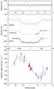 |
Fig. 2 WASP-28b discovery data. Caption as for Fig. 1. |
| In the text | |
|
Fig. 3 Rossiter-McLaughlin effects, or spectroscopic transits, of WASP-20b and WASP-28b. The CORALIE RVs are shown in blue and the HARPS RVs are shown in brown. The Keplerian orbits have been subtracted. For each planet, the observed apparent redshift, followed by an apparent blueshift of similar amplitude, indicate the orbit to be prograde and, probably, aligned with the stellar rotation. The alignment of the orbit of WASP-28b is less certain due to its low impact parameter. The lower precision of the earlier WASP-28 RVs resulted because the sequence started at an airmass of 1.7. |
| In the text | |
|
Fig. 4 The lack of any significant correlation between bisector span and radial velocity excludes transit mimics and supports our conclusion that each system contains a transiting planet. |
| In the text | |
|
Fig. 5 Residuals about the best-fitting Keplerian orbits as a function of time (CORALIE in blue, HARPS in green, and HARPS transits in brown). There is no evidence of additional bodies. |
| In the text | |
|
Fig. 6 Modified H–R diagrams. The isochrones, from Bressan et al. (2012), are in steps of integer Gyr with Z = 0.0152 for WASP-20 and Z = 0.0078 for WASP-28. The mass tracks, from Bertelli et al. (2008), are in steps of 0.1 M⊙ with Z = 0.019 for WASP-20 and Z = 0.0097 for WASP-28. |
| In the text | |
Current usage metrics show cumulative count of Article Views (full-text article views including HTML views, PDF and ePub downloads, according to the available data) and Abstracts Views on Vision4Press platform.
Data correspond to usage on the plateform after 2015. The current usage metrics is available 48-96 hours after online publication and is updated daily on week days.
Initial download of the metrics may take a while.