| Issue |
A&A
Volume 575, March 2015
|
|
|---|---|---|
| Article Number | A64 | |
| Number of page(s) | 13 | |
| Section | Stellar structure and evolution | |
| DOI | https://doi.org/10.1051/0004-6361/201323136 | |
| Published online | 24 February 2015 | |
Efficiency of ETV diagrams as diagnostic tools for long-term period variations
II. Non-conservative mass transfer, and gravitational radiation
1 Department of Astrophysics, Astronomy and MechanicsFaculty of Physics, National and Kapodistrian University of Athens, Panepistimiopolis Zografou, 15 784 Athens, Greece
e-mail: nanouris@phys.uoa.gr; eantonop@phys.uoa.gr; elivan@phys.uoa.gr
2 Department of Environment Technologists, School of Technological Applications, Technological and Educational Institute of Ionian Islands, Panagoula, 29 100 Zakynthos, Greece
e-mail: taskal@teiion.gr
3 Institute for Astronomy, Astrophysics, Space Applications and Remote Sensing, National Observatory of Athens, I. Metaxa & Vas. Pavlou St., Palaia Penteli, 15 236 Athens, Greece
Received: 27 November 2013
Accepted: 1 November 2014
Context. The credibility of an eclipse timing variation (ETV) diagram analysis is investigated for various manifestations of the mass transfer and gravitational radiation processes in binary systems. The monotonicity of the period variations and the morphology of the respective ETV diagrams are thoroughly explored in both the direct impact and the accretion disk mode of mass transfer, accompanied by different types of mass and angular momentum losses (through a hot-spot emission from the gainer and via the L2/L3 points).
Aims. Our primary objective concerns the traceability of each physical mechanism by means of an ETV diagram analysis. Also, possible critical mass ratio values are sought for those transfer modes that involve orbital angular momentum losses strong enough to dictate the secular period changes even when highly competitive mechanisms with the opposite direction act simultaneously.
Methods. The  relation that governs the orbital evolution of a binary system is set to provide the exact solution for the period and the function expected to represent the subsequent eclipse timing variations. The angular momentum transport is parameterized through appropriate empirical relations, which are inferred from semi-analytical ballistic models. Then, we numerically determine the minimum temporal range over which a particular mechanism is rendered measurable, as well as the critical mass ratio values that signify monotonicity inversion in the period modulations.
Results. Mass transfer rates comparable to or greater than 10-8 M⊙ yr-1 are measurable for typical noise levels of the ETV diagrams, regardless of whether the process is conservative. However, the presence of a transient disk around the more massive component defines a critical mass ratio (qcr ≈ 0.83) above which the period turns out to decrease when still in the conservative regime, rendering the measurability of the anticipated variations a much more complicated task. The effects of gravitational radiation proved to be rather undetectable, except for systems with physical characteristics that only refer to cataclysmic variables.
Conclusions. The monotonicity of the period variations and the curvature of the respective ETV diagrams depend strongly on the accretion mode and the degree of conservatism of the transfer process. Unlike the hot-spot effects, the Lagrangian points L2 and L3 support very efficient routes of strong angular momentum loss. It is further shown that escape of mass via the L3 point – when the donor is the less massive component – safely provides critical mass ratios above which the period is expected to decrease, no matter how intense the process is.
Key words: binaries: close / accretion, accretion disks / gravitational waves / methods: miscellaneous
© ESO, 2015
1. Introduction
It is well known that the information taken directly from the observed orbital evolution of eclipsing binary stars is valuable for studying crucial physical mechanisms related to the stellar structure and evolution. In this direction, the analysis of eclipse timing variations (ETV) or, equivalently, of O−C (observed minus calculated) diagrams plays an increasingly important role as a tool with which the orbital period variations of eclipsing pairs are disclosed (e.g., Hilditch 2001; Sterken 2005). In the framework of further mathematical treatment, these variations can be used to probe evolutionary processes and estimate the parameters connected to the underlying physical mechanisms. In this context, the current series of papers aims to further evaluate the efficiency of ETV diagrams and to specify their limits as a diagnostic tool for long-term observed period variations.
The incorporated mathematical approach has already been presented in detail in an earlier paper (Nanouris et al. 2011, hereafter NKARL11). In NKARL11, the mathematical procedure is implemented for wind-driven mass loss and magnetic braking (mainly to estimate the minimum temporal intervals required for detecting their signal in ETV diagrams). The morphology and the general properties of the ETV diagrams under the separate or joint influence of these specific mechanisms were also examined mostly in late-type detached binaries.
In this study we continue and further elaborate on the research by focusing on the effects the following three physical mechanisms have on the ETV diagram modulation: (a) conservative mass transfer (MT) through the Lagrangian L1 point; (b) non-conservative MT accompanied by mass and angular momentum loss (either as a hot-spot emission from the gainer or through the L2 and L3 point), and (c) angular momentum loss (AML) due to gravitational radiation. A non-conservative MT era will also be referred as “liberal”, as first introduced by Warner (1978) and widely adopted in many subsequent studies (see, e.g., van Rensbergen et al. 2008, and references therein). Finally, as case studies of particular interest, we examine the effects that the combined action of the adopted physical mechanisms has on the ETV diagram structure, searching for possible critical mass ratio values above or below which the orbital AML dictates the secular period changes.
2. Mathematical procedure
In this paragraph we briefly outline the basic equations and the general methodology and notation developed in NKARL11. In particular, M1, R1 and M2, R2 are the masses and the radii of the primary and the secondary component, respectively. Their mass ratio q = M2/M1 is imposed henceforth to take values below (or equal to) unity only, i.e., 0 <q ≤ 1.
The relation of Kalimeris & Rovithis-Livaniou (2006) is first adopted in order to associate the variations in the state of the main physical parameters describing a binary system with its orbital period. The relation generalizes the form of Tout & Hall (1991) by allowing mass losses (ML) from both components, also taking the influence of their spin angular momenta to the period variations into consideration (i.e., the spin-orbit coupling).
Throughout our search, we assume for simplicity circular orbits (e = 0) with no developing departures from circularity at all (ė = 0), favoring mostly short- and intermediate-period binaries as tidal evolution theory suggests (e.g., Koch & Hrivnak 1981; Giuricin et al. 1984). Furthermore, wind-driven ML (including magnetic braking for late-type components) are omitted from the present analysis for convenience (i.e., Ṁw,i = 0, i = 1,2), aiming to constrict our approach to the exchange processes that take place in a close pair, reducing at the same time the free parameters of the physical problem.
According to these assumptions and simplifications, the generalized relation of Kalimeris & Rovithis-Livaniou (2006) is reduced to  (1)On the left-hand side (hereafter l.h.s.) of Eq. (1), P = P(t) is the orbital period and Ṗ = Ṗ(t) its rate of change, while on the right-hand side (hereafter r.h.s.), the first term refers to the MT through the L1 point, with Ṁ2> 0 to declare the rate at which mass is accreted by the gainer, supposing that the donor is the more massive star. ML that accompanies non-conservative manifestations of the MT process is also included with ṁ< 0 to express the loss rate at which mass is rejected by the secondary component and, subsequently, escapes from the system.
When the donor is the less massive star, the approach may be easily inverted in the opposite direction. Designating as Ṁ1> 0 the rate at which mass is accreted by the gainer and ṁ< 0 the loss rate at which mass is rejected by the primary component, Eq. (1) is thus modified to the following alternative form: 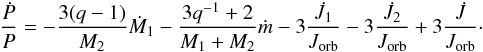 (2)The third and the fourth terms in Eqs. (1) and (2) induct the spin angular momentum contribution of each individual star by means of the consequential – advected – angular momentum transport, following the formalism of Gokhale et al. (2007); i.e.,
  and
and  . More particularly, in Eq. (1), j1 and j2 are the specific angular momenta of the matter leaving the donor and the matter arriving at the accretor at rates Ṁ1< 0 and Ṁ2> 0, respectively, whereas the opposite framework with Ṁ1> 0 and Ṁ2< 0 holds in Eq. (2).
Although the donor is not considered synchronized with the orbital motion in Gokhale et al. (2007), here it is assumed to be tidally locked, following the approach of many earlier studies (e.g., Nelemans et al. 2001; Marsh et al. 2004). Even for the gainer, tidal torques are disregarded from our approach owing to the wide range of the synchronization timescales, dictated by the friction mechanism and the intrinsic properties of the stellar outer envelopes (Zahn 1977, 1989; Zahn & Bouchet 1989; Tassoul & Tassoul 1992a,b).
In Algols, for instance, tides seem incapable of spinning down the gainer during the transfer process (Dervişoğlu et al. 2010; Deschamps et al. 2013), considering that radiative damping is the driving tidal dissipation mechanism for stars with a radiative envelope (Zahn 1977). By using the appropriate tidal torque and apsidal motion constants of Zahn (1975, see Table 1 of his work) for the gainer of IO UMa (M1 = 2.1 M⊙, e.g., Soydugan et al. 2013), for example, a long synchronization time of 9.69 × 10⁹ yr arises. In stars possessing a convective envelope, on the other hand, turbulent viscosity becomes the dominant tidal-braking process, a much more effective mechanism than the radiative dissipation (Zahn 1977). Considering the low-mass accretor of the system RY Aqr (M1 = 1.27 M⊙, e.g., Helt 1987), which has fractional radius (with respect to the orbital) similar to that of the gainer in IO UMa (~ 0.17), a timescale that is four orders of magnitude shorter, 5.23 × 10⁵ yr, is estimated. Tides may also play an important role in the spin rates of double white dwarfs and cataclysmic variables. Although the viscosity of degenerate matter suggests timescales on the order of 1015 yr, turbulent dissipation and the excitation of the non-radial modes are able to shorten the synchronization time in values even lower than 500 yr (see Marsh et al. 2004, and references therein). As a result, neglecting tidal coupling might affect our approach mostly when turbulent convection is the principal friction process, expected in late-type stars and, possibly, in degenerate components.
In both Eqs. (1) and (2), the fifth r.h.s. term represents the angular momentum lost by the system (at a rate  ), while Jorb accounts for the orbital angular momentum:
 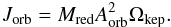 (3)In Eq. (3), Mred = M1M2/ (M1 + M2) is the reduced mass of the system, Aorb = G1/3(M1 + M2)1/3P2/3/ (2π)2/3 is the orbital radius, Ωkep = 2π/P is the Keplerian angular velocity, and G the gravitational constant.
The differential Eqs. (1) and (2) can be solved analytically for the orbital period function P(t) when the action of each individual physical process (or any combination) of our interest is given or even simulated. In consequence, if ϵ denotes a real-valued – continuous – measure of the orbital cycle (which also includes integer values when primary light minima are concerned, e.g., Gimenez & Garcia-Pelayo 1983; Borkovits et al. 2003), the orbital period as a function of time, P(t), is converted into the orbital cycle domain, P(ϵ), through the t = t(ϵ) transformation that emerges by solving for t the following equation:  (4)In this way, the function ΔT(ϵ) that practically represents the synthetic (theoretically anticipated) ETV diagram is eventually determined, supposing that the calculated times of minima are supplied by a linear ephemeris with initial minimum time T0 and reference period Pe. Indeed, as the P(t) function is given by Eqs. (1) or (2) along with its cycle transformed counterpart P(ϵ) (through Eq. (4)), then ΔT(ϵ) can be specified by solving the following differential equation (e.g., NKARL11):
 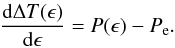 (5)All involved ordinary first-order differential equations (i.e., Eqs. (1)/(2), (4), and (5)) are solved under the initial conditions (ϵ,t,P(ϵ),ΔT(ϵ)) = (0,T0,Pe,0) that eventually provide the ΔT(ϵ) function. If, additionally, ε denotes the noise level of an ETV diagram, the critical number of epochs ϵmin, needed for the detection of a signal induced by a certain mechanism, is then made available by solving the equation,
  (6)which, alternatively, provides the number of epochs such that the signal-to-noise ratio equals one.
Similarly to NKARL11, the value of ε = 0.001 d is considered here as a typical noise level associated with photoelectric times of minima, ε = 0.03 d is adopted as a typical value associated with visual or patrol plates times of minima, while ε = 0.01 d serves as a pilot statistical noise level (i.e., for cases where the presence of migrating spots cannot be excluded, see also Kalimeris et al. 2002).
3. Examination of physical mechanisms
The implementation of the preceding methodology follows in four sections. In the first we examine the effects that MT through the L1 point (including those induced by a hot-spot emission) has on ETV diagrams, while the second section considers the effects of ML through the outer Lagrangian points L2 and L3. In the third section, we design non-conservative MT schemes that unveil the ETV diagram curvature based on the mass ratio of a system for a certain degree of conservation. Finally, in a fourth, the impact of AML via gravitational radiation in the O−C modulation, is examined.
3.1. Case I: mass exchange through the L1 point
A semi-detached configuration is attained as long as one of the two components of a binary system reaches the limiting surface of the Roche lobe. The MT process, also known as Roche lobe overflow (RLOF), is then realized through a critical (i.e., gravitationally neutral) point that coincides with the Lagrangian point L1 for a fully synchronized system (e.g., Kuiper 1941; Kopal 1956; Plavec 1958; Kruszewski 1963).
The inflowing matter may either hit the gainer directly (hereafter direct-impact mode), or it can orbit around the gainer, producing internal particle collisions due to intersecting trajectories. A gaseous ring is built in this way and eventually turns into an accretion disk owing to the effects of the gaseous material bulk viscosity (hereafter disk formation mode, e.g., Kruszewski 1967; Kříž 1971; Lubow & Shu 1975, 1976; Papaloizou & Pringle 1977; Lin & Papaloizou 1979; Shu & Lubow 1981). The latter occurs when the detached component has smaller radius than a critical value, Rmin = rminAorb, with rmin to be given as a function of the mass ratio of the system:  (7)when the donor is the more massive component, and
  (8)when the donor is the less massive component.
This approximation has emerged from the ballistic calculations of Lubow & Shu (1975, see Table 2 of their work) and is valid for 0.07 ≤ q ≤ 1 with accuracy close to 1% when the donor is the more massive component and better than 0.5% when the donor is the less massive component.
3.1.1. Mass transfer in the absence of an accretion disk
In the direct-impact MT mode, the flow stream coming from the donor hits the gainer and dissipates without creating an accretion disk when the radius of the gainer is much larger than the respective critical value Rmin (e.g., Kříž 1971; Lubow & Shu 1975). The stream strikes the gainer almost perpendicular to its surface and generates enough turbulence to keep the friction timescale short (Biermann & Hall 1973; Kaitchuck et al. 1985). As a result, tidal interaction seems efficient enough to keep both components in a strong coupling regime, canceling the angular momentum flows within the binary (e.g., Hut & Paczynski 1984; Verbunt & Rappaport 1988), i.e.  . The orbital angular momentum then remains invariable, and the period varies as a result of the mass redistribution between the two components.
In the fully conservative framework  , the relation given by Eqs. (1) or (2) is reduced to an ordinary first-order differential equation of the form,
  (9)where, when the donor is the more massive star, wL1 is given by
 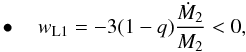 (10)while, when the donor is the less massive star, wL1 is given by
 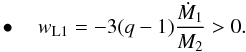 (11)Similar to NKARL11, the coefficient of proportionality between the rate at which period changes and the period itself, wL1, is considered constant since Ṁi terms are small enough to affect the absolute parameters of any of the components during the time windows covered even by the longest available ETV diagrams. Therefore, solution of Eq. (9) becomes trivial and under the initial condition (t,P(t)) = (T0,Pe) is written as
 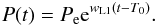 (12)Then, integration of Eq. (4) under the initial condition (ϵ,t) = (0,T0) yields
 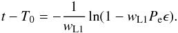 (13)As a result, through Eqs. (12) and (13), the orbital period P(ϵ) as a function of the continuous time variable ϵ is
 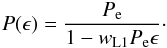 (14)Subsequently, integration of Eq. (5) under the initial condition (ϵ,ΔT(ϵ)) = (0,0) eventually gives the corresponding solution for the ΔT(ϵ) function:
  (15)Equation (15) implies that the curvature of the ΔT(ϵ) function, and subsequently the anticipated form of the respective ETV diagram, is determined by the sign of the constant wL1. In particular, when the donor is the more massive star (wL1< 0, see Eq. (10)), the orbital period decreases (see Eq. (9)) so the ΔT(ϵ) function is concave for any ϵ (see Eq. (11)). Likewise, when the donor is the less massive star (wL1> 0), the orbital period increases while the ΔT(ϵ) function is convex for any ϵ. Therefore, the foregoing analysis recovers the widely used procedure for estimating MT rates under conservative conditions in semi-detached and contact binaries (e.g., Kwee 1958; Huang 1963; Kruszewski 1964b).
Given the ΔT(ϵ) function, Eq. (6) is solved by a suitable Newton-Raphson numerical scheme (e.g., Press et al. 1992) in order to determine the minimum epoch ϵmin and the subsequent temporal intervals t(ϵmin) − T0 from Eq. (13). Our test case concerns a q = 0.5 semi-detached binary with a main-sequence secondary gainer of fractional radius r2 = R2/Aorb = 0.17 or a main-sequence primary gainer of fractional radius r1 = R1/Aorb = 0.25, keeping the secondary as massive as before. Results for several MT rates with a pilot noise level of ε = 0.01 d (in Eq. (6)) are given in Table 1, while for ε = 0.001 d and 0.03 d, the expected intervals are depicted in Fig. 1a. Similar computations were also made for various q values at Ṁ1 = 10-8 M⊙ yr-1 (see Fig. 1b), always taking into consideration that r2, r1 ≫ rmin should be valid. The temporal intervals are expected to be the same regardless of the component from which the mass begins to flow (given that |1 − q| remains constant) and that they do not depend on the reference period as long as Eq. (9) holds (see NKARL11).
Minimum time spans at ε = 0.01 d in absence of an accretion disk (conservative case).
 |
Fig. 1 Minimum time spans in a conservative era a) for several mass transfer rates when the mass ratio is fixed at q = 0.5 and b) for various mass ratios when the mass transfer rate is fixed at 10-8 M⊙ yr-1. Computations were performed both in the absence (circles) and in the presence of a transient disk around either the less massive (squares) or the more massive component (up triangles), for noise levels equal to 0.001 d (left vertical axis) and 0.03 d (right vertical axis). The dashed line in the right panel covers the range within which the critical value qcr ≈ 0.83 lies. (This figure is available in color in the electronic edition.) |
Because most of the available times of minima span slightly more than a century, a close inspection of Fig. 1 shows that under a low noise level of ε = 0.001 d, the signal of the conservative MT process without disk formation can be detected at rates Ṁi greater than 10-10 M⊙ yr-1, and mass ratios even close to unity. For higher noise levels, such as ε = 0.01 d or 0.03 d, the signal is rendered measurable only when Ṁi> 10-9 M⊙ yr-1 and q< 0.9 (see Table 1 and Fig. 1). The aforementioned ascertainments are in fairly good agreement with MT rates derived so far by traditional approaches for different binary types with at least one component filling its Roche lobe, ranging from 10-8 M⊙ yr-1 to 10-5 M⊙ yr-1 (e.g., Kaszás et al. 1998; Šimon 1999; Qian & Liu 2000; Qian 2002; Qian & Boonrucksar 2002; Qian et al. 2007, 2008; Manzoori 2008; Zasche et al. 2008; Zhu et al. 2009; Christopoulou et al. 2011).
3.1.2. Mass transfer in the presence of a transient accretion disk
Still in the direct-impact MT mode, the stream may be deflected by the Coriolis force before striking the gainer when its radius is marginally above the respective critical value Rmin (e.g., Kříž 1971; Lubow & Shu 1975). The stream hits the gainer tangentially to its surface, torquing the star near its limb and producing a thin ring that is gradually transformed into a quasi-stationary disk structure (Kaitchuck et al. 1985; Peters 1989; Richards & Albright 1999). The disk will be considered as transient (or low viscous) when the bulk viscosity is not efficient enough to return the proffered angular momentum to the orbit (we adopt the notation of Kaitchuck et al. 1985) or, equivalently, when it experiences a weak coupling regime with the donor. The advected angular momentum progressively accumulates in the disk and spins up the gainer, forcing the orbital angular momentum to decrease as a result of the conservative status (see, for instance, Packet 1981 for an excellent review on this topic).
In the present work, the specific angular momentum arriving at the accretor is parameterized in terms of the circularization radius (e.g., Biermann & Hall 1973; Flannery 1975; Warner 1978; Hut & Paczynski 1984; Verbunt & Rappaport 1988), i.e. the equivalent radius of a ring Rr = rrAorb in a circular Keplerian orbit around the gainer that has the same specific angular momentum as the transferred mass. Hence,  and
and  are the specific angular momenta accumulated by the accretor as secondary or primary, respectively, resulting in angular momentum gain at rate
  and
and  for each corresponding case.
Here, we provide an empirical relation for the fractional radius of the ring rr as a function of the mass ratio q, inferred from the results of the semi-analytical approach of Lubow & Shu (1975) for sufficiently low initial flow stream velocities at the L1 point (see Table 2 of their work):  (16)when the donor is the more massive component, and
  (17)when the donor is the less massive component.
This approximation is valid for 0.07 ≤ q ≤ 1, with the average relative error of rr being estimated close to 1% when the donor is the more massive component and less than 0.5% when the less massive. In the latter case, we also refer to the even more accurate relation of Verbunt & Rappaport (1988) when a wider mass ratio range is needed (i.e., for 0.001 ≤ q ≤ 1).
As far as the specific angular momentum leaving the donor is concerned, if RL = rLAorb is the (equivalent) radius of its Roche lobe, for the purposes of the present study we simply adopt  in Eq. (1) and
  in Eq. (2), following the suggestion of Gokhale et al. (2007) and recalling that the donor here is synchronized with the orbital velocity and fills its Roche lobe. As a consequence, its inertia offers an extra store of angular momentum, leaving the donor at a rate equal to
 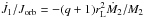 and
and 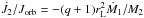 for each case, respectively, considering that Ṁ1 = − Ṁ2 in the conservative framework. The fractional Roche lobe radius rL is estimated via the empirical law of Eggleton (1983) with accuracy better than 1%, properly modified so that q ≤ 1 (e.g., Hilditch 2001):
 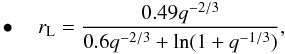 (18)when the donor is the more massive component, and
  (19)when the donor is the less massive component.
As a consequence, the relation, given by Eqs. (1) and (2), turns into an ordinary first-order differential equation identical to Eq. (9), Ṗ = wL1,rP, which can be solved for the orbital period P(t), by taking into account that, when the donor is the more massive star, the constant wL1,r is given by ![\begin{eqnarray} \label{equation:20} \bullet \quad w_{\mathrm{L1,r}}=-3\left[1-q+\sqrt{q(q+1)r_{\mathrm{r}}}-(q+1)r_{\mathrm{L}}^{2}\right]\frac{\dot{M}_{\mathrm{2}}}{M_{\mathrm{2}}}<0, \end{eqnarray}](/articles/aa/full_html/2015/03/aa23136-13/aa23136-13-eq162.png) (20)while, when the donor is the less massive star, wL1,r is given by
(20)while, when the donor is the less massive star, wL1,r is given by ![\begin{eqnarray} \label{equation:21} \bullet \quad w_{\mathrm{L1,r}}=-3\left[q-1+\sqrt{(q+1)r_{\mathrm{r}}}-(q+1)r_{\mathrm{L}}^{2}\right]\frac{\dot{M}_{\mathrm{1}}}{M_{\mathrm{2}}}\cdot \end{eqnarray}](/articles/aa/full_html/2015/03/aa23136-13/aa23136-13-eq163.png) (21)Since the presence of a transient disk drains orbital angular momentum, when the donor is the more massive component, the orbital period still decreases with respect to the no-disk case (wL1,r< 0, see Eq. (20)). However, the sign of wL1,r is not steady when the donor is the less massive star (see Eq. (21)), so the period varies according to the degree the viscosity of the transient disk facilitates the orbital AML. High viscosity values favor a strong gainer-disk-orbit coupling regime that returns most of the transferred angular momentum back to the orbit; i.e., wL1,r> 0 and Ṗ> 0, while low viscosity values favor a weak coupling regime that is inadequate for restraining the orbital AML; i.e., wL1,r< 0 and Ṗ< 0. The extra deposit of angular momentum stemming from the spin contribution of the donor proves to be too weak to inhibit the orbital shrinkage.
(21)Since the presence of a transient disk drains orbital angular momentum, when the donor is the more massive component, the orbital period still decreases with respect to the no-disk case (wL1,r< 0, see Eq. (20)). However, the sign of wL1,r is not steady when the donor is the less massive star (see Eq. (21)), so the period varies according to the degree the viscosity of the transient disk facilitates the orbital AML. High viscosity values favor a strong gainer-disk-orbit coupling regime that returns most of the transferred angular momentum back to the orbit; i.e., wL1,r> 0 and Ṗ> 0, while low viscosity values favor a weak coupling regime that is inadequate for restraining the orbital AML; i.e., wL1,r< 0 and Ṗ< 0. The extra deposit of angular momentum stemming from the spin contribution of the donor proves to be too weak to inhibit the orbital shrinkage.
In the simplified framework of Eqs. (16)−(19), the sign of wL1,r is determined solely by the mass ratio of the system q. In particular, the unique root at q = 0.83 of the term 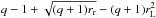 inside the brackets in Eq. (21), defines a critical value qcr of the mass ratio q so that
-
when q<qcr = 0.83, then Ṗ> 0 and ΔT(ϵ) is convex;
-
when q>qcr = 0.83, then Ṗ< 0 and ΔT(ϵ) is concave.
The detection of a critical value qcr for the mass ratio offers strong support to concave modulated ETV diagrams in high-mass-ratio, semi-detached binaries when the less massive component is the donor, contradicting the predictions of the conservative MT process in the absence of a disk.
Determination of the minimum time interval required in order to be the signal of the examined process observable in an ETV diagram initially concerns a q = 0.5 semi-detached binary with a main-sequence gainer of fractional radius r2 = R2/Aorb = 0.07 or r1 = R1/Aorb = 0.09 as the secondary or primary components, respectively. Were computed several MT rates for both the pilot noise level ε = 0.01 d (see Tables 2 and 3) and the more extreme cases of ε = 0.001 d and 0.03 d (see Fig. 1a). The same procedure was repeated for various q values at a steady MT rate of 10-8 M⊙ yr-1 (see Fig. 1b) by evaluating that the gainer’s fractional radius always lies between rmin and rr, quantities that are also presented in Tables 2 and 3.
Minimum time spans at ε = 0.01 d in the presence of a transient disk around the less massive component (conservative case).
Minimum time spans at ε = 0.01 d in the presence of a transient disk around the more massive component (conservative case).
Although the inferred intervals t(ϵmin) − T0 are found to be slightly different with respect to those in the absence of a disk when the donor is the primary component, they are severely broadened in the opposing framework, requiring MT rates enhanced by at least one order of magnitude (i.e., greater than 10-9 for ε = 0.001 d and 10-8 M⊙ yr-1 for ε = 0.03 d). Beside this, the existence of a critical mass ratio qcr ≈ 0.83, around which the period is expected to remain approximately invariable, makes detecting such a signal in an ETV diagram even harder. In practice, systems with mass ratio between 0.8 and 0.9 are expected to display no visible O−C variations with any of the adopted noise levels.
3.1.3. Mass transfer in the presence of a permanent accretion disk
In the disk formation MT mode, the stream misses completely the gainer when its radius is below the respective critical value Rmin (e.g., Kříž 1971; Lubow & Shu 1975). As a consequence, a rotating ring is formed that spreads out and is progressively transmuted into a stationary disk structure (e.g., Papaloizou & Pringle 1977; Lin & Papaloizou 1979). The disk will be considered as permanent (or high viscous) provided that the fluid’s material bulk viscosity is efficient enough to return the proffered angular momentum back to the orbit (once more, we adopt the notation of Kaitchuck et al. 1985) or, equivalently, when it experiences a strong coupling regime with the donor (e.g., Hut & Paczynski 1984; Verbunt & Rappaport 1988). However, material at the inner edge of the disk still has angular momentum that acts to spin up the accretor at the expense of the orbital angular momentum (e.g., Packet 1981; Marsh et al. 2004; Dervişoğlu et al. 2010; Deschamps et al. 2013).
The description of the period evolution of such systems does not differ at all from those systems that accommodate a transient disk, by simply replacing rr by r2 = R2/Aorb or r1 = R1/Aorb when the gainer is the less or the more massive star, respectively (Marsh et al. 2004). The minimum temporal intervals t(ϵmin) − T0 derived in the presence of a transient disk should be considered mostly as an upper limit (see Tables 2 and 3 and Fig. 1), while the results inferred in the absence of a disk should mostly be regarded as a lower limit (see Table 1 and Fig. 1), reflecting the case where r2 ≪ 1 or r1 ≪ 1 when the gainer is the secondary or the primary, respectively.
3.1.4. Mass and angular momentum loss through a hot-spot emission
When a semi-detached binary undergoes a MT phase, a hot spot is expected to be created in the area that the inflowing material impacts the mass-gaining component (whether an accretion disk is present or not, e.g., Kruszewski 1964a; Smak 1971; Warner & Nather 1971; Lubow & Shu 1975, 1976). As long as the radiative energy of such a hot spot, strengthened due to the limited accreted area (along with the rotational kinetic energy), surmounts the gravitational binding energy, the system is subject to a short non-conservative era, generally expected soon after the onset of the RLOF phase. It is proved that this condition is fulfilled provided that a critical MT rate has been reached (van Rensbergen et al. 2008). As a result, a hot spot can be a key factor in impelling a binary to a non-conservative phase.
Here, the AML process is parameterized in terms of the orbital specific angular momentum by adopting the formalism of Rappaport et al. (1982): 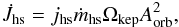 (22)where ṁhs< 0 denotes the ML rate during the non-conservative era and jhs the – dimensionless – specific angular momentum taken away from the orbit of the accreting star; i.e., jhs = (1/1 + q)2, if this is the secondary, and jhs = (q/ 1 + q)2, if this is the primary star (de Mink et al. 2007; Rensbergen et al. 2011). The AML term in Eqs. (1) and (2) is then equal to
  ṁhs/M2.
Attempting to isolate the ML and AML effects caused by the presence of a hot spot on the orbital evolution, we proceed by disregarding the MT term (i.e., Ṁi = 0), and the spin angular momentum of both components as well (i.e., ); in other words, we explore the impact that a fully liberal era (in which a hot spot emits all the incoming material) has on an ETV diagram morphology in the absence of a disk. The differential equation that governs the orbital evolution of the system, as derived from Eqs. (1) and (2), therefore has a similar form to Eq. (9), Ṗ = wL1,hsP, with the wL1,hs constant being given by the following relations: 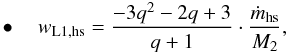 (23)when the donor is the more massive component, and
 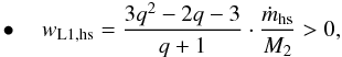 (24)when the donor is the less massive component.
Equations (23) and (24) make it clear that the prevalence of the driving mechanism (the ML process itself against the ML-induced torque through which the system loses angular momentum) depends directly on the mass ratio of the system. The sign investigation of wL1,hs in Eq. (23) shows that for binaries whose the donor is the primary star, the orbital period is expected to increase when q = qcr> 0.72, otherwise the period decreases. In contrast, in binaries whose donor is the secondary star, the orbital period is expected to increase regardless of the mass ratio q values. The above inference clearly shows that the AML effect hardly compensates for the ML process, resulting in an increasing period in most cases.
Determination of t(ϵmin) − T0 takes place following the standard procedure for the test cases examined in the direct-impact mode without a transient disk. The estimated temporal windows are quoted in Tables 4 and 5 for ε = 0.01 d, while they are graphically displayed in Fig. 2 for ε = 0.001 d and 0.03 d. Peering at the tabulated values, one notes that an O−C modulation is rendered observable for ML rates that exceed −10-9 M⊙ yr-1, barely favoring the case of the secondary star as the donor. Moreover, a non-conservative era due to a hot-spot emission from the secondary is expected to be measurable for almost any mass ratio except for a very narrow range between 0.7 and 0.8 (where qcrt0.72 lies).
Minimum time spans at ε = 0.01 d when a hot spot, located on the less massive component, emits all the incoming material (fully liberal case).
Minimum time spans at ε = 0.01 d when a hot spot, located on the more massive component, emits all the incoming material (fully liberal case).
By reducing the noise level at ε = 0.001 d, ML rates stronger than −10-10 M⊙ yr-1 are still detectable for a century, while no significant changes occur by worsening the noise contamination at ε = 0.03 d (Fig. 2a). However, by keeping the ML rate fixed at ṁhs = −10-8 M⊙ yr-1, the O−C variations are visible for ε = 0.001 d regardless of the mass ratio value, whereas a noise level increase at ε = 0.03 d limits the traceability of the examined mechanism only for very small mass ratios when the donor is expected to be the primary star (Fig. 2b).
3.2. Case II: mass and angular momentum loss through the L2/L3 points
In the course of a violent MT process in a semi-detached binary (e.g., in super-Eddington accretion flows), mass and angular momentum may be lost from the system either through the L2 or the L3 point when the donor is the more or the less massive component, respectively. These are the paths that matter can escape most easily from the gravitational field of the binary since it overcomes the lowest potential barrier, as a result requiring the lowest energy of all. The formation process and the observed features of a circumbinary envelope due to outflows from these two points have been confirmed or/and explored widely in literature (Kuiper 1941; Shu et al. 1979; Soberman et al. 1997; Spruit & Taam 2001; Taam & Spruit 2001; Chen et al. 2006; D’Souza et al. 2006; Motl et al. 2007; Sytov et al. 2007, 2009a,b; Zhilkin & Bisikalo 2009; Bisikalo 2010; Mennickent et al. 2010, 2012).
Here we adopt the AML parametrization proposed by Shu et al. (1979), which expresses the angular momentum taken away from the system via the L2 and L3 points in terms of the orbital specific angular momentum, similarly to the hot spot case. If ṁL2< 0, ṁL3< 0 defines the ML rate of the escaping matter from the L2 and L3 points with – dimensionless – specific angular momenta jL2, jL3, then  and
and  are estimated through Eq. (22) by properly substituting ṁhs and jhs for each corresponding case.
Intending to provide an efficient empirical relation for jL2 as a function of the mass ratio q, we employ the values of the semi-analytical ballistic model of Shu et al. (1979), as tabulated in Table 2 of their study. The values account for the terminal specific angular momentum (at very large distances from the system where the flow finally obtains its terminal kinematical characteristics), also taking the oblique impact angle the outflowing stream follows into account. In the absence of analytic calculations for jL3, we assume that matter leaves the system at the L3 point in a direction vertical to the line connecting the components (thus providing an upper AML limit); i.e.,  , with xL3 denoting the relative position of L3 in the Roche geometry coordinates system:
  (25)when ML and AML occur through L2, and
  (26)when ML and AML occur through L3.
This approximation is valid for 0.05 ≤ q ≤ 1 with accuracy better than 0.5% for both jL2 and jL3; however, jL3 represents the initial specific angular momentum (i.e., at L3), and a more reliable error close to 15% should be considered (as estimated by comparing the values of initial and terminal specific angular momentum for jL2, which are listed in Table 2 of Shu et al. 1979).
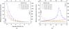 |
Fig. 2 Minimum time spans in a fully liberal era a) for several mass loss rates when the mass ratio is fixed at q = 0.5 and b) for various mass ratios when the mass loss rate is fixed at −10-8 M⊙ yr-1. Computations were performed considering that the transferred material is lost from the system through a hot-spot emission, located either on the less massive (squares) or the more massive component (circles), and via the L2 (up triangles) or the L3 point (down triangles), for noise levels equal to 0.001 d (left vertical axis) and 0.03 d (right vertical axis). The dashed line in the right panel covers the range within which the critical value qcr ≈ 0.72 lies. (This figure is available in color in the electronic edition.) |
Even after taking all assumptions mentioned in the hot spot case into consideration and specifying that the AML terms  and
and  in Eqs. (1) and (2) are equal to jL2(q + 1)ṁL2/M2 and jL3(q + 1)ṁL3/M2, respectively, the orbital evolution of the system is then still described by Eq. (9) by setting the wL2 constant in place of wL1 as
  (27)when ML and AML occur through L2, and
  (28)when ML and AML occur through L3.
It is noteworthy that the sign of the numerator appeared on the r.h.s. of Eqs. (27) and (28) is positive for any mass ratio q (since jL2, jL3> 1). Unlike the hot spot case, specific angular momentum is carried away from the system at a rather distant point (with respect to the center of mass), leading to markedly different AML rates and warranting period reduction (jhs< 1). As a result, the outer Lagrangian points L2 and L3 turn out to be routes through which the excess of matter, surviving the MT process, travels out of the system with prominent AML rates, ensuring orbital shrinkage.
To examine the measurability of the ML mechanism through the L2 and the L3 points, the standard methodology followed thus far is applied by retaining the binary parameters used in the absence of a disk case. Accurate values regarding the minimum intervals t(ϵmin) − T0 are given in Tables 6 and 7 for ε = 0.01 d, while they are graphically demonstrated in Fig. 2 for the two more noise levels of ε = 0.001 d and 0.03 d.
Minimum time spans at ε = 0.01 d when material, ejected from the more massive component, is carried away from the system through the L2 point (fully liberal case).
Careful inspection of the results reveals that the O−C differences are detectable as long as the ML rate from L2 exceeds −10-11 M⊙ yr-1 for ε = 0.001 d or −10-10 M⊙ yr-1 when the noise level takes higher values (i.e., ε = 0.01 or 0.03 d). However, the O−C residuals produced by ML via the L3 point need a modestly longer baseline of observations compared to the corresponding process via the L2 point. The mass ratio q proves to be a factor that hardly influences the temporal range t(ϵmin) − T0, lying in a few decades no matter what the adopted noise level is.
Minimum time spans at ε = 0.01 d when material, ejected from the less massive component, is carried away from the system through the L3 point (fully liberal case).
3.3. Case III: non-conservative mass transfer
We examine now what the combined effects of MT, ML, and AML processes might be in the modulation of an ETV diagram by distinguishing the case where the donor is the primary or the secondary component. Furthermore, we discern two subcases of each non-conservative MT case, addressing the general regime where a transient disk surrounds the gainer; the first concerns ML and AML realized by a hot-spot emission, while the second regards ML and AML from the L2/L3 point (non-captured mass from the gainer).
3.3.1. Critical mass ratios when the donor is the more massive star
If β ∈ [0,1] is the fraction of the MT rate gained by the accretor, then β = 1 represents the conservative case (where all the transferred mass is captured from the gainer), while β = 0 represents the fully liberal case (where all the transferred mass is rejected from the gainer).
As far as the donor is the more massive component and provided that Ṁ1 = − Ṁ2 + ṁ is valid, the MT rate captured by the secondary, Ṁ2, and the remaining fraction that evades the system, ṁ, can be written as  (29)and
  (30)In the first subcase (hot-spot-driven ML and AML from the secondary), we combine Eqs. (29) and (30) to express Ṁ1 and ṁhs as functions of the mass accretion rate Ṁ2. Then, Eq. (1) reduces into the following form:
 ![\begin{eqnarray} \label{equation:31} \frac{\dot{P}}{P}=\Bigg[-3(1-q)&-&3\sqrt{q(q+1)r_{\mathrm{r}}}+\frac{3}{\beta}\cdot(q+1)r_{\mathrm{L}}^{2}\nonumber \\&+&\frac{1-\beta}{\beta}\cdot\frac{3q^{2}+2q-3}{q+1}\Bigg]\frac{\dot{M}_{\mathrm{2}}}{M_{\mathrm{2}}}\cdot \end{eqnarray}](/articles/aa/full_html/2015/03/aa23136-13/aa23136-13-eq356.png) (31)Proceeding to the second subcase (ML and AML from L2), the rates Ṁ1 and ṁL2 are expressed as a function of Ṁ2 as well, and finally Eq. (1) takes the following form:
(31)Proceeding to the second subcase (ML and AML from L2), the rates Ṁ1 and ṁL2 are expressed as a function of Ṁ2 as well, and finally Eq. (1) takes the following form: ![\begin{eqnarray} \label{equation:32} \frac{\dot{P}}{P}=\Bigg[-3(1-q)&-&3\sqrt{q(q+1)r_{\mathrm{r}}}+\frac{3}{\beta}\cdot(q+1)r_{\mathrm{L}}^{2}\nonumber \\&-&\frac{1-\beta}{\beta}\cdot\frac{3j_{\mathrm{L2}}(q+1)^{2}-3q^{2}-2q}{q+1}\Bigg]\frac{\dot{M}_{\mathrm{2}}}{M_{\mathrm{2}}}\cdot \end{eqnarray}](/articles/aa/full_html/2015/03/aa23136-13/aa23136-13-eq357.png) (32)It is worth noting that on the r.h.s. of Eqs. (31) and (32), the expression within the brackets is a function of the mass ratio q alone. As a consequence, in the framework of our hypothesis set (and as long as β is treated as a free parameter), the mass ratio q becomes a crucial factor that modulates the variations (actually the monotonicity) of the period function P(t), as well as the geometrical form (actually the curvature) of the respective ETV diagram. The critical mass ratio values qcr can therefore arise after determining the roots of this expression, for any β, considering the direct MT mode either in the presence of a transient disk orbiting the secondary or in the absence of a disk. This can be achieved by calculating rr from Eq. (16) and rL from Eq. (18) in the former case and by setting rr = rL = 0 in the latter. Results for qcr are then presented in Table 8. Binary systems with mass ratio q greater than the listed qcr values will reveal an increasing period (and a convex ETV diagram), as long as the driving processes are those examined in the current section. New qcr values can emerge by substituting r2 for rr in the permanent disk formation mode.
(32)It is worth noting that on the r.h.s. of Eqs. (31) and (32), the expression within the brackets is a function of the mass ratio q alone. As a consequence, in the framework of our hypothesis set (and as long as β is treated as a free parameter), the mass ratio q becomes a crucial factor that modulates the variations (actually the monotonicity) of the period function P(t), as well as the geometrical form (actually the curvature) of the respective ETV diagram. The critical mass ratio values qcr can therefore arise after determining the roots of this expression, for any β, considering the direct MT mode either in the presence of a transient disk orbiting the secondary or in the absence of a disk. This can be achieved by calculating rr from Eq. (16) and rL from Eq. (18) in the former case and by setting rr = rL = 0 in the latter. Results for qcr are then presented in Table 8. Binary systems with mass ratio q greater than the listed qcr values will reveal an increasing period (and a convex ETV diagram), as long as the driving processes are those examined in the current section. New qcr values can emerge by substituting r2 for rr in the permanent disk formation mode.
Critical mass ratios qcr as a function of the degree of liberalism β when the donor is the more massive component (see text for details).
3.3.2. Critical mass ratios when the donor is the less massive star
As far as the donor is the less massive component and provided that Ṁ2 = −Ṁ1 + ṁ holds, the following relations are valid for the mass accretion and the ML rates, Ṁ1 and ṁ, respectively:  (33)and
 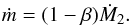 (34)In the first subcase (hot-spot-driven ML and AML from the primary), we combine Eqs. (33) and (34) to express Ṁ2 and ṁhs as a function of the mass accretion rate Ṁ1 and, subsequently, Eq. (2) is written as
 ![\begin{eqnarray} \label{equation:35} \frac{\dot{P}}{P}=\Bigg[-3(q-1)&-&3\sqrt{(q+1)r_{\mathrm{r}}}+\frac{3}{\beta}\cdot(q+1)r_{\mathrm{L}}^{2}\nonumber \\&-&\frac{1-\beta}{\beta}\cdot\frac{3q^{2}-2q-3}{q+1}\Bigg]\frac{\dot{M}_{\mathrm{1}}}{M_{\mathrm{2}}}\cdot \end{eqnarray}](/articles/aa/full_html/2015/03/aa23136-13/aa23136-13-eq365.png) (35)In the second subcase (ML and AML from L3), both the accretion and the ML rate, Ṁ2 and ṁL3 respectively, are written as a function of Ṁ1, modifying Eq. (2) as
(35)In the second subcase (ML and AML from L3), both the accretion and the ML rate, Ṁ2 and ṁL3 respectively, are written as a function of Ṁ1, modifying Eq. (2) as ![\begin{eqnarray} \label{equation:36} \frac{\dot{P}}{P}=\Bigg[-3(q-1)&-&3\sqrt{(q+1)r_{\mathrm{r}}}+\frac{3}{\beta}\cdot(q+1)r_{\mathrm{L}}^{2}\nonumber \\ &-&\frac{1-\beta}{\beta}\cdot\frac{3j_{\mathrm{L3}}(q+1)^{2}-2q-3}{q+1}\Bigg]\frac{\dot{M}_{\mathrm{1}}}{M_{\mathrm{2}}}\cdot \end{eqnarray}](/articles/aa/full_html/2015/03/aa23136-13/aa23136-13-eq366.png) (36)The numerical expression within the brackets on the r.h.s. of Eqs. (35) and (36) depends exclusively on the mass ratio q of the system. Critical mass ratio values qcr then emerge by determining the roots of this expression for different β values, considering a transient disk around the primary, with rr and rL being estimated via Eqs. (17) and (19), respectively. Accordingly, the qcr values in the absence of a disk were derived by posing rr = rL = 0. Results for qcr values are then given in Table 9. Systems with mass ratios q greater than the listed qcr values are expected to show a decreasing orbital period (and a concave ETV diagram). The same procedure can be applied by substituting r1 for rr to find the corresponding qcr values in the presence of a permanent disk.
(36)The numerical expression within the brackets on the r.h.s. of Eqs. (35) and (36) depends exclusively on the mass ratio q of the system. Critical mass ratio values qcr then emerge by determining the roots of this expression for different β values, considering a transient disk around the primary, with rr and rL being estimated via Eqs. (17) and (19), respectively. Accordingly, the qcr values in the absence of a disk were derived by posing rr = rL = 0. Results for qcr values are then given in Table 9. Systems with mass ratios q greater than the listed qcr values are expected to show a decreasing orbital period (and a concave ETV diagram). The same procedure can be applied by substituting r1 for rr to find the corresponding qcr values in the presence of a permanent disk.
Critical mass ratios qcr as a function of the degree of liberalism β when the donor is the less massive component (see text for details).
In Fig. 3, synthetic ETV diagrams have been constructed by means of Eqs. (15), (35), and (36) for a q = 0.4 semi-detached system with a primary gainer of r1 = 0.13 when the mass accretion rate is fixed at Ṁ1 = 10-8 M⊙ yr-1. The geometry of the anticipated ETV diagram for the same system is modulated according to the MT mode and the degree of the liberalism (i.e., the β value). Indeed, for the system RR Dra, which is suspected of accommodating a transient disk orbiting the primary star (Kaitchuck et al. 1985), a conservative MT rate close to 6 × 10⁻⁷ M⊙ yr-1 is derived, while a value of 3 × 10⁻⁷ M⊙ yr-1 is (under)estimated by the conventional approach (Zasche et al. 2008). Moreover, the observed period variations of X Tri could be ascribed to a non-conservative MT process with ML rates through L3 ranging from −2 × 10⁻⁸ to −6 × 10⁻⁸ M⊙ yr-1 (see also Nanouris et al. 2013), whereas the conservative approach fails to provide any reasonable explanation (Rovithis-Livaniou et al. 2000).
3.4. Case IV: Angular momentum loss through gravitational radiation
The last studied individual case concerns the effects of gravitational wave radiation (GWR), a physical mechanism that is highly suspected to drive binaries evolution with mainly degenerate components (e.g., Kramer et al. 2006; Antoniadis et al. 2013). In non-degenerate binaries, GWR seems to become a significant source of AML once binaries reach the contact phase (Webbink 1976).
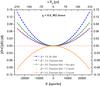 |
Fig. 3 Synthetic ETV diagrams for a q = 0.4 semi-detached system when the donor is the secondary star (step ≡ 1000 cycles). Squares and circles account for a conservative era (β = 1.0) either in the absence or in the presence of a transient disk, respectively. Upwardly pointing triangles (β = 0.9) account for a hot-spot-driven non-conservative era in the presence of a transient disk, while crosses (β = 0.7) and downwardly pointing triangles (β = 0.5) represent a non-conservative era where material escapes via the L3 point. (This figure is available in color in the electronic edition.) |
The rate at which a binary loses angular momentum because of the GWR mechanism is given by the well-known relation of Landau & Lifshitz (1962):  (37)where c is the speed of light in a vacuum. By ignoring MT and ML terms in Eqs. (1) and (2) and disregarding any other possible AML processes, the following differential equation is set and is solved for the orbital period P(t):
  (38)where the constant coefficient bg is given by the relation
  (39)The solution of Eq. (38) under the initial condition (t,P(t)) = (T0,Pe) is
 ![\begin{eqnarray} \label{equation:40} P(t)=\left[P_{\mathrm{e}}^{\frac{8}{3}}-\frac{8}{3}b_{\mathrm{g}}(t-T_{\mathrm{0}})\right]^{\frac{3}{8}}. \end{eqnarray}](/articles/aa/full_html/2015/03/aa23136-13/aa23136-13-eq387.png) (40)Then, integration of Eq. (4) under the initial condition (ϵ,t) = (0,T0) yields
(40)Then, integration of Eq. (4) under the initial condition (ϵ,t) = (0,T0) yields ![\begin{eqnarray} \label{equation:41} t-T_\mathrm{0}=\frac{3}{8b_{\mathrm{g}}}\left[P_{\mathrm{e}}^{\frac{8}{3}}-\left(P_{\mathrm{e}}^{\frac{5}{3}} -\frac{5}{3}b_{\mathrm{g}}\epsilon\right)^{\frac{8}{5}}\right]. \end{eqnarray}](/articles/aa/full_html/2015/03/aa23136-13/aa23136-13-eq388.png) (41)Hence, through Eqs. (40) and (41), the orbital period P(ϵ) as a function of the continuous time variable ϵ is
(41)Hence, through Eqs. (40) and (41), the orbital period P(ϵ) as a function of the continuous time variable ϵ is  (42)Integration of Eq. (5) under the initial condition (ϵ,ΔT(ϵ)) = (0,0) eventually gives the ΔT(ϵ) function
 ![\begin{eqnarray} \label{equation:43} \Delta T(\epsilon)=\frac{3}{8b_{\mathrm{g}}}\left[P_{\mathrm{e}}^{\frac{8}{3}}-\left(P_{\mathrm{e}}^{\frac{5}{3}} -\frac{5}{3}b_{\mathrm{g}}\epsilon\right)^{\frac{8}{5}}\right]-P_{\mathrm{e}}\epsilon, \end{eqnarray}](/articles/aa/full_html/2015/03/aa23136-13/aa23136-13-eq391.png) (43)which practically pictures the theoretically anticipated form of the ETV diagram under the action of GWR-AML, and is proved to be concave for any cycle ϵ, a result referring to the continuously decreasing orbital period function P(ϵ), expressed by Eq. (42).
(43)which practically pictures the theoretically anticipated form of the ETV diagram under the action of GWR-AML, and is proved to be concave for any cycle ϵ, a result referring to the continuously decreasing orbital period function P(ϵ), expressed by Eq. (42).
Minimum time spans at ε = 0.001 d and 0.01 d for several systems that lose angular momentum through gravitational radiation.
The traceability of a 1 + 1 M⊙, a 5 + 5 M⊙, and a 8 + 8 M⊙ system are then examined, all with Pe = 1 d. As seen in Table 10, even for a quite massive pair of 8 + 8 M⊙, it is almost impossible to observe any GWR-driven O−C variations, since at least 160 and 500 yr of dense monitoring are needed below noise levels equal to 0.001 and 0.01 d, respectively. In Table 10, we also tabulate the corresponding time intervals t(ϵmin) − T0 expected for the short-period contact binaries CC Com and W UMa (Pe< 0.4 d) and, beyond these, for the two massive binaries AH Cep and WR 20a (M1 + M2> 30 M⊙). Even for WR 20a, which is among the most massive binaries known to date (Bonanos et al. 2004), the GWR effects on its ETV diagram would only become detectable after 135 yr of accurate recorded times of minima.
An additional investigation is also performed to find out whether GWR-driven modulations are visible in a wide range of periods, varying from 0.1 to 1.0 d. All three hypothetical systems are explored, keeping in mind that a period threshold should exist for each case as a response to the contact configuration (Fig. 4). The critical limit of the orbital period Pcr was determined by considering radii of 3.6 R⊙ and 5.2 R⊙ for a 5 M⊙ and a 8 M⊙ dwarf star, respectively. Especially in the case of the 1 + 1 M⊙ system, the critical period Pcr was also determined considering that one member of the pair is a white dwarf with radius equal to 0.01 R⊙ (MS+WD).
A close inspection of Fig. 4 reveals that, as in the magnetic braking case (see NKARL11), the shorter the orbital period, the shorter the time required. Close to the period threshold of each examined system, slightly less than two centuries of observations are needed for producing measurable O−C variations. However, the MS+WD system seems to be an exceptional case that is likely to be highly detectable, demanding only five decades of monitoring at most. This finding mainly accommodates the group of eclipsing cataclysmic binaries with orbital periods of a few hours (see, e.g., Pilarčík et al. 2012, and references therein).
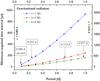 |
Fig. 4 Minimum time spans considering that gravitational radiation is the driving evolutionary process of a 1 + 1 M⊙ (squares), a 5 + 5 M⊙ (circles), and a 8 + 8 M⊙ system (up triangles) with various periods for noise levels equal to 0.001 d (left vertical axis) and 0.01 d (right vertical axis). The labels depict the period thresholds at which each system attains the contact configuration. (This figure is available in color in the electronic edition.) |
4. Discussion
We examined the orbital evolution and the associated synthetic ETV diagrams of binary systems that experience some of the most common manifestations of MT mechanisms in short, human life timescales. A complementary study was also carried out for GWR-induced modulations. The minimum range, required for the detectability of the ensuing O−C variations, was then estimated following the methodology introduced in Nanouris et al. (2011) for a variety of both physical and observational parameters where the procedure had been proved to be sensitive.
The conservative MT process was thoroughly investigated, and it was shown that for the direct-impact mode in the presence of a transient disk – which extracts large amounts of the orbital angular momentum – around the more massive component there is a critical mass ratio (qcr ≈ 0.83) above which the period turns out to decrease, contrary to those expectations that emerged by the conventional approach.
Different non-conservative MT modes were also examined by employing a parameter β to denote the degree of conservatism. Values of β close to zero account for violent non-conservative eras, while values close to unity account for highly conservative ones. Taking β as a free parameter in their hot-spot-driven evolutionary models, van Rensbergen et al. (2008) have shown that short non-conservative eras soon after an RLOF ignition may take place with a variable β, even reaching the value of β ~ 0.2. The present study revealed that in a non-conservative MT process induced by a hot-spot emission, AML is too weak to drive the orbital evolution, still allowing an increasing period even in strong but reasonable non-conservative eras (i.e., β ≤ 0.4), however only for a narrow range of high mass ratios (i.e., q ≥ 0.7) in systems where the donor is the primary star.
Instead, ML via the outer points L2 or L3 seems to be a strong AML process, capable of reducing the period at a very rapid pace. Sytov et al. (2007) have shown that the efficiency of accumulation in accretion disks of close binaries is not higher than 20−30% for typical values of turbulent viscosity, while it hardly reaches a rate of 50%, provided that the magnetic field is taken into consideration (Bisikalo 2010), impelling ML through L3 at significant amounts. We showed that the period is expected to decrease even during weak non-conservative eras through the L2 point, while when L3 is the libration point, it was revealed that there is always a critical mass ratio qcr above which the period is expected to decrease. The critical values qcr decrease as the degree of liberalism is progressively widened. Unlike the hot-spot emission, this allows a period reduction even for very low mass ratios (i.e., q ≤ 0.3) in systems where the donor is the secondary star.
The above findings prove that ML through the L3 point is a forceful candidate mechanism for interpreting the concave ETV diagrams that represent semi-detached systems with the less massive star to be the contact component (see, e.g., Yang & Wei 2009 for an updated catalog of binaries that display this peculiar behavior). Among them, AF Gem, TU Her, AT Peg, TY Peg, Z Per, Y Psc, and X Tri are systems with low mass ratios, and consequently, they are strongly suspected to undergo a non-conservative MT era, accompanied by ML through the L3 point at a significant rate. Recently, light curves of several early-type systems with an accretion disk have been analyzed using the new improved code of Djurašević et al. (2005, 2008) for estimating the physical disk parameters. Their analysis has indicated the presence of a bright spot, a region on the disk edge opposite (and close) to the L3 point, through which matter is expected to escape from the system. DL Cyg, β Lyr, AU Mon, V393 Sco, RY Sct, and DQ Vel are low mass ratio systems that could experience a non-conservative MT era.
It is noteworthy that the MT process is capable of driving the orbital evolution in the limited temporal range of ETV diagrams at rates similar to the wind-driven ML counterparts (NKARL11), implying that these two mechanisms might be strongly competitive (see also Erdem et al. 2005, 2007a,b). Consequently, ML through stellar winds should not be neglected in systems of semi-detached or contact configuration. Besides, the inferred critical mass ratios from the present analysis are expected to change considerably when this kind of ML is involved in our calculations. Evidently, the simplistic β − q schemes seem to be insufficient in describing the short orbital evolution of a binary in which MT is not the leading evolutionary mechanism. This may be consistent with the findings of Qian (2001), who has shown that a critical value close to qcr ≈ 0.40 appears to invert the monotonicity of the observed orbital evolution in contact binaries. However, this did not emerge clearly from the present study. The determination of the period monotonicity in the presence of numerous physical processes of a different nature, although feasible, is rather complicated and requires a more careful investigation.
The sufficiency of the commonly adopted parabolic representation of the long-term variations in ETV diagrams will be examined in a forthcoming paper through Taylorian expansions of the analytic ΔT(ϵ) expressions.
Acknowledgments
This project was funded by the State Scholarships Foundation of Greece (IKY) as part of the first author’s Ph.D. Thesis and financially supported by the Special Account for Research Grants (ELKE), No. 70/4/9702, of the National & Kapodistrian University of Athens, Greece. N.N. gratefully acknowledges them for their support. N.N. also acknowledges financial support under the “MAWFC” project. Project MAWFC is implemented under the “ARISTEIA II” action of the “OPERATIONAL PROGRAMME EDUCATION AND LIFELONG LEARNING”. The project is cofunded by the European Social Fund (ESF) and National Resources. We are thankful to the referee whose precious recommendations contributed to the improvement of both the methodology and the clarity of the manuscript. We would also like to thank Dr. A. Chiotellis for many valuable discussions and suggestions dealing with the orbital evolution of binary systems. This research has made use of SIMBAD database, operated at the CDS (Strasbourg, France) and NASA’s Astrophysics Data System Bibliographic Services.
References
- Antoniadis, J., Freire, P. C. C., Wex, N., et al. 2013, Science, 340, 448 [Google Scholar]
- Biermann, P., & Hall, D. S. 1973, A&A, 27, 249 [NASA ADS] [Google Scholar]
- Bisikalo, D. 2010, in Binaries – Key to Comprehension of the Universe, eds. A. Prša, & M. Zejda (San Francisco: ASP), ASP Conf. Ser., 435, 287 [Google Scholar]
- Bonanos, A. Z., Stanek, K. Z., Udalski, A., et al. 2004, ApJ, 611, 33 [Google Scholar]
- Borkovits, T., Érdi, B., Forgács-Dajka, E., & Kovács, T. 2003, A&A, 398, 1091 [NASA ADS] [CrossRef] [EDP Sciences] [Google Scholar]
- Burkholder, V., Massey, P., & Morrell, N. 1997, ApJ, 490, 328 [NASA ADS] [CrossRef] [Google Scholar]
- Chen, W.-C., Li, X.-D., & Qian, S.-B. 2006, ApJ, 649, 973 [NASA ADS] [CrossRef] [Google Scholar]
- Christopoulou, P.-E., Parageorgiou, A., & Chrysopoulos, I. 2011, AJ, 142, 99 [NASA ADS] [CrossRef] [Google Scholar]
- de Mink, S. E., Pols, O. R., & Hilditch, R. W. 2007, A&A, 467, 1181 [NASA ADS] [CrossRef] [EDP Sciences] [Google Scholar]
- Dervişoğlu, A., Tout, C. F., & Ibanoğlu, C. 2010, MNRAS, 406, 1071 [NASA ADS] [Google Scholar]
- Deschamps, R., Siess, L., Davis, P. J., & Jorissen, A. 2013, A&A, 557, A40 [NASA ADS] [CrossRef] [EDP Sciences] [Google Scholar]
- Djurašević, G., Rovithis-Livaniou, H., Rovithis, P., Borkovits, T., & Biró, I. B. 2005, New Astron., 10, 517 [NASA ADS] [CrossRef] [Google Scholar]
- Djurašević, G., Vince, I., & Atanacković, O. 2008, AJ, 136, 767 [NASA ADS] [CrossRef] [Google Scholar]
- Djurašević, G., Vince, I., Khruzina, T. S., & Rovithis-Livaniou, H. 2009, MNRAS, 396, 1553 [NASA ADS] [CrossRef] [Google Scholar]
- D’Souza, M. C. R., Motl, P. M., Tohline, J. E., & Frank, J. 2006, ApJ, 643, 381 [NASA ADS] [CrossRef] [Google Scholar]
- Eggleton, P. P. 1983, ApJ, 268, 368 [NASA ADS] [CrossRef] [Google Scholar]
- Erdem, A., Budding, E., Demircan, O., et al. 2005, Astron. Nachr., 326, 332 [Google Scholar]
- Erdem, A., Doğru, S. S., Bakiş, V., & Demircan, O. 2007a, Astron. Nachr., 328, 543 [NASA ADS] [CrossRef] [Google Scholar]
- Erdem, A., Soydugan, F., Doğru, S. S., et al. 2007b, New Astron, 12, 613 [Google Scholar]
- Flannery, B. P. 1975, MNRAS, 170, 325 [NASA ADS] [CrossRef] [Google Scholar]
- Gimenez, A., & Garcia-Pelayo, J. M. 1983, Ap&SS, 92, 203 [NASA ADS] [CrossRef] [Google Scholar]
- Giuricin, G., Mardirossian, F., & Mezzetti, M. 1984, A&A, 134, 365 [Google Scholar]
- Gokhale, V., Peng, X. M., & Frank, J. 2007, ApJ, 655, 1010 [NASA ADS] [CrossRef] [Google Scholar]
- Helt, B. E. 1987, A&A, 172, 155 [NASA ADS] [Google Scholar]
- Hilditch, R. W. 2001, An Introduction to Close Binary Stars (Cambridge: Cambridge Univ. Press) [Google Scholar]
- Hilditch, R. W., King, D. J., & McFarlane, T. M. 1988, MNRAS, 231, 341 [NASA ADS] [CrossRef] [Google Scholar]
- Huang, S.-S. 1963, ApJ, 138, 471 [NASA ADS] [CrossRef] [Google Scholar]
- Hut, P., & Paczynski, B. 1984, ApJ, 284, 675 [NASA ADS] [CrossRef] [Google Scholar]
- Kaitchuck, R. H., Honeycutt, R. K., & Schlegel, E. M. 1985, PASP, 97, 1178 [NASA ADS] [CrossRef] [Google Scholar]
- Kalimeris, A., & Rovithis-Livaniou, H. 2006, Ap&SS, 304, 113 [NASA ADS] [CrossRef] [Google Scholar]
- Kalimeris, A., Rovithis-Livaniou, H., & Rovithis, P. 2002, A&A, 387, 969 [NASA ADS] [CrossRef] [EDP Sciences] [Google Scholar]
- Kaszás, G., Vinkó, J., Szatmáry, K., et al. 1998, A&A, 331, 231 [NASA ADS] [Google Scholar]
- Koch, R. H., & Hrivnak, B. J. 1981, AJ, 86, 438 [NASA ADS] [CrossRef] [Google Scholar]
- Kopal, Z. 1956, Ann. Astrophys., 19, 298 [Google Scholar]
- Kramer, M., Stairs, I. H., Manchester, R. N., et al. 2006, Science, 314, 97 [NASA ADS] [CrossRef] [PubMed] [Google Scholar]
- Kříž, S. 1971, Bull. Astr. Inst. Czechosl., 22, 108 [Google Scholar]
- Kruszewski, A. 1963, Acta Astron., 13, 106 [NASA ADS] [Google Scholar]
- Kruszewski, A. 1964a, Acta Astron., 14, 231 [NASA ADS] [Google Scholar]
- Kruszewski, A. 1964b, Acta Astron., 14, 241 [NASA ADS] [Google Scholar]
- Kruszewski, A. 1967, Acta Astron., 17, 297 [NASA ADS] [Google Scholar]
- Kuiper, G. P. 1941, ApJ, 93, 133 [NASA ADS] [CrossRef] [Google Scholar]
- Kwee, K. K. 1958, Bull. Astron. Inst. Netherlands, 14, 131 [NASA ADS] [Google Scholar]
- Landau, L. D., & Lifshitz, E. M. 1962, The Classical Theory of Fields, 2nd edn. (Oxford: Pergamon) [Google Scholar]
- Lin, D. N. C., & Papaloizou, J. 1979, MNRAS, 186, 799 [NASA ADS] [CrossRef] [Google Scholar]
- Lubow, S. H., & Shu, F. H. 1975, ApJ, 198, 383 [NASA ADS] [CrossRef] [Google Scholar]
- Lubow, S. H., & Shu, F. H. 1976, ApJ, 207, 53 [Google Scholar]
- Manzoori, D. 2008, Ap&SS, 313, 339 [NASA ADS] [CrossRef] [Google Scholar]
- Marsh, T. R., Nelemans, G., & Steeghs, D. 2004, MNRAS, 350, 113 [NASA ADS] [CrossRef] [Google Scholar]
- Mennickent, R. E., Kołaczkowski, Z., Graczyk, D., & Ojeda, J. 2010, MNRAS, 405, 1947 [NASA ADS] [Google Scholar]
- Mennickent, R. E., Kołaczkowski, Z., Djurašević, G., et al. 2012, MNRAS, 427, 607 [NASA ADS] [CrossRef] [Google Scholar]
- Motl, P. M., Frank, J., Tohline, J. E., & D’Souza, M. C. R. 2007, ApJ, 670, 1314 [NASA ADS] [CrossRef] [Google Scholar]
- Nanouris, N., Kalimeris, A., Antonopoulou, E., & Rovithis-Livaniou, H. 2011, A&A, 535, A126 [NASA ADS] [CrossRef] [EDP Sciences] [Google Scholar]
- Nanouris, N., Kalimeris, A., Antonopoulou, E., & Rovithis-Livaniou, H. 2013, in Proc. 11th Conference of the Hellenic Astronomical Society, 39 [Google Scholar]
- Nelemans, G., Portegies Zwart, S. F., Verbunt, F., & Yungelson, L. R. 2001, A&A, 368, 939 [NASA ADS] [CrossRef] [EDP Sciences] [Google Scholar]
- Packet, W. 1981, A&A, 102, 17 [NASA ADS] [Google Scholar]
- Papaloizou, J., & Pringle, J. E. 1977, MNRAS, 181, 441 [NASA ADS] [CrossRef] [Google Scholar]
- Pilarčík, L., Wolf, M., Dubovský, P. A., Hornoch, K., & Kotková, L. 2012, A&A, 539, A153 [NASA ADS] [CrossRef] [EDP Sciences] [Google Scholar]
- Plavec, M. 1958, Mem. Soc. R. Sci. Liege, 20, 411 [Google Scholar]
- Press, W. H., Teukolsky, S. A., Vetterling, W. T., & Flannery, B. P. 1992, Numerical Recipes in Fortran 77, 2nd edn. (Cambridge: Cambridge Univ. Press) [Google Scholar]
- Peters, G. J. 1989, Space Sci. Rev., 50, 9 [NASA ADS] [CrossRef] [Google Scholar]
- Qian, S. 2001, MNRAS, 328, 635 [NASA ADS] [CrossRef] [Google Scholar]
- Qian, S. 2002, A&A, 384, 908 [NASA ADS] [CrossRef] [EDP Sciences] [Google Scholar]
- Qian, S., & Liu, Q. 2000, A&A, 355, 171 [NASA ADS] [Google Scholar]
- Qian, S.-B., & Boonrucksar, S. 2002, New Astron., 7, 435 [NASA ADS] [CrossRef] [Google Scholar]
- Qian, S.-B., Yuan, J.-Z., Liu, L., et al. 2007, MNRAS, 380, 1599 [NASA ADS] [CrossRef] [Google Scholar]
- Qian, S.-B., Liao, W.-P., & Fernández Lajús, E. 2008, ApJ, 687, 466 [NASA ADS] [CrossRef] [Google Scholar]
- Rappaport, S., Joss, P. C., & Webbink, R. F. 1982, ApJ, 254, 616 [NASA ADS] [CrossRef] [Google Scholar]
- Richards, M. T., & Albright, G. E. 1999, ApJS, 123, 537 [NASA ADS] [CrossRef] [Google Scholar]
- Rovithis-Livaniou, H., Kranidiotis, A. N., Rovithis, P., & Athanassiades, G. 2000, A&A, 354, 904 [NASA ADS] [Google Scholar]
- Shu, F. H., & Lubow, S. H. 1981, ARA&A, 19, 277 [NASA ADS] [CrossRef] [Google Scholar]
- Shu, F. H., Anderson, L., & Lubow, S. H. 1979, ApJ, 229, 223 [NASA ADS] [CrossRef] [Google Scholar]
- Šimon, V. 1999, A&AS, 134, 1 [NASA ADS] [CrossRef] [EDP Sciences] [Google Scholar]
- Smak, J. 1971, Acta Astron., 21, 15 [NASA ADS] [Google Scholar]
- Soberman, G. E., Phinney, E. S., & van den Heuvel, E. P. J. 1997, A&A, 327, 620 [NASA ADS] [Google Scholar]
- Soydugan, F., Soydugan, E., Kanvermez, Ç., & Liakos, A. 2013, MNRAS, 432, 3278 [NASA ADS] [CrossRef] [Google Scholar]
- Spruit, H. C., & Taam, R. E. 2001, ApJ, 548, 900 [NASA ADS] [CrossRef] [Google Scholar]
- Sterken, C. 2005, in The Light-Time Effect in Astrophysics (San Francisco: ASP), ASP Conf. Ser., 335, 3 [Google Scholar]
- Sytov, A. Yu., Kaigorodov, P. V., Bisikalo, D. V., Kuznetsov, O. A., & Boyarchuk, A. A. 2007, Astron. Rep., 51, 836 [Google Scholar]
- Sytov, A. Yu., Bisikalo, D. V., Kaigorodov, P. V., & Boyarchuk, A. A. 2009a, Astron. Rep., 53, 223 [NASA ADS] [CrossRef] [Google Scholar]
- Sytov, A. Yu., Bisikalo, D. V., Kaigorodov, P. V., & Boyarchuk, A. A. 2009b, Astron. Rep., 53, 428 [NASA ADS] [CrossRef] [Google Scholar]
- Taam, R. E., & Spruit, H. C. 2001, ApJ, 561, 329 [NASA ADS] [CrossRef] [Google Scholar]
- Tassoul, J.-L., & Tassoul, M. 1992a, ApJ, 395, 259 [NASA ADS] [CrossRef] [Google Scholar]
- Tassoul, M., & Tassoul, J.-L. 1992b, ApJ, 395, 604 [NASA ADS] [CrossRef] [Google Scholar]
- Tout, C. A., & Hall, D. S. 1991, MNRAS, 253, 9 [NASA ADS] [CrossRef] [Google Scholar]
- van Rensbergen, W., de Greve, J. P., de Loore, C., & Mennekens, N. 2008, A&A, 487, 1129 [NASA ADS] [CrossRef] [EDP Sciences] [Google Scholar]
- van Rensbergen, W., de Greve, J. P., Mennekens, N., Jansen, K., & de Loore, C. 2011, A&A, 528, A16 [NASA ADS] [CrossRef] [EDP Sciences] [Google Scholar]
- Verbunt, F., & Rappaport, S. 1988, ApJ, 332, 193 [NASA ADS] [CrossRef] [Google Scholar]
- Warner, B. 1978, Acta Astron., 28, 303 [NASA ADS] [Google Scholar]
- Warner, B., & Nather, R. E. 1971, MNRAS, 152, 219 [NASA ADS] [Google Scholar]
- Webbink, R. F. 1976, ApJ, 209, 829 [NASA ADS] [CrossRef] [Google Scholar]
- Yang, Y.-G., & Wei, J.-Y. 2009, AJ, 137, 226 [NASA ADS] [CrossRef] [Google Scholar]
- Zahn, J.-P. 1975, A&A, 41, 329 [NASA ADS] [Google Scholar]
- Zahn, J.-P. 1977, A&A, 57, 383 [NASA ADS] [Google Scholar]
- Zahn, J.-P. 1989, A&A, 220, 112 [NASA ADS] [Google Scholar]
- Zahn, J.-P., & Bouchet, L. 1989, A&A, 223, 112 [Google Scholar]
- Zasche, P., Liakos, A., Wolf, M., & Niarchos, P. 2008, New Astron, 13, 405 [NASA ADS] [CrossRef] [Google Scholar]
- Zhilkin, A. G., & Bisikalo, D. V. 2009, Astron. Rep., 53, 436 [NASA ADS] [CrossRef] [Google Scholar]
- Zhu, L.-Y., Qian, S.-B., Liao, W.-P., Zejda, M., & Mikulášek, Z. 2009, PASJ, 61, 529 [NASA ADS] [Google Scholar]
All Tables
Minimum time spans at ε = 0.01 d in absence of an accretion disk (conservative case).
Minimum time spans at ε = 0.01 d in the presence of a transient disk around the less massive component (conservative case).
Minimum time spans at ε = 0.01 d in the presence of a transient disk around the more massive component (conservative case).
Minimum time spans at ε = 0.01 d when a hot spot, located on the less massive component, emits all the incoming material (fully liberal case).
Minimum time spans at ε = 0.01 d when a hot spot, located on the more massive component, emits all the incoming material (fully liberal case).
Minimum time spans at ε = 0.01 d when material, ejected from the more massive component, is carried away from the system through the L2 point (fully liberal case).
Minimum time spans at ε = 0.01 d when material, ejected from the less massive component, is carried away from the system through the L3 point (fully liberal case).
Critical mass ratios qcr as a function of the degree of liberalism β when the donor is the more massive component (see text for details).
Critical mass ratios qcr as a function of the degree of liberalism β when the donor is the less massive component (see text for details).
Minimum time spans at ε = 0.001 d and 0.01 d for several systems that lose angular momentum through gravitational radiation.
All Figures
|
Fig. 1 Minimum time spans in a conservative era a) for several mass transfer rates when the mass ratio is fixed at q = 0.5 and b) for various mass ratios when the mass transfer rate is fixed at 10-8 M⊙ yr-1. Computations were performed both in the absence (circles) and in the presence of a transient disk around either the less massive (squares) or the more massive component (up triangles), for noise levels equal to 0.001 d (left vertical axis) and 0.03 d (right vertical axis). The dashed line in the right panel covers the range within which the critical value qcr ≈ 0.83 lies. (This figure is available in color in the electronic edition.) |
| In the text | |
|
Fig. 2 Minimum time spans in a fully liberal era a) for several mass loss rates when the mass ratio is fixed at q = 0.5 and b) for various mass ratios when the mass loss rate is fixed at −10-8 M⊙ yr-1. Computations were performed considering that the transferred material is lost from the system through a hot-spot emission, located either on the less massive (squares) or the more massive component (circles), and via the L2 (up triangles) or the L3 point (down triangles), for noise levels equal to 0.001 d (left vertical axis) and 0.03 d (right vertical axis). The dashed line in the right panel covers the range within which the critical value qcr ≈ 0.72 lies. (This figure is available in color in the electronic edition.) |
| In the text | |
|
Fig. 3 Synthetic ETV diagrams for a q = 0.4 semi-detached system when the donor is the secondary star (step ≡ 1000 cycles). Squares and circles account for a conservative era (β = 1.0) either in the absence or in the presence of a transient disk, respectively. Upwardly pointing triangles (β = 0.9) account for a hot-spot-driven non-conservative era in the presence of a transient disk, while crosses (β = 0.7) and downwardly pointing triangles (β = 0.5) represent a non-conservative era where material escapes via the L3 point. (This figure is available in color in the electronic edition.) |
| In the text | |
|
Fig. 4 Minimum time spans considering that gravitational radiation is the driving evolutionary process of a 1 + 1 M⊙ (squares), a 5 + 5 M⊙ (circles), and a 8 + 8 M⊙ system (up triangles) with various periods for noise levels equal to 0.001 d (left vertical axis) and 0.01 d (right vertical axis). The labels depict the period thresholds at which each system attains the contact configuration. (This figure is available in color in the electronic edition.) |
| In the text | |
Current usage metrics show cumulative count of Article Views (full-text article views including HTML views, PDF and ePub downloads, according to the available data) and Abstracts Views on Vision4Press platform.
Data correspond to usage on the plateform after 2015. The current usage metrics is available 48-96 hours after online publication and is updated daily on week days.
Initial download of the metrics may take a while.