| Issue |
A&A
Volume 574, February 2015
|
|
|---|---|---|
| Article Number | A43 | |
| Number of page(s) | 11 | |
| Section | Astrophysical processes | |
| DOI | https://doi.org/10.1051/0004-6361/201425027 | |
| Published online | 22 January 2015 | |
Reacceleration of electrons in supernova remnants
1 DESY, 15738 Zeuthen, Germany
e-mail: marpohl@uni-potsdam.de
2 Institute of Physics and Astronomy, University of Potsdam, 14476 Potsdam, Germany
Received: 19 September 2014
Accepted: 8 December 2014
Context. The radio spectra of many shell-type supernova remnants show deviations from those expected on theoretical grounds.
Aims. In this paper we determine the effect of stochastic reacceleration on the spectra of electrons in the GeV band and at lower energies, and we investigate whether reacceleration can explain the observed variation in radio spectral indices.
Methods. We explicitely calculated the momentum diffusion coefficient for 3 types of turbulence expected downstream of the forward shock: fast-mode waves, small-scale non-resonant modes, and large-scale modes arising from turbulent dynamo activity. After noting that low-energy particles are efficiently coupled to the quasi-thermal plasma, a simplified cosmic-ray transport equation can be formulated and is numerically solved.
Results. Only fast-mode waves can provide momentum diffusion fast enough to significantly modify the spectra of particles. Using a synchrotron emissivity that accurately reflects a highly turbulent magnetic field, we calculated the radio spectral index and find that soft spectra with index α ≲ − 0.6 can be maintained over more than 2 decades in radio frequency, even if the electrons experience reacceleration for only one acceleration time. A spectral hardening is possible but considerably more frequency-dependent. The spectral modification imposed by stochastic reacceleration downstream of the forward shock depends only weakly on the initial spectrum provided by, e.g., diffusive shock acceleration at the shock itself.
Key words: acceleration of particles / turbulence / cosmic rays / ISM: supernova remnants
© ESO, 2015
1. Introduction
The synchrotron spectra observed from shell-type supernova remnants (SNR) are conventionally interpreted as being produced by electrons that have been accelerated at the forward shock and possibly the reverse shock (Reynolds 2008) through a process known as diffusive shock acceleration (Bell 1978). The synchrotron spectra may extend to the hard X-ray band (Koyama et al. 1995), implying acceleration beyond 10 TeV electron energy and a potentially significant inverse-Compton emission component in the TeV band (Pohl 1996). Whereas the electron spectrum at very high energies is shaped by energy losses and the structure of the cosmic-ray precursor, GeV-band electrons should not be affected by losses and boundary effects. Their spectrum should reflect the canonical solution N(E) ∝ Es with s = 2 for strong shocks in monoatomic hydrogen gas. A slight softening of the spectra may arise from cosmic-ray feedback on the shock structure (Blandford & Eichler 1987) and a proper motion of the cosmic-ray scattering centers, such that the compression ratio of the scattering centers is lower than that of the gas.
The GeV-scale spectrum of electrons is probed with measurements of their synchrotron emission in the radio band. Green (2009) has compiled a catalog of 274 Galactic SNRs that includes information on the spectral index of their integrated radio emission. The values of the radio spectral index display a large scatter around a mean of α ≈ − 0.5 (Sν ∝ να, with α = (s − 1)/2), reaching in some cases α ≈ − 0.2 or α ≈ − 0.8. It is easy to see possible systematic uncertainties in the measurements. Contributions from a pulsar-wind nebula may harden the spectrum, but at least in cases with high-quality data over a wide frequency range, a lack of strong curvature in the spectrum would argue against that possibility. Likewise, confusion with H-II regions should be identifiable. Improper background subtraction should not be a problem for bright SNR like Cas A, which has a spectral index of α ≈ − 0.77.
It was realized early that stochastic acceleration might be a second relevant acceleration process (Drury 1983). Its efficiency was perceived to be low, and so few attempts have been made to explain the entire electron acceleration in SNR on this basis (Liu et al. 2008). If outward-moving Alfvén or fast-mode waves are resonantly excited in the shock precursor, their passage through the shock leads to a mixture of forward and backward moving waves (Vainio & Schlickeiser 1999). The Alfvén speed is low, though, and so is the momentum-diffusion coefficient calculated for scattering on them (e.g., Schlickeiser 2002). Fast-mode waves are a possible alternative, because their phase velocity is high in the downstream region (Liu et al. 2008). Non-resonant wave production typically yields linear waves with negligible phase velocity (e.g., Bell 2004), hence negligible efficacy for stochastic acceleration.
Here we re-examine the role of stochastic acceleration in SNR. It has been realized in recent years that non-resonant small-scale instabilities operating upstream in their non-linear phase impose substantial plasma turbulence that will foster second-order Fermi acceleration (Stroman et al. 2009). Secondary instabilities arise, for example by shock rippling, which leads to turbulent magnetic-field amplification downstream of the shock (Giacalone & Jokipii 2007; Mizuno et al. 2011; Inoue et al. 2011; Guo et al. 2012; Fraschetti 2013), along with turbulent motions that should eventually be in energy equipartition with the turbulent magnetic field (Mizuno et al. 2014). Both on small and on large scales we therefore expect some second-order Fermi acceleration to operate behind the outer shocks of SNRs. The inevitable decay of the turbulence will not only impose a spatial dependence on the acceleration rate, it will also have an impact on the synchrotron emissivity (Pohl et al. 2005). In fact, numerical modeling of particle motion in generalized magneto-hydrodynamic (MHD) turbulence suggests that for parameters typical of young SNRs a GeV-scale particle can experience acceleration on a time scale of ~100 years (Fatuzzo & Melia 2014, their experiment 9). Stochastic acceleration may thus act as a secondary re-acceleration process downstream of SNR shocks that slightly modifies the particle spectrum produced at the shock by diffusive shock acceleration. This is in contrast to some models of flares that posit an initial stochastic acceleration followed by a second stage of shock acceleration (Petrosian 2012).
In this paper we attempt an estimate of the re-acceleration rate for three types of turbulence: fast-mode waves as already discussed by Liu et al. (2008), Bell’s non-resonant instability, and large-scale MHD turbulence arising from shock rippling through dynamo processes. Having established the efficiency, energy dependence, and spatial decay scale of the momentum diffusion coefficient, we compute its effect on the differential number density of electrons between the forward shock and the contact discontinuity. We conclude with a discussion of the expected radio spectra of SNRs.
2. Estimating the rate of diffusive reacceleration
Before we discuss reacceleration rates in detail, it is important to recall that the downstream region of the forward shocks of young SNRs is not a low-β environment. The flow is subsonic by definition, whereas the Alfvén speed increases only with the shock compression. It has become popular to posit a high Alfvén velocity of a few hundred kilometers per second in the upstream region, which leads to softer particle spectra that fit better to observations. This benefit comes at the expense of reducing the Alfvénic Mach number of the forward shock to MA ≲ 10, rendering the magnetic field dynamically important (Caprioli et al. 2008) and an efficient energy sink.
2.1. Fast-mode waves
The fastest waves in the downstream region should be fast-mode waves whose phase velocity is the sound speed, vfm = cs ≃ 1000 km s-1. Particles can interact with fast-mode waves through transit-time damping (TTD), a process that does not have specific resonance scales. One consequence is that thermal particles will efficiently damp all waves except those that propagate parallel or perpendicular to the local magnetic field (Quataert 1998). The damping rate of waves with propagation angle θk to the large-scale magnetic field is of the order (Liu et al. 2008) ![\begin{eqnarray} &&\Lambda_\mathrm{d,fm}\approx \frac{2\pi\,c_\mathrm{s}\,\sin^2\theta_k}{\lambda\,\vert\cos\theta_k\vert}\ \nonumber \\ &&\times \left( \exp\left[-\frac{1}{\cos^2\theta_k}\right]+\sqrt{\frac{m_{\rm e}\,T_{\rm e}}{m_{\rm p}\,T_{\rm p}}}\,\exp\left[-\frac{m_{\rm e}\,T_{\rm p}}{m_{\rm p}\,T_{\rm e}\,\cos^2\theta_k}\right]\right) \ . \label{eq:1.1} \end{eqnarray}](/articles/aa/full_html/2015/02/aa25027-14/aa25027-14-eq16.png) (1)In the immediate postshock region of young SNRs the electron temperature, Te, is considerably lower than that of protons. In fact,
(1)In the immediate postshock region of young SNRs the electron temperature, Te, is considerably lower than that of protons. In fact,  and Te ≈ 0.01 Tp for shock speeds, vsh, around 4000 km s-1 (Ghavamian et al. 2007; van Adelsberg et al. 2008). The prefactor of the second exponential in Eq. (1) is therefore of the order 2 × 10⁻³, and the argument of the second exponential is approximately 1/(20 cos2θk) An estimate of the time scale of cascading is (Cho & Lazarian 2002)
  (2)where V is the amplitude of velocity fluctuations at the injection scale, λmax. We see that the entire spectrum of fast-mode waves will be anisotropic. Setting Λd,fmτc,fm = 1 gives the angle-dependent wavelength, λc, down to which the fast-mode turbulence can cascade.
The fast-mode turbulence can be expected to follow a 3D-spectrum (Cho & Lazarian 2002)  (3)where Θ is a step function and
  (4)with Ufm denoting the kinetic energy density in fast-mode waves and λmax is their driving scale. This spectrum refers to the magnetic fluctuations only, which are known to be weaker in energy density than the velocity fluctuations, and so the plasma beta appears in the denominator.
We calculate the momentum diffusion coefficient for an isotropic distribution of electrons as (Lynn et al. 2014)  (5)where ⊥ and ∥ refer to projections perpendicular and parallel to the local mean magnetic field, B0, and μ = cosθ reflects the pitch angle relative to it. The resonance function R(k,Ωk) includes the effects of orbit perturbations and can be written as (Yan & Lazarian 2008)
 ![\begin{eqnarray} R(k,\Omega_k)&=&\frac{1}{\sqrt{\pi}\,\vert \epsilon\,k_\parallel\,v_\perp\vert}\, \exp\left[-\frac{(k_\parallel\,v_\parallel-k\,c_{\rm s})^2}{\epsilon^2\,k_\parallel^2\,v_\perp^2}\right]\nonumber \\ &=& \frac{1}{\sqrt{\pi}\,\epsilon\,k\,c\,\vert \mu_k\vert\,\sqrt{1-\mu^2}}\, \exp\left[-\frac{(\mu-\frac{c_{\rm s}}{\mu_k\,c})^2}{\epsilon^2\,(1-\mu^2)}\right], \label{eq:1.7} \end{eqnarray}](/articles/aa/full_html/2015/02/aa25027-14/aa25027-14-eq38.png) (6)where μk = k∥/k and
(6)where μk = k∥/k and  involves the large-scale fluctuations in the magnetic field parallel to the mean field and should be of the order unity in the highly perturbed environment immediately downstream of a SNR forward shock.
Inserting Eqs. (3) and (6) into (5) we find ![\begin{eqnarray} D_{\rm p}&=&\frac{\sqrt{\pi}\,p^2\,c\,U_\mathrm{fm}}{8\,\epsilon\,B_0^2\,\beta\,\sqrt{\lambda_\mathrm{max}}}\, \int {\rm d}\mu\ \left(1-\mu^2\right)^{3/2}\nonumber \\[1.62mm] &&\times \int {\rm d}\mu_k\ \frac{\vert \mu_k\vert}{\sqrt{\lambda_{\rm c}}}\, \exp\left[-\frac{(\mu-\frac{c_{\rm s}}{\mu_k\,c})^2}{\epsilon^2\,(1-\mu^2)}\right]\cdot \label{eq:1.8} \end{eqnarray}](/articles/aa/full_html/2015/02/aa25027-14/aa25027-14-eq41.png) (7)We solve Eq. (7) separately for parallel and perpendicular waves in the Appendices A.1 and A.2, respectively. We cannot confirm the finding of Liu et al. (2008) who argue that the parallel modes are the most efficient accelerators of electrons. In fact, the perpendicular modes give a momentum diffusion coefficient that is somewhat larger than that of parallel modes.
(7)We solve Eq. (7) separately for parallel and perpendicular waves in the Appendices A.1 and A.2, respectively. We cannot confirm the finding of Liu et al. (2008) who argue that the parallel modes are the most efficient accelerators of electrons. In fact, the perpendicular modes give a momentum diffusion coefficient that is somewhat larger than that of parallel modes.
From Eq. (A.10) we find the acceleration time as 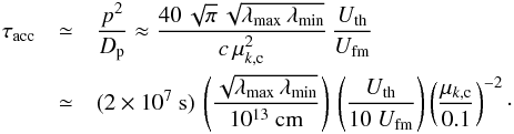 (8)This estimate for the time scale of stochastic acceleration is independent of momentum. It does rely on the isotropy of the particle distribution function, though. Calculating the isotropization time scale is beyond the scope of this paper, but a remark may be in order. Usually, isotropization becomes slower at high particle energies, and therefore Eq. (8) should be realistic only for low-energy particles with energy E ≲ 1 GeV.
Reaccelerating energetic particles is another damping process for fast-mode turbulence that we have not yet considered. Let us now consider a not too narrow range in k of the wave spectrum around wavelength λ. The wave energy density at that wavelength, and the acceleration time provided by it, are 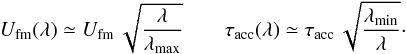 (9)Taking the acceleration time independent of energy as in Eq. (8), we find the energy transfer rate from turbulence to particles as
 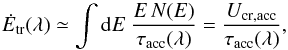 (10)where Ucr,acc denotes the energy density in cosmic rays that experience acceleration. We noted before that very-high-energy particles will probably not isotropize fast enough for our estimate of the acceleration time to be valid. The energy transfer, Ėtr(λ), reduces the energy density in fast-mode waves, Ufm(λ) on a time scale
 ![\begin{eqnarray} \tau_\mathrm{d,cr}(\lambda)&\simeq& \frac{U_\mathrm{fm}(\lambda)}{\dot E_\mathrm{tr}(\lambda)}\simeq \frac{U_\mathrm{fm}(\lambda)}{U_\mathrm{cr,acc}}\,\tau_\mathrm{acc}(\lambda) \nonumber \\[1.2mm] &\simeq& \frac{U_\mathrm{fm}}{U_\mathrm{cr,acc}}\,\tau_\mathrm{acc}\,\frac{\lambda}{\sqrt{\lambda_\mathrm{max}\,\lambda_\mathrm{min}}}\nonumber \\ &\simeq& \frac{U_\mathrm{th}}{U_\mathrm{cr,acc}}\,\frac{40\,\sqrt{\pi}\,\lambda}{c\,\mu_{k,{\rm c}}^2}\cdot \label{eq:1.9b} \end{eqnarray}](/articles/aa/full_html/2015/02/aa25027-14/aa25027-14-eq51.png) (11)The cosmic-ray induced damping of the waves must be slower than cascading, otherwise the fast-mode cascade would terminate. Comparing Eqs. (11) and (2) we find
(11)The cosmic-ray induced damping of the waves must be slower than cascading, otherwise the fast-mode cascade would terminate. Comparing Eqs. (11) and (2) we find 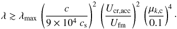 (12)Combined, Eqs. (11) and (12) illustrate conditions that must be met for stochastic reacceleration to be operational in the postshock region of SNR.
-
1.
There should not be less energy density in fast-mode waves thanin the part of the cosmic-ray spectrum in which re-acceleration isefficient.
-
2.
Unless we have much more energy in fast-mode turbulence than in energetic particles undergoing stochastic acceleration, cascading is quenched by TTD interaction with cosmic rays. Consequently, our estimate of the acceleration time scale in Eq. (8) is optimistic.
-
3.
Inserting the wavelength limit (Eq. (12)) as λmin into the expression (Eq. (8)) we find as more realistic, revised estimate of the acceleration time scale
![\begin{eqnarray} \tau_{\rm acc,rev} &\simeq& \frac{\lambda_{\rm max}}{4\pi\,c_{\rm s}}\, \frac{U_\mathrm{th}\,U_\mathrm{cr,acc}}{U_\mathrm{fm}^2} \\[1.2mm] &\simeq& (8 \!\times\! 10^7~{\rm s})\, \left(\frac{\lambda_\mathrm{max}}{10^{16}\,{\rm cm}}\right)\, \left(\frac{c_\mathrm{s}}{10^3\,{\rm km\,s^{-1}}}\right)^{-1}\,\frac{U_\mathrm{th}\,U_{\rm cr,acc}}{10~U_\mathrm{fm}^2}\cdot \nonumber \label{eq:1.9e} \end{eqnarray}](/articles/aa/full_html/2015/02/aa25027-14/aa25027-14-eq54.png) (13)The true acceleration time is thus a few years, and stochastic reacceleration will operate for only a few acceleration times.
(13)The true acceleration time is thus a few years, and stochastic reacceleration will operate for only a few acceleration times. -
4.
As the turbulence is driven at the shock and then advects downstream, we must expect that strong fast-mode turbulence exists only in a thin layer of a few λmax in thickness.
2.2. Small-scale non-resonant modes
Current-driven instabilities can lead to aperiodic small-scale turbulence (Winske & Leroy 1984), that include parallel (Bell 2004) and oblique modes (Malovichko et al. 2014). In conditions typical for the cosmic-ray precursors of the forward shocks of young SNR, the instability may operate for only a few growth times (Niemiec et al. 2008), unless the remnant expands into a high-density environment, in which case, however, one has to consider ion-neutral collisions, which can reduce the growth of the instability (Reville et al. 2007).
The saturation level of small-scale non-resonant modes is not well known. Estimates based on the shrinking of the driving particles’ Larmor radius lead to high saturation levels of a few hundred μG (Zirakashvili et al. 2008; Pelletier et al. 2006). A significant backreaction, however, is a reduction in streaming velocity and hence a diminishing of the streaming anisotropy, that leads to a lower saturation level and only moderately amplified magnetic field (Luo & Melrose 2009). Another non-linear side effect is turbulent motion (Stroman et al. 2009) which will add to the large-scale MHD turbulence discussed in the next subsection.
Relevant for us is that the modes have a very low real frequency, at least in the linear stage, and so we can describe them with reasonable accuracy in the magnetostatic approximation. They are excited on scales well below the Larmor radius of the driving particles. If we place the high-energy cut off in the particle spectra spectrum at 100 TeV and assume a magnetic-field strength of 10 μG, then the largest scale would be ~1016 cm. Particles of lower energies excite modes of smaller wavelength and, depending on the cosmic-ray spectrum, may be actually more efficient in driving small-scale turbulence than are the few particles at the highest energy that carry very little current. Gamma-ray observation of young SNR indicate relatively soft particle spectra, and so a more realistic estimate of the length scale of maximum intensity would be Lmax ≈ (1014 − 1015) cm. What turbulence spectrum is eventually established is a difficult question. Behind the shock little, if any, driving will transpire, and the spectrum is determined by cascading and damping until the energy reservoir at Lmax is drained.
Shalchi et al. (2009) have developed a second-order non-linear theory of wave-particle interaction that for an assumed spectrum ![\begin{equation} I_k \propto \frac{|k\,L_\mathrm{max}|^q}{\left[1+(k\,L_\mathrm{max})^2\right]^{(s+q)/2}} \label{eq:2.1} \end{equation}](/articles/aa/full_html/2015/02/aa25027-14/aa25027-14-eq60.png) (14)of strong magnetosonic slab turbulence yields for the momentum diffusion coefficient of relativistic particles with small Larmor radius, rL, (Shalchi 2012)
(14)of strong magnetosonic slab turbulence yields for the momentum diffusion coefficient of relativistic particles with small Larmor radius, rL, (Shalchi 2012) 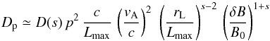 (15)where
 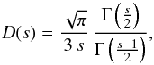 (16)δB is the turbulent field amplitude integrated over the entire turbulence spectrum 14, and vA is the Alfvén velocity. The diffusion coefficient would fall off steeply once rL ≳ rL,max where rL,max = LmaxB0/δB. The expression will certainly become inaccurate in the presence of other turbulence on larger scales, but it may still serve as an approximation.
The cascading behavior is likewise not well known. A generic Kolmogorov-type estimate (Ptuskin & Zirakashvili 2003) would suggest that the intensity at the largest scales decays on a time scale 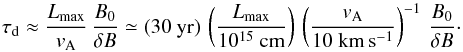 (17)The ratio of available time (Eq. (17)) to the acceleration time p2/Dp can be expressed with a step function Θ to mark the range of applicability of Eq. (15),
 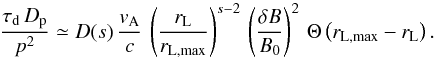 (18)It is typically small, unless vA is very large in the downstream region.
2.3. Large-scale MHD turbulence
The acceleration provided by moving magnetic-field structures is essentially a classical Fermi process. If scatterers move with random velocity vs and the frequency of collision with these structures is ω, then the momentum diffusion coefficient is (e.g. Lynn et al. 2013) 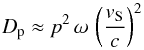 (19)Fraschetti (2013) estimates that the magnetic-field amplification factor is determined by the Field length (Inoue et al. 2006), LF, and the radius of curvature, RC, of the shock ripples,
  (20)where MA is the Alfvénic Mach number and θ is the typical angle between the local and the average shock normal. The radius of curvature, RC, can be related to the length scales of upstream density fluctuations, Lρ, as
  (21)Inserting numbers appropriate for young SNR one easily finds amplification factors of a thousand or more, because the size of upstream clouds, Lρ, is typically larger than the thickness of their interface to the dilute medium, LF. Inoue et al. (2012) have performed 3D-MHD simulations with MA ≃ 250 and find amplification factors considerably less than suggested by Eq. (21): the maximum field strength is about a factor 200 higher than the initial field, and the average field strength is amplified by approximately a factor 5. Similar results have been obtained in 2D-MHD simulations (Mizuno et al. 2011, 2014).
Turbulence spectra are usually difficult to extract on account of the limited spectral range of MHD simulations. Published simulations agree that velocity perturbations approximately follow a Kolmogorov scaling whereas the spectrum of magnetic perturbations is considerably flatter than that, possibly because the dynamo process has not saturated on large scales. The correlation properties between magnetic and velocity perturbations in the simulations of Mizuno et al. (2014) suggest that we may treat the turbulence structures as magnetic clouds of amplitude Bk moving with random velocity vk. The scattering rate is then determined by the time needed to propagate between clouds, either ballistically or through diffusion with mean free path λmfp, 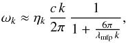 (22)where ηk is the efficiency of the process that is of the order unity only if the particles are indeed reflected upon passage through the magnetic structure, thus requiring
  (23)where the Larmor radius, rL, is to calculated using Brms. Hence, our estimate for ηk is
 ![\begin{equation} \eta_k\approx \left[1+\left(\frac{B_\mathrm{rms}\,r_\mathrm{L}}{B_k\,\lambda}\right)^2\right]^{-1}=\left[1+\left(\frac{B_\mathrm{rms}\,r_\mathrm{L}\,k}{2\pi\,B_k}\right)^2\right]^{-1}\cdot \label{eq:3.6} \end{equation}](/articles/aa/full_html/2015/02/aa25027-14/aa25027-14-eq89.png) (24)The momentum diffusion coefficient (Eq. (19)) is then determined through convolution with the turbulence spectrum,
(24)The momentum diffusion coefficient (Eq. (19)) is then determined through convolution with the turbulence spectrum,  (25)The single-cloud values of magnetic-field strength and velocity need to be replaced with integrals over the Fourier power spectrum, and hence we replace
  . Using Kolmogorov scaling for both velocity and magnetic perturbations,
  (26)one finds that the integrand in Eq. (25) has a sharp maximum at
  (27)The decay of the turbulence therefore affects the momentum diffusion coefficient in an easily tractable way: We need only consider the decay length at kmax. The integral 25 yields
  (28)If the spatial diffusion follows Bohm scaling (λmfp ≈ rL), then the acceleration time is independent of momentum.
Simulations suggest that the velocity fluctuations reach a few per cent of the shock speed, vrms ≃ vsh/ 20 (Mizuno et al. 2014). Inserting that in Eq. (28) we find for the acceleration time 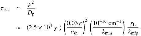 (29)This is much longer than the evolutionary time scales of SNR, unless kmin is very small. Type-Ia supernovae expand into the interstellar medium, in which a significant part of the high-density clouds arise from the thermal instability, and so the Field length, LF ≈ 1016 cm, sets the scale for kmin, thus rendering re-acceleration ignorable. Core-collapse supernovae, on the other hand, expand into the wind zone of their progenitors, which is essentially a collection of clumps of material that are radiatively driven outward (Lucy & White 1980) that can survive out to at least 1000 stellar radii (Runacres & Owocki 2002). Spectroscopic evidence for clumping has been presented in Lépine & Moffat (1999, 2008); Prinja & Massa (2010) with clumps sizes ranging up to approximately one stellar radius (Oskinova et al. 2007). In that case kmin ≈ 10-13 cm-1 and the acceleration time is only 20 years or so. The time available is limited by the forward shock of the proto-SNR leaving the region of significant clumping, and we find that clumps need to survive out to more than 104 stellar radii to permit a significant spectral distortion.
3. Calculation of electron spectra
The spatial transport of relativistic electrons behind the forward shock of SNR is provided by both advection and diffusion. We concern ourselves with GeV-scale electrons whose spatial-diffusion coefficient is most likely very small inside SNR. If we scale diffusion to the Bohm limit in a 100 μG magnetic field, 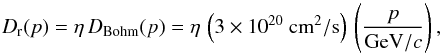 (30)then the typical displacement of an electron in a time period δt is
 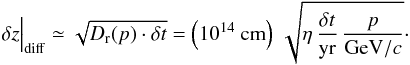 (31)In the same time period, advection in the downstream flow with typical speed vadv ≃ v8 (1000 km s-1) yields a displacement
 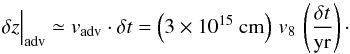 (32)For very small time periods and displacements from the forward shock,
 ![\begin{eqnarray} \delta t&\lesssim& (3\times 10^4~\mathrm{s})\,\frac{\eta}{v_8^2}\,\left(\frac{p}{\mathrm{GeV}/c}\right)\nonumber \\[1mm] \delta z &\lesssim &(3\times 10^{12}~\mathrm{cm})\,\frac{\eta}{v_8}\,\left(\frac{p}{\mathrm{GeV}/c}\right)\ \label{eq:4} \end{eqnarray}](/articles/aa/full_html/2015/02/aa25027-14/aa25027-14-eq109.png) (33)diffusion is faster than advection, and particles can return to the shock for further acceleration. Further downstream, beyond a distance ~Dr(p) /vadv behind the shock, GeV-scale electrons will on average not return to the shock and their transport is predominantly provided by advection, which permits a simplified treatment of particle transport.
(33)diffusion is faster than advection, and particles can return to the shock for further acceleration. Further downstream, beyond a distance ~Dr(p) /vadv behind the shock, GeV-scale electrons will on average not return to the shock and their transport is predominantly provided by advection, which permits a simplified treatment of particle transport.
The following approximations are valid with reasonably good accuracy:
-
The spatial transport is predominantly radial and hence a1D problem with spherical symmetry.
-
The differential density of electrons, N(r,p,t), follows a continuity equation that can be written in the local shock rest frame, i.e. with spatial coordinate z = rsh(t) − r.
-
If advection is the only transport process, then electrons will move on a characteristic in z-t space. For simplicity we shall assume a constant advection speed, for which the characteristic is given by Eq. (32).
-
If stochastic acceleration processes operate in a thin layer behind the forward shock, they can impact electrons only for a time period much shorter than the age of the SNR. Then, adiabatic losses, curvature of the forward shock, and expansion, essentially all evolutionary effects that operate on the dynamical time scale of the remnant, are ignorable, if we solve for the radial distribution of electrons, 4πr2N(r,p,t), rather than the space density.
Figure 1 summarizes the scenario: In a thin layer of thickness zd, determined by cascading and damping of the turbulence behind the forward shock, turbulence subjects electrons to stochastic re-acceleration. On account of the dominance of advection over diffusion, shock acceleration at z = 0 provides accelerated electrons that are fed into the orange-shaded region of re-acceleration and leave it after time t = zd/vadv. Electrons follow an z-t characteristic, and therefore the entire spatial dependence of the electron density is given by the time evolution of the spectrum. The continuity equation then collapses to an initial-value problem of spectral evolution of N(p,t), where  (34)and
  (35)Here, Dp(p) is the diffusion coefficient in momentum space. For simplicity, we set the initial condition
  (36)which corresponds to an unmodified strong shock in hydrogen gas (Bell 1978) with cut offs at high and low energy to satisfy the Dirichlet boundary conditions at p = 0 and p = ∞.
 |
Fig. 1 Schematic representation of the scenario. In a region of thickness zd behind the forward shock (FS) turbulence can re-accelerate electrons. |
3.1. Modeling
If the momentum diffusion coefficient has the form Dp(p) = D0p2, then a complete analytical solution to Eq. (35) is known (Kardashev 1962). In general, the momentum diffusion coefficient has a more complex form and also implicitly depends on time through its spatial variation with x(t) = vadvt. We are not aware of any analytical solution for Eq. (35) with arbitrary momentum diffusion coefficient Dp(p), therefore it is solved numerically. In Sect. 2 we established that only transit-time damping of fast-mode waves may be fast enough to modify particle spectra inside SNR. Under certain assumptions, among them isotropy of the particle distribution function, we found the acceleration time independent of momentum. Expecting that some of the assumptions break down for particles of higher energy, for the following discussion we shall therefore set  (37)where τacc is the acceleration time discussed in the previous section and f(p) is a dimensionless function defined as
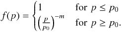 Above p0 the diffusion coefficient changes, where the power index m determines how quickly the acceleration time increases with increasing particle energy.
The form of the momentum diffusion coefficient (Eq. (37)) permits rewriting the reduced continuity Eq. (35) in dimensionless coordinates. The acceleration time τacc is the scale of a new dimensionless time coordinate x, and the new momentum coordinate  is normalized with the critical momentum p0 at which the behavior of the diffusion coefficient changes,
  (38)Written in these dimensionless coordinates the continuity Eq. (35) reads
  (39)and must be solved for 0 ≤ x ≤ T = zd/vadv/τacc, where T is the total available time in units of the acceleration time, previously estimated to be at most a few.
One immediately recognizes that the new equation depends on two parameters only. The parameter x represents the relation between the age of the system and its acceleration efficiency. Second, the power index m ∈ [0,1] of the momentum diffusion coefficient shapes particle spectra at  .
.
Note that the spatial and time coordinates are equivalent in our model. In the thin region of thickness zd behind the shock, where we expect strong turbulence, particle spectra will evolve as given in Eq. (39). As zd may be only a few per cent of a light-year, and the projection of spherical shells on the sky plane will distribute its emission over a large area, the spatial variation of the radio spectrum will probably not be resolvable by current radio observatories. Hence, it may suffice to calculate the average spectrum with the region of strong turbulence (colored light red in Fig. 1), for which we need to integrate the particle number density over time:  (40)Once particles have left the region of turbulence, their spectra will evolve little, because re-acceleration is by definition inefficient and energy losses are slow. For most of the volume between the contact discontinuity and the forward shock, shaded yellow in Fig. 1, we therefore expect the particle spectrum to be given by
  .
.
In the next section we will present solutions  for various x and m. Additionally, we demonstrate how different initial spectra impact the solution. In fact, modified shocks generate softer spectrum at low energies than predicted by DSA.
4. Results
4.1. Particle spectra
In the following we set N0 = 1 and initially N(p,t = 0) = N0p-2. In Fig. 2 we present the integrated particle number density, Nave, for different T but fixed power index m = 0.6 (cf. Eq. (37)). To be noted from the figure is the substantial flux enhancement near p0 even if the available time is only a fraction of the acceleration time. This demonstrates that stochastic reacceleration can be important in SNR, despite the relatively long acceleration time. The assumed turn-over in the momentum dependence of the diffusion coefficient at p/p0 = 1 causes the peak in Navep2 to be always close to p0.
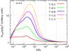 |
Fig. 2 Averaged electron number density, Nave, at different times T for fixed index, m = 0.6. |
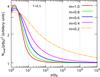 |
Fig. 3 Averaged electron number density, Nave, plotted for various power indices of the momentum diffusion coefficient, m, but fixed T = 0.5. |
The tail toward larger momenta is largely determined by the power index of the momentum diffusion coefficient, m. Figure 3 shows spectra for various m and fixed time T = 0.5. To be noted is that for small or moderate m the spectral bump near p0 has a high-energy tail that extends over more than 2 decades in momentum. To the outside observer that would appear as a softer spectrum at low momenta compared with that at very high momenta. The question arises to what degree the spectral modifications imposed by stochastic reacceleration depend on the initial spectrum produced at the shock. Recall that for Figs. 2 and 3 we assumed N(p,t = 0) = N0p-2, i.e. the test-particle solution for diffusive shock acceleration. Non-linear modification of the shock and the properties of the scattering turbulence upstream of the forward shock can soften or harden the initial spectrum. To test whether the effect of stochastic reacceleration downstream is largely independent of the initial spectrum, we plot in Fig. 4 the modification factor Nave/N(p,t = 0). For ease of exposition, the initial spectrum is assumed to follow a power law, N(t0) = N0p− s, where we vary the index s. The form of the momentum diffusion coefficient is as in Eq. (37) with fixed m. We observe that the choice of initial spectral index determines mainly the amplitude of the spectral bump, whereas its shape is weakly affected. There is degeneracy between the parameters m and T, visible, e.g., in the similarity of the spectral modification for T = 0.5 and s = 2.3 with that for T = 0.7 and s = 2.0. The initial conditions and the details of diffusive acceleration at the shock are largely irrelevant for the spectral characteristics provided by stochastic reacceleration in SNR.
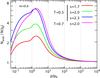 |
Fig. 4 Averaged electron number density, Nave, normalized by the initial distribution, N(t0) = N0p− s, plotted for different initial indices, s. |
4.2. Radio synchrotron emission
In strongly turbulent magnetic field with δB ≈ B0 the standard synchrotron emissivity is not applicable. In Appendix B we have derived an analytical approximation to the synchrotron emissivity for a turbulent field with Gaussian distribution of amplitudes (cf. Eq. (B.10)), that we shall use to calculate the radio spectral index. The main difference to the standard formula is a slower cut off ∝exp( − ν2/3).
Having established that the choice of initial particle spectrum plays a minor role and can be compensated with adjustments in the dimensionless time, we calculate radio spectra only for N(p,t = 0) = N0p-2, i.e. the radio spectral index at high frequencies is α = −0.5. As we use a dimensionless momentum coordinate, the synchrotron frequency is also dimensionless and normalized to the synchrotron frequency νx of electrons of momentum p0 in a magnetic field of amplitude Brms,  (41)The radio spectral index of the inner region, shaded yellow in Fig. 1, must be calculated with
  and is shown in Fig. 5. Note that it is at the same time the radio spectrum at the inner edge of the region of reacceleration, and so it reflects the final state of the electron spectrum after experiencing momentum diffusion for a time x = T = zd/vadv/τacc.
 |
Fig. 5 Radio spectral index of the far downstream region of an SNR, plotted for different times T and 2 choices of m. |
In Fig. 6 we present the radio spectral index, α, of the region in which we expect substantial momentum diffusion (shaded red in Fig. 1), i.e. computed using the average electron spectrum Nave. For ease of comparison, we chose the same time period, T, or thickness zd, and 2 choices of momentum dependence of the acceleration time at high energy.
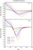 |
Fig. 6 Radio spectral index of the shell where reacceleration occurs, plotted for different times T and 2 choices of m. |
We have seen in Figs. 2–4 that a spectral bump results at a few p0. Consequently, the radio spectra below approximately 10 νx are hard, above 10 νx they are soft, and eventually they approach those provided by the forward shock, here taken as α = −0.5. The characteristics of the radio spectra are the following:
-
The spectral modification in the far downstream region (cf.Fig. 5) is slightly stronger than that in the shellwhere momentum diffusion operates, because all electrons fardownstream have sampled the full effect of reacceleration andhave since experienced little change in energy, whereas thespectrum in the immediate downstream reflects an average of thespectral modification as it builds up. The total radio spectrum willbe a mixture between the two.
-
Whenever the hardening at low frequencies below νx is significant, the spectral index changes rapidly with frequency, i.e. the spectral curvature is strong and should be detectable.
-
The softest spectra are observed at a few hundred to a thousand νx. For soft radio spectra from SNR it is therefore sufficient, if νx ≈ 10 MHz, corresponding to p0 ≈ 150 MeV /c for Brms ≈ 25 μG.
-
Less than one acceleration time is needed to soften the radio spectrum to α ≃ − 0.65. As the thickness of the acceleration region is zd = vadvTτacc, for a reacceleration time of a few years and an advection speed of 1000 km s-1 we find that a thickness of zd ≈ 3 × 10⁻³ pc is sufficient which in most cases is not resolvable.
-
If the increase of the reacceleration time scale with momentum is slow, i.e. m is small, soft radio spectra with very little curvature can be maintained over 3 decades in frequency. In contrast, for m = 0.6 spectral curvature is much stronger and should be detectable, in particular from the far downstream region.
5. Summary and conclusions
We have investigated the role of stochastic reacceleration in SNR with a view to probe whether or not it can account for the wide range of radio spectral indices observed among the more than 200 galactic SNR (Green 2009). Turbulence that can change a particle’s energy should be commonplace near the forward shocks of SNR. Cosmic-ray-driven instabilities operate in the upstream region. Other types of turbulence are excited at the shock itself. Whatever its nature, the turbulence will be advected to the downstream region where it has time to scatter energetic charged particles in pitch angle and momentum, until it is damped away. Reacceleration is therefore expected to be efficient, if anywhere, mostly in a potentially thin region behind the forward shock.
We calculated the momentum-diffusion coefficient for 3 types of turbulence, among which only transit-time damping of fast-mode waves operates on time scales of one or a few years. Incidentally, the energetic particles may be the dominant agent of damping for certain directions of wave propagation and thus harvest much of the turbulent energy. The acceleration time for transit-time damping of fast modes is found independent of energy, but expected to increase at higher energies on account of various inefficiencies.
In the case of small-scale non-resonant modes and the large-scale MHD turbulence arising from shock rippling, our estimates of the reacceleration rate are relatively simple. We feel that a more thorough treatment is not warranted on account of the long acceleration time that we derive. Transit-time damping of fast-mode waves is a much more promising process, for which we solve a resonance integral over the wave power spectrum. The main uncertainty here lies in the amplitude and spectral distribution of the waves, for which we here use generic arguments and cascading rates determined on the basis of detailed MHD simulations. While the wave power spectrum in a particular SNR will depend on the forward-shock speed and the properties of the upstream medium in that object, further work is needed to better understand the driving of fast-mode turbulence at astrophysical shocks with efficient particle acceleration.
Low-energy cosmic rays have a small mean free path, and so they are efficiently tied to the background plasma. Effectively, they advect on a characteristic in time t and the spatial coordinate z which describes the downstream distance to the forward shock. If reacceleration occurs only in a thin layer behind the shock, the cosmic-ray transport equation can be reduced to an initial-value problem, describing how the cosmic-ray spectrum is continuously deformed as the particles advect through the layer. Further inside, the particle spectrum is expected to change little and remain that calculated for the inner edge of the turbulence layer.
We numerically solved the reduced transport equation and found that cosmic-ray spectra develop a bump whose shape is largely independent of the initial spectrum assumed at the forward shock. To be noted is that the spectral bump can have an amplitude of a few hundred per cent, even if crossing the layer of efficient reacceleration takes less than one acceleration time. The shape of the high-energy tail of the bump depends on how quickly the acceleration time increases at high energies.
We calculated the synchrotron emissivity of electrons in a turbulent magnetic field with Gaussian distribution of amplitudes. Using that emissivity we determined the radio spectral index separately for the thin shell, where reacceleration occurs, and for the remaining interior of the SNR. The flux ratio between the two depends on the evolutionary history of the SNR and the supernova type, and so calculating total emission spectra can be done only once an object and its age are specified. Here, we only discuss the spectral index of radio emission from the two regions.
At low frequencies, where we observe particles subjected to reacceleration with energy-independent acceleration time, the radio synchrotron spectra tend to be hard with substantial curvature that should be evident in spectra covering 2 decades in frequency or more. Our results suggest that confusion with thermal or plerionic emission may be the culprit in cases of spectral indices close to α ≈ 0 extending over a large part of the radio band.
At higher frequencies, where we expect to see electrons that experienced momentum diffusion with an acceleration time increasing with particle energy, the radio synchrotron spectra are soft with indices α between −0.6 and −0.7 with little curvature for a slow increase of the diffusion coefficient with energy. About one acceleration time is sufficient to soften the radio spectrum by Δα ≃ − 0.15. The interiors of the remnants produce slightly softer radio spectra than does the shell where reacceleration occurs. Thus a modest reacceleration of electrons downstream of the forward shocks can explain the soft spectra observed from many galactic SNR.
Acknowledgments
We acknowledge support by the Helmholtz Alliance for Astroparticle Physics HAP funded by the Initiative and Networking Fund of the Helmholtz Association.
References
- Bell, A. R. 1978, MNRAS, 182, 147 [NASA ADS] [CrossRef] [Google Scholar]
- Bell, A. R. 2004, MNRAS, 353, 550 [Google Scholar]
- Blandford, R., & Eichler, D. 1987, Phys. Rep., 154, 1 [Google Scholar]
- Caprioli, D., Blasi, P., Amato, E., & Vietri, M. 2008, ApJ, 679, L139 [NASA ADS] [CrossRef] [Google Scholar]
- Cho, J., & Lazarian, A. 2002, Phys. Rev. Lett., 88, 245001 [Google Scholar]
- Crusius, A., & Schlickeiser, R. 1986, A&A, 164, L16 [NASA ADS] [Google Scholar]
- Drury, L. 1983, Space Sci. Rev., 36, 57 [NASA ADS] [CrossRef] [Google Scholar]
- Fatuzzo, M., & Melia, F. 2014, ApJ, 784, 131 [NASA ADS] [CrossRef] [Google Scholar]
- Fraschetti, F. 2013, ApJ, 770, 84 [NASA ADS] [CrossRef] [Google Scholar]
- Ghavamian, P., Laming, J. M., & Rakowski, C. E. 2007, ApJ, 654, L69 [NASA ADS] [CrossRef] [Google Scholar]
- Giacalone, J., & Jokipii, J. R. 2007, ApJ, 663, L41 [NASA ADS] [CrossRef] [Google Scholar]
- Green, D. A. 2009, Bull. Astron. Soc. India, 37, 45 [Google Scholar]
- Guo, F., Li, S., Li, H., et al. 2012, ApJ, 747, 98 [NASA ADS] [CrossRef] [Google Scholar]
- Inoue, T., Inutsuka, S.-i., & Koyama, H. 2006, ApJ, 652, 1331 [NASA ADS] [CrossRef] [Google Scholar]
- Inoue, T., Asano, K., & Ioka, K. 2011, ApJ, 734, 77 [NASA ADS] [CrossRef] [Google Scholar]
- Inoue, T., Yamazaki, R., Inutsuka, S.-i., & Fukui, Y. 2012, ApJ, 744, 71 [NASA ADS] [CrossRef] [Google Scholar]
- Kardashev, N. S. 1962, Sov. Astron., 6, 317 [NASA ADS] [Google Scholar]
- Koyama, K., Petre, R., Gotthelf, E. V., et al. 1995, Nature, 378, 255 [NASA ADS] [CrossRef] [Google Scholar]
- Lépine, S., & Moffat, A. F. J. 1999, ApJ, 514, 909 [NASA ADS] [CrossRef] [Google Scholar]
- Lépine, S., & Moffat, A. F. J. 2008, AJ, 136, 548 [NASA ADS] [CrossRef] [Google Scholar]
- Liu, S., Fan, Z.-H., Fryer, C. L., Wang, J.-M., & Li, H. 2008, ApJ, 683, L163 [NASA ADS] [CrossRef] [Google Scholar]
- Lucy, L. B., & White, R. L. 1980, ApJ, 241, 300 [NASA ADS] [CrossRef] [Google Scholar]
- Luo, Q., & Melrose, D. 2009, MNRAS, 397, 1402 [NASA ADS] [CrossRef] [Google Scholar]
- Lynn, J. W., Quataert, E., Chandran, B. D. G., & Parrish, I. J. 2013, ApJ, 777, 128 [NASA ADS] [CrossRef] [Google Scholar]
- Lynn, J. W., Quataert, E., Chandran, B. D. G., & Parrish, I. J. 2014, ApJ, 791, 71 [NASA ADS] [CrossRef] [Google Scholar]
- Malovichko, P., Voitenko, Y., & De Keyser, J. 2014, ApJ, 780, 175 [NASA ADS] [CrossRef] [Google Scholar]
- Mizuno, Y., Pohl, M., Niemiec, J., et al. 2011, ApJ, 726, 62 [NASA ADS] [CrossRef] [Google Scholar]
- Mizuno, Y., Pohl, M., Niemiec, J., et al. 2014, MNRAS, 439, 3490 [NASA ADS] [CrossRef] [Google Scholar]
- Niemiec, J., Pohl, M., Stroman, T., & Nishikawa, K.-I. 2008, ApJ, 684, 1174 [NASA ADS] [CrossRef] [Google Scholar]
- Oskinova, L. M., Hamann, W.-R., & Feldmeier, A. 2007, A&A, 476, 1331 [NASA ADS] [CrossRef] [EDP Sciences] [Google Scholar]
- Pelletier, G., Lemoine, M., & Marcowith, A. 2006, A&A, 453, 181 [NASA ADS] [CrossRef] [EDP Sciences] [Google Scholar]
- Petrosian, V. 2012, Space Sci. Rev., 173, 535 [NASA ADS] [CrossRef] [Google Scholar]
- Pohl, M. 1996, A&A, 307, L57 [NASA ADS] [Google Scholar]
- Pohl, M., Yan, H., & Lazarian, A. 2005, ApJ, 626, L101 [NASA ADS] [CrossRef] [Google Scholar]
- Prinja, R. K., & Massa, D. L. 2010, A&A, 521, L55 [Google Scholar]
- Ptuskin, V. S., & Zirakashvili, V. N. 2003, A&A, 403, 1 [NASA ADS] [CrossRef] [EDP Sciences] [Google Scholar]
- Quataert, E. 1998, ApJ, 500, 978 [NASA ADS] [CrossRef] [Google Scholar]
- Reville, B., Kirk, J. G., Duffy, P., & O’Sullivan, S. 2007, A&A, 475, 435 [NASA ADS] [CrossRef] [EDP Sciences] [Google Scholar]
- Reynolds, S. P. 2008, ARA&A, 46, 89 [Google Scholar]
- Runacres, M. C., & Owocki, S. P. 2002, A&A, 381, 1015 [NASA ADS] [CrossRef] [EDP Sciences] [Google Scholar]
- Schlickeiser, R. 2002, Cosmic Ray Astrophysics (Berlin: Springer) [Google Scholar]
- Shalchi, A. 2012, Phys. Plasmas, 19, 102901 [NASA ADS] [CrossRef] [Google Scholar]
- Shalchi, A., Koda, T. Å., Tautz, R. C., & Schlickeiser, R. 2009, A&A, 507, 589 [NASA ADS] [CrossRef] [EDP Sciences] [Google Scholar]
- Stroman, T., Pohl, M., & Niemiec, J. 2009, ApJ, 706, 38 [NASA ADS] [CrossRef] [Google Scholar]
- Vainio, R., & Schlickeiser, R. 1999, A&A, 343, 303 [NASA ADS] [Google Scholar]
- van Adelsberg, M., Heng, K., McCray, R., & Raymond, J. C. 2008, ApJ, 689, 1089 [CrossRef] [Google Scholar]
- Winske, D., & Leroy, M. M. 1984, J. Geophys. Res., 89, 2673 [NASA ADS] [CrossRef] [Google Scholar]
- Wong, R. 1989, Asymptotic Approximations of Integrals (Boston: Academic Press) [Google Scholar]
- Yan, H., & Lazarian, A. 2008, ApJ, 673, 942 [NASA ADS] [CrossRef] [Google Scholar]
- Zirakashvili, V. N., & Aharonian, F. A. 2010, ApJ, 708, 965 [NASA ADS] [CrossRef] [Google Scholar]
- Zirakashvili, V. N., Ptuskin, V. S., & Völk, H. J. 2008, ApJ, 678, 255 [NASA ADS] [CrossRef] [Google Scholar]
Appendix A: Solving the resonance integral for fast-mode waves
Appendix A.1: Parallel-propagating waves
For nearly parallel-propagating waves with μk = cosθk ≃ ± 1 we find for the angle-dependent wavelength, λc, at which the wave spectrum cuts off  (A.1)Note that there will be other damping mechanisms that will remove wave energy at some scale λmin, which we can treat as an upper limit to μk in the formula above.
If | μk | ≃ 1, then resonance is achieved at μ ≃ 0, and the term cs/ (μkc) in the argument of the exponential in Eq. (7) can be ignored. A change of integration variable  (A.2)turns Eq. (7) into
 ![\appendix \setcounter{section}{1} \begin{eqnarray} D_{\rm p}&\simeq&\frac{\sqrt{\pi}\,p^2\,c\,U_\mathrm{fm}}{8\,\epsilon\,B_0^2\,\beta\,\sqrt{\lambda_\mathrm{max}}}\, \int {\rm d}\mu_k\ \frac{\vert \mu_k\vert}{\sqrt{\lambda_{\rm c}}}\,\nonumber \\ &&\times \int_{-\infty}^\infty {\rm d}x\ \left(1+x^2\right)^{-3}\,\exp\left[-\frac{x^2}{\epsilon^2}\right]\cdot \label{eq:a2} \end{eqnarray}](/articles/aa/full_html/2015/02/aa25027-14/aa25027-14-eq185.png) (A.3)The second integral in x yields approximately ϵ for ϵ ≃ 0.5 − − 1. To compute the first integral we insert λc according to Eq. (A.1) and recall that there must be a limit λmin to the turbulence spectrum, thus finding
(A.3)The second integral in x yields approximately ϵ for ϵ ≃ 0.5 − − 1. To compute the first integral we insert λc according to Eq. (A.1) and recall that there must be a limit λmin to the turbulence spectrum, thus finding  (A.4)
(A.4)
Appendix A.2: Perpendicular-propagating waves
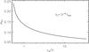 |
Fig. A.1 The critical wave direction, μk,c, as function of the velocity amplitude at the driving scale, V, below which λc = 10-6λmax. |
For nearly perpendicular-propagating modes with | μk | ≤ 0.39 damping by electrons dominates, and the cut off is found at  (A.5)Equation (A.5) suggests that the cut-off wavelength of cascading very rapidly falls off with decreasing μk. Figure A.1 displays the critical wave-angle cosine, μk,c, at which λc = 10-6λmax is reached for all | μk | ≤ μk,c. To be noted is that μk,c ≃ 0.1 for a wide range of velocity amplitudes, V, at the driving scale, λmax. For simplicity, we may therefore assume that λc = λmin = const. for all | μk | ≤ μk,c.
Then Eq. (7) can be written as ![\appendix \setcounter{section}{1} \begin{eqnarray} D_{\rm p}&\simeq&\frac{\sqrt{\pi}\,p^2\,c\,U_\mathrm{fm}}{8\,\epsilon\,B_0^2\,\beta\,\sqrt{\lambda_\mathrm{max}\,\lambda_\mathrm{min}}}\, \int {\rm d} \mu\ \left(1-\mu^2\right)^{3/2}\nonumber \\ &&\times \int_{-\mu_{k,{\rm c}}}^{\mu_{k,{\rm c}}} {\rm d} \mu_k\ \vert \mu_k\vert\, \exp\left[-\frac{(\mu-\frac{c_{\rm s}}{c\,\mu_k})^2}{\epsilon^2\,(1-\mu^2)}\right]\cdot \label{eq:a4} \end{eqnarray}](/articles/aa/full_html/2015/02/aa25027-14/aa25027-14-eq198.png) (A.6)Changing the variable of integration from μk to y = cs/ (cμk) simplifies this expression to
(A.6)Changing the variable of integration from μk to y = cs/ (cμk) simplifies this expression to ![\appendix \setcounter{section}{1} \begin{eqnarray} D_{\rm p}&\simeq &\frac{\sqrt{\pi}\,p^2\,c\,U_\mathrm{fm}}{4\,\epsilon\,B_0^2\,\beta\,\sqrt{\lambda_\mathrm{max}\,\lambda_\mathrm{min}}}\,\frac{c_{\rm s}^2}{c^2}\, \int {\rm d}\mu\ \left(1-\mu^2\right)^{3/2}\nonumber \\ &&\times \int_{\frac{c_{\rm s}}{c\,\mu_{k,{\rm c}}}}^\infty {\rm d}y\ \frac{1}{y^3}\,\exp\left[-\frac{(y-\mu)^2}{\epsilon^2\,(1-\mu^2)}\right]\cdot \label{eq:a5} \end{eqnarray}](/articles/aa/full_html/2015/02/aa25027-14/aa25027-14-eq200.png) (A.7)To be noted is that the lower limit of y-integration will be of the order 0.1 for SNRs. Given the form of the integrand in the second integral, small y will dominate the integral. Swapping the order of integration, approximating y ≪ 1 in the argument of the Gaussian, and reusing the variable transformation in Eq. (A.2), we find with reasonable accuracy
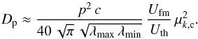
(A.7)To be noted is that the lower limit of y-integration will be of the order 0.1 for SNRs. Given the form of the integrand in the second integral, small y will dominate the integral. Swapping the order of integration, approximating y ≪ 1 in the argument of the Gaussian, and reusing the variable transformation in Eq. (A.2), we find with reasonable accuracy ![\appendix \setcounter{section}{1} \begin{eqnarray} D_{\rm p}&\approx &\frac{\sqrt{\pi}\,p^2\,c\,U_\mathrm{fm}}{4\,\epsilon\,B_0^2\,\beta\,\sqrt{\lambda_\mathrm{max}\,\lambda_\mathrm{min}}}\,\frac{c_{\rm s}^2}{c^2}\,\int_{\frac{c_{\rm s}}{c\,\mu_{k,{\rm c}}}}^\infty {\rm d}y\ \frac{1}{y^3}\, \nonumber \\ &&\times \int_{-\infty}^\infty {\rm d}x\ \frac{1}{\left(1+x^2\right)^{3}}\, \exp\left[-\frac{x^2}{\epsilon^2}\right]\cdot \label{eq:a6} \end{eqnarray}](/articles/aa/full_html/2015/02/aa25027-14/aa25027-14-eq203.png) (A.8)Both integrals can be easily solved separately to yield the final expression for the momentum diffusion coefficient. We already noted in Appendix A.1 that the second integral is approximately ϵ.
(A.8)Both integrals can be easily solved separately to yield the final expression for the momentum diffusion coefficient. We already noted in Appendix A.1 that the second integral is approximately ϵ. 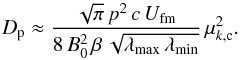 (A.9)which may be more conveniently written using the thermal energy density in the downstream plasma,
  ,
,  (A.10)
Appendix B: Synchrotron emissivity for turbulent magnetic field
For isotropic magnetic turbulence we may start with the angle-averaged spectral power per electron in a magnetic field of constant amplitude, which is well approximated with (Crusius & Schlickeiser 1986) 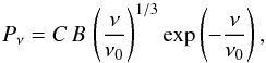 (B.1)where
  (B.2)We observe an individual electron radiating for only the Larmor period of a non-relativistic electron, which is considerably shorter than the period of the MHD waves that comprise the magnetic turbulence in SNRs. The instantaneous contribution to the synchrotron emissivity of an individual electron is therefore well described by a constant local magnetic acceleration, followed by averaging over all possible local magnetic-field strengths.
We suppose the magnetic-field amplitude follows a Gaussian probability distribution,  (B.3)The effective spectral power therefore is
 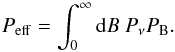 (B.4)Denoting x = B/Brms and νc = ν0(Brms) we find
![\appendix \setcounter{section}{2} \begin{eqnarray} P_\mathrm{eff} &=& \sqrt{\frac{2}{\pi}}\,C\,B_\mathrm{rms}\, \left(\frac{\nu}{\nu_{\rm c}}\right)^{1/3} \nonumber \\[2mm] &&\times \int_{0}^\infty {\rm d}x\ x^{2/3}\, \exp\left(-\frac{x^2}{2}-\frac{\nu}{\nu_{\rm c}\, x}\right)\cdot \label{eq:a13} \end{eqnarray}](/articles/aa/full_html/2015/02/aa25027-14/aa25027-14-eq213.png) (B.5)For ν ≪ νc the last exponential is irrelevant and the integral yields 1. The low-frequency spectral power therefore is
(B.5)For ν ≪ νc the last exponential is irrelevant and the integral yields 1. The low-frequency spectral power therefore is 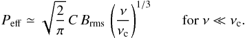 (B.6)For high frequencies, ν ≫ νc, we transform to y = x5/3, implying dy = (5/3) x2/3 dx. Then
![\appendix \setcounter{section}{2} \begin{eqnarray} P_\mathrm{eff} &= &\frac{6\,C\,B_\mathrm{rms}}{5\,\sqrt{2\pi}}\, \left(\frac{\nu}{\nu_{\rm c}}\right)^{1/3} \nonumber \\[2mm] &&\times \int_{0}^\infty {\rm d}y \ \exp\left(-\frac{y^{6/5}}{2}-\frac{\nu}{\nu_{\rm c}\, y^{3/5}}\right)\cdot \label{eq:a14} \end{eqnarray}](/articles/aa/full_html/2015/02/aa25027-14/aa25027-14-eq219.png) (B.7)We use the method of steepest ascent to solve the integral (e.g. Wong 1989). The negative argument of the exponential, exp[− F(y)], is Taylor-expanded around its minimum at y0 = (ν/νc)5/9, giving
(B.7)We use the method of steepest ascent to solve the integral (e.g. Wong 1989). The negative argument of the exponential, exp[− F(y)], is Taylor-expanded around its minimum at y0 = (ν/νc)5/9, giving  (B.8)The integral in Eq. (B.7) then reduces to a Gaussian and yields
 ![\appendix \setcounter{section}{2} \begin{eqnarray} P_\mathrm{eff} &\simeq&\frac{C\,B_\mathrm{rms}}{\sqrt{3}}\, \left(\frac{\nu}{\nu_{\rm c}}\right)^{5/9}\, \exp\left(-\frac{3}{2}\,\left(\frac{\nu}{\nu_{\rm c}}\right)^{2/3}\right)\nonumber \\[2mm] &&\times \left(1+\mathrm{erf}\left[\sqrt{\frac{27}{50}}\, \left(\frac{\nu}{\nu_{\rm c}}\right)^{1/3}\right]\right)\cdot \label{eq:a16} \end{eqnarray}](/articles/aa/full_html/2015/02/aa25027-14/aa25027-14-eq223.png) (B.9)This is the high-frequency solution to the integral in Eq. (B.5) which we need to combine with the low-frequency solution given in Eq. (B.6). Noting that the argument of the error function is slowly varying, we can replace the error function with a constant that is appropriate for frequencies slightly above ν0. We know that the normalization of the spectral power has to match that for a homogeneous magnetic field with B = Brms, because the energy loss rate is quadratic in B. Using an algebraic transition that is accurate in the normalization to within 1% and matches the asymptotic behavior, we finally obtain
(B.9)This is the high-frequency solution to the integral in Eq. (B.5) which we need to combine with the low-frequency solution given in Eq. (B.6). Noting that the argument of the error function is slowly varying, we can replace the error function with a constant that is appropriate for frequencies slightly above ν0. We know that the normalization of the spectral power has to match that for a homogeneous magnetic field with B = Brms, because the energy loss rate is quadratic in B. Using an algebraic transition that is accurate in the normalization to within 1% and matches the asymptotic behavior, we finally obtain ![\appendix \setcounter{section}{2} \begin{eqnarray} P_\mathrm{eff} &\simeq &C\,B_\mathrm{rms}\,\sqrt{\frac{2}{\pi}}\, \left(\frac{\nu}{\nu_{\rm c}}\right)^{1/3} \, \exp\left(-\frac{3}{2}\,\left(\frac{\nu}{\nu_{\rm c}}\right)^{2/3}\right)\nonumber \\[2mm] &&\times \left(1+1.65\,\left(\frac{\nu}{\nu_{\rm c}}\right)^{0.42}\right)^{0.53}\cdot \label{eq:a17} \end{eqnarray}](/articles/aa/full_html/2015/02/aa25027-14/aa25027-14-eq227.png) (B.10)A comparison with the standard formula (Eq. (B.1)) is given in Fig. B.1. A corresponding formula for an exponential distribution of magnetic-field amplitudes can be found in Zirakashvili & Aharonian (2010).
(B.10)A comparison with the standard formula (Eq. (B.1)) is given in Fig. B.1. A corresponding formula for an exponential distribution of magnetic-field amplitudes can be found in Zirakashvili & Aharonian (2010).
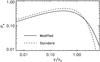 |
Fig. B.1 Comparison of the standard expression for the spectral synchrotron power of electrons with that derived here for turbulent magnetic field with Gaussian distribution. |
All Figures
|
Fig. 1 Schematic representation of the scenario. In a region of thickness zd behind the forward shock (FS) turbulence can re-accelerate electrons. |
| In the text | |
|
Fig. 2 Averaged electron number density, Nave, at different times T for fixed index, m = 0.6. |
| In the text | |
|
Fig. 3 Averaged electron number density, Nave, plotted for various power indices of the momentum diffusion coefficient, m, but fixed T = 0.5. |
| In the text | |
|
Fig. 4 Averaged electron number density, Nave, normalized by the initial distribution, N(t0) = N0p− s, plotted for different initial indices, s. |
| In the text | |
|
Fig. 5 Radio spectral index of the far downstream region of an SNR, plotted for different times T and 2 choices of m. |
| In the text | |
|
Fig. 6 Radio spectral index of the shell where reacceleration occurs, plotted for different times T and 2 choices of m. |
| In the text | |
|
Fig. A.1 The critical wave direction, μk,c, as function of the velocity amplitude at the driving scale, V, below which λc = 10-6λmax. |
| In the text | |
|
Fig. B.1 Comparison of the standard expression for the spectral synchrotron power of electrons with that derived here for turbulent magnetic field with Gaussian distribution. |
| In the text | |
Current usage metrics show cumulative count of Article Views (full-text article views including HTML views, PDF and ePub downloads, according to the available data) and Abstracts Views on Vision4Press platform.
Data correspond to usage on the plateform after 2015. The current usage metrics is available 48-96 hours after online publication and is updated daily on week days.
Initial download of the metrics may take a while.