| Issue |
A&A
Volume 574, February 2015
|
|
|---|---|---|
| Article Number | A76 | |
| Number of page(s) | 7 | |
| Section | Astronomical instrumentation | |
| DOI | https://doi.org/10.1051/0004-6361/201424882 | |
| Published online | 28 January 2015 | |
Tachoastrometry: astrometry with radial velocities
1
ESO, Karl-Schwarzschild-Strße 2, 85748
Garching bei München,
Germany
e-mail:
This email address is being protected from spambots. You need JavaScript enabled to view it.
2
Departamento de Física, Facultad de Ciencias Básicas, Universidad
Metropolitana de Ciencias de la Educación, Av. José Pedro Alessandri 774, 7760197 Ñuñoa,
Santiago,
Chile
3
The Millennium Institute of Astrophysics (MAS),
Cassilla 36- D Santiago, Chile
4
University of Milan, Department of Physics,
via Celoria 16, 20133
Milan,
Italy
5
ESO, Alcnso de
Córdova 3107, Vitacura, Cassilla 19001, Santiago, Chile
6
Departamento de Física, Universidade Federal do Rio Grande do
Norte, 59072-970,
Natal, RN
Brazil
Received: 29 August 2014
Accepted: 12 December 2014
Abstract
Context. Spectra of composite systems (e.g., spectroscopic binaries) contain spatial information that can be retrieved by measuring the radial velocities (i.e., Doppler shifts) of the components in four observations with the slit rotated by 90 degrees in the sky.
Aims. We aim at developing a framework to describe the method and to test its capabilities in a real case.
Methods. By using basic concepts of slit spectroscopy we show that the geometry of composite systems can be reliably retrieved by measuring only radial velocity differences taken with different slit angles. The spatial resolution is determined by the precision with which differential radial velocities can be measured.
Results. We use the UVES spectrograph at the VLT to observe the known spectroscopic binary star HD 188088 (HIP 97944), which has a maximum expected separation of 23 milli-arcseconds. We measure an astrometric signal in radial velocity of 276 m s-1 , which corresponds to a separation between the two components at the time of the observations of 18 ± 2 milli-arcseconds. The stars were aligned east-west. We describe a simple optical device to simultaneously record pairs of spectra rotated by 180 degrees, thus reducing systematic effects. We compute and provide the function expressing the shift of the centroid of a seeing-limited image in the presence of a narrow slit.
Conclusions. The proposed technique is simple to use and our test shows that it is amenable for deriving astrometry with milli-arcsecond accuracy or better, beyond the diffraction limit of the telescope. The technique can be further improved by using simple devices to simultaneously record the spectra with 180 degrees angles. This device together with an optimized data analysis will further reduce the measurement errors. With tachoastrometry, radial velocities and astrometric positions can be measured simultaneously for many double line system binaries in an easy way. The method is not limited to binary stars, but can be applied to any astrophysical configuration in which spectral lines are generated by separate (non-rotational symmetric) regions.
Key words: techniques: high angular resolution / techniques: radial velocities / techniques: spectroscopic / binaries: spectroscopic
© ESO, 2015
1. Introduction
The quest to obtain high angular resolution and astrometric information from ground-based telescopes is quite pressing, in particular after adaptive optics (AO) and optical interferometry have shown its tremendous potential for obtaining sharp images and precise astrometry. At the same time, prompted mostly by planet search and the study of stellar oscillations, radial velocity precision has dramatically improved as well (Anderson et al. 2008), reaching below the m s-1 (Mayor et al. 2003). The basic idea behind this work is that astrometry and radial velocity are in many instances intimately connected.
Three decades ago a method to determine the distance between two stars of a binary system using radial velocity measurements was suggested (Beckers 1984). In this paper we reconsider this idea, prove its feasibility, discuss its application to different astrophysical situations, and provide a simple optical concept to improve the accuracy of the method. In the last 15 years, several spectroscopic techniques have been developed to retrieve astrometric information. Following the seminal paper by Beckers (1983), Bailey (1998) developed spectroastrometry and applied it to the observation of young stars. Spectroastrometry is now used with success on other objects, from planetary nebulae (Blanco Cárdenas et al. 2014) to active galactic nuclei (Gnerucci et al. 2013). The technique proposed in this work is related to spectroastrometry, but it is at the same time substantially different because it ignores the spatial profile of the recorded spectra, and relies uniquely on measured Doppler velocities (which is why the name tachoastrometry is used).
With tachoastrometry the measurable angular separation depends only on its abilty to measure Doppler shift differences in the spectral lines of the observed objects. The achievable angular resolution depends only on the ratio between the precision of the Doppler measurement and the slit scale.
2. Concept
The fundamental concept is very simple. In a grating spectrograph, the image at the telescope focal plane (or the slit) is re-imaged and dispersed on the spectrograph detector. A source moving in the slit plane will move in the detector plane, by an amount given by1 (1)where \begin{lxirformule}$\Delta x_\mathrm{det}$\end{lxirformule} and Δxslit are the shift at the slit and at the detector, and Fcam and Fcol are the focal length of the camera and of the collimator, respectively.
By moving the object along the slit (i.e., perpendicular to dispersion), the spectrum is shifted along the spatial direction; by moving the object across the slit in the direction of the dispersion, a wavelength shift is thus produced in the observed spectrum, which will induce an observed Doppler shift. The amount of the shift is given by (1), but can be transformed in km s-1 by using the spectrograph linear dispersion (Δλ/ mm) and the wavelength:  (2)Using the standard
  , this brings to
  (3)This can also be expressed in arcseconds for any spectrograph by transforming Δxslit into α (arcsec). A simple, convenient way of expressing the shift is given by
  (4)where R is the spectrograph resolving power for 1 arcsec slit aperture and c is the speed of light in km s-1 . In a conventional spectrograph the resolving power changes with wavelength, and so will the scale conversion factor. In an echelle spectrograph, R is approximately constant with wavelength, and so is the conversion factor.
These are optical relationships. In real observations of a point-like, seeing-limited astronomical object, the shift of the image after the spectrograph slit is smaller than the shift of the object in the focal plane because the effects of a finite slit must be taken into account. Its computation is given in the Appendix. In all cases, artificial Doppler shifts induced by the slit centering error may be considerable and this is a well-known limitation to measuring precise radial velocities. A considerable effort has been devoted to eliminating this effect, either by scrambling the source light with fibers and other optical systems, as done, for instance in HARPS (Mayor et al. 2003), or by using a gas cell in the optical path as a direct reference source (Beckers 1977).
Calling RVm the measured radial velocity of a star (formally called measured Doppler shift; see Lindegren & Dravins 2003 for a definition of radial velocity, but hereafter we use radial velocity as a common term), this can be expressed as  (5)where RVspectro and RVslit are the shifts induced by spectrograph instabilities and by object centering errors, respectively.
The aim of this work is to show that in special circumstances, for instance in the presence of a binary star, instead of trying to eliminate the contribution of RVslit, this can be successfully used to retrieve the geometry of the system.
For a spectroscopic binary with double line system (SB2) the measured RV difference between the two components will not be determined only by the true RV difference between the stars, but will also contain a geometrical component produced by the distance between the two stars along the spectrograph dispersion axis. Because the two stars of the spectroscopic binary are observed simultaneously and along the same optical path, RVspectro is the same for both stars, so it will not contribute to their RV difference.
The principle is shown in Fig. 1, with two stars separated by a distance D in the sky, and a distance Dcosθ projected along the slit width, with θ being the projected angle between the line joining the two stars and the dispersion direction. In the example we assume that the two stars have true radial velocities RV1 and RV2 at the source.
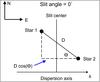 |
Fig. 1 Description of the geometry of the stars and spectrograph slit during the first observation: the observed difference in radial velocity between the stars depends on their true difference in RV and on their separation in the sky. |
With the first observation, we measure therefore a RV difference ΔV1 (see Fig. 1):  (6)A second measurement is acquired by rotating the slit by 180 degrees in a time sequence short enough that RV1 and RV2 can be considered constant; the geometry is given in Fig. 2. In this case, the difference in the observed RV of the stars is given by
  (7)therefore, with a simple difference we find
 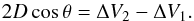 (8)By taking two additional exposures, rotating the slit orientation by 90 and 270 degrees and measuring ΔV3 and ΔV4, the full geometry of the system is solved:
 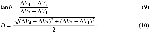 The astrometric information (separation and angle) is obtained by measuring differences in radial velocities; therefore, the sensitivity of the method is determined by the capability of measuring precise radial velocities. This is extremely attractive for cool stars, for instance, that have thousands of narrow spectral lines, for which a RV precision close to or better than 1 m s-1 can be obtained. Because we measure velocity differences in the same spectrum, and in spectra taken within a short time interval, most systematic effects are canceled out and there is no need for a long-term instrumental stability. To obtain a reference example, a radial velocity difference of 1 m s-1 on UVES at the VLT (Dekker et al. 2000), for which 1 arcsec is equal to 7.5 km s-1 , corresponds to an angular separation α = 1.33 × 10⁻⁴ arcsec (133 micro arcseconds), which is several times better than the VLT diffraction limit in the visible. If not limited by other factors, this method will therefore open interesting opportunities.
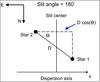 |
Fig. 2 As in Fig. 1, but now the slit has been rotated by 180 degrees. The measured difference in radial velocity between Figs. 1 and 2 will depend on the projected separation of the stars along the dispersion. |
3. Measurement uncertainties
3.1. Instrumental error budget
Relations 9 and 10 show that the astrometric precision depends on the error on how the RV difference can be measured (hereafter δDV) as  and
and  provided, of course, that distance and velocity are expressed in the same units. As predicted, the precision with which the radial velocity difference can be measured is directly related to the precision of the geometrical parameters. This error assumes that other source of uncertainties, such as the rotation angle of the slit, are negligible. This is the case for all modern instrument adaptors. Another source of instrumental uncertainty is the stability with time of the linear dispersion Δλ/mm. This can vary, for instance, because of variations in temperature or pressure. UVES is a very stable instrument, so linear dispersion variability is not an issue within the duration of one cycle and even for much longer timescales. In our tests we checked the spectrograph pressure and temperature stability during our observations; for less stable spectrographs, frequent wavelength calibrations should be taken. We note that it is possible to use calibrations taken with a small slit and use them for the wide slit observations because what matters is the stability of the linear dispersion, which does not depend on the slit width.
3.2. Seeing, slit losses
In all cases of astrophysical interest the two sources will appear blended because of the diffraction limit of the telescope and because of the seeing. Seeing will not directly affect the measurements because at these scales (much less than one arc-second) isoplanatism is guaranteed in all atmospheric conditions even at visible light; this implies that both stars images suffer exactly of the same wavefront deformations induced by seeing. The images of the stars will wander on the focal plane, but always in the same way for both objects, which is important for our case. This implies that the relative position between the two stars will not change, and therefore the difference in radial velocities induced by their geometric distance will not be affected by the seeing.
When a small slit is used, because the stars are not perfectly centered in the slit, their flux is cut asymmetrically by the slit jaws. The vignetting will introduce a systematic effect, as discussed in the introduction, that will affect the RV of both stars in a similar way. However, the two stars do not have exactly the same position. In the presence of a narrow slit, the distance measured after the slit is smaller than the real distance in the sky. This effect will be small in most circumstances, because the stars will not be very far apart, but still present and so a correction must be applied. The measured distance between the stars will be compressed with respect to the real distance in the sky by a quantity given by Eq. (A.1). Our tests include observations with narrow and wide slit and the results are in excellent agreement with what predicted by Eq. (A.1).
In order to safely cope with this problem we will use a large slit. This may induce large variations in the observed spectral profiles between the four observations if seeing variations between the exposures occur. With a large slit the spectrograph point spread function (PSF) is determined by the seeing. Large PSF variations may complicate the analysis and the measurement of the RV, because the observations separated by 180 degrees are not carried out simultaneously. In general, variation of the line profiles will lower the precision of the RV measurements. The appropriate measurement of the RV and a composite and variable instrumental line profile might introduce noise in the measurements. The problem of fitting a double function without knowing the exact PSF has been addressed in the literature, and, in order to derive accurate radial velocity measurements in composite spectra of binary stars, ad hoc methods have been developed. For instance Zucker et al. (2003) improve the performances of a simple cross-correlation analysis by optimizing the spectra of each component with a proper spectral match. We consider the optimization of the data analysis to be beyond the scope of the present work, but we believe that the method can be improved by simultaneously acquiring observations at different angles by constructing a simple optical device, and we present a possible design for such a device in Sect. 7.
3.3. Source variability
Tachoastrometry assumes that the sources have constant radial velocity during the observations. The validity of this assumption depends on the nature of the object observed and on the precision requested. The best test cases with which to investigate the validity of this hypothesis are solar-type stars. In these stars stellar oscillations, long-term magnetic cycles, and rotational modulation affect the radial velocity constancy with different timescales. All these effects must be taken into consideration when searching for low mass planetary companions, as in the case of αCen B, which was studied by Dumusque et al. (2012). Magnetic cycles, similar to the solar 11-year cycle, can induce radial velocity variations of several m s-1 (Dumusque et al. 2012), but these cycles are effective on long timescales of several years, which are generally of no interest for tachoastrometry. Instead, solar-type oscillations affect radial velocities with short timescales, at the level of a few m s-1 (Kjeldsen et al. 2005), with an amplitude that depends on the stellar effective temperature and gravity. Similarly, rotational modulation can produce radial velocity modulation at a level of up to several m s-1 depending on the chromospheric activity level of the stars (Dumusque et al. 2012; Paulson et al. 2004). For astrometric measurements that aim at the highest precision comparable to or below the m s-1, these effects must be taken into account. As far as stellar oscillations are concerned, many short observations can be acquired, or observations long enough (on the order of 15 min) to average out the oscillation signal. Rotational modulation should instead be modeled, as done in exoplanet searches. It is likely, however, that the presence of this variability will set the ultimate precision of tachoastrometry for binary stars to a few m s-1.
4. The test
We tested the method by observing the binary HD 188088 (HIP 97944) with the UVES spectrograph on the VLT (Dekker et al. 2000) with the standard red arm setup centered at 580 nm. The star was carefully selected because the most appopriate object has to fulfill a number of characteristics: the expected effect should be conveniently measurable, therefore the angular separation should vary between a few tenths and a few hundreds of arcseconds; the star should be a double line spectroscopic binary, to see both line systems; the stars should also be late-type and slow rotators, in order to obtain precise radial velocity measurements. After all the criteria were applied, we chose HD 188088 (HIP 97944), whose characteristics are summarized in Table 1. HD 188088 is a binary formed by two K3V stars (Torres et al. 2006), with similar masses and luminosities (~ 0.86 M⊙) with a period of 46.817 d and a high eccentric (0.69) orbit (Fekel & Beavers 1983).
Orbital elements of HD 188088.
The observations were carried out as technical tests on September 6, 2013. Two cycles were obtained: the first using a slit width of 1 arcsec; single integrations were short, thanks to the relative brightness of the sources. For the second cycle we used a wide (5 arcsec) slit width. By acquiring these two cycles we are able to the compare the results with the predictions of the effects expected by using a small slit. Each cycle is composed of seven observations, because observations at 0 degree orientation were repeated, even after a full 360 degree rotation. Each cycle took in total less than 13 min, each exposure being 40 or 60 s long, providing a signal-to-noise ratio (S/N) of at least 250 at 5750 Å for each spectrum. The seeing during the observations was good, and almost constant around 0.7 arcsec, and the values are reported, together with the other main observation parameters in Table 2. Some reduced spectra around the LI (~6708 Å) are presented in Fig. 3, where the duplicity of the spectra is evident, and the lines of the two stars are clearly separated.
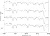 |
Fig. 3 Spectra HD 188088 for different slit angles. The lines of the two stars are clearly separated in the spectra. |
Ephemerides of the observations of HD 188088, time is UT on September 6, 2013.
5. Results
After data reduction, the radial velocity analysis was carried out by using a digital cross-correlation mask (Melo et al. 2001). We used two Gaussian functions to fit the double peaked cross-correlation function (CCF; Tonry & Davis 1979) and to measure the RVs of each star. Since the rotational velocity of both components is low (see Table 2), the Gaussian function is adequate to obtain a good representation of the CCF profiles, and we leave the Gaussian widths, intensities, and centers as free parameters. The results of the single measurements are given in Table 3 in which the widths of the Gaussian function σ resulting from the best fit are also reported. Figure 4 shows a typical CCF profile, where it can be noticed that the CCF has low level side lobes that alter the continuum, most likely produced by an imperfect match of the mask used with the stellar spectrum, or by a low level residual fringing. For future observations, it might be useful to observe a slowly rotating single star of similar spectral type to produce an empirical CCF profile, or to optimize the digital mask to the spectrum of the observed star. We have performed many tests by varying the CCF fit window over a large range. A small window allows very good fits of the CCF cores (and therefore a very small nominal error in the centers), but poses poor constraints on the wings, leading to unacceptable differences in the separations between the CCF peaks in the two cycles. Large windows are very sensitive to the continuum fluctuations, fail to satisfactorily reproduce the cores, and thus provide a large error. However, while the RV measurements can vary by several tens of m s-1 depending on the fitting window adopted, it is remarkable that the effects are systematic and the ΔVi − ΔVi − 1 measurements are extremely robust, within a few (± 5) m s-1 independent of the continuum window chosen. In Table 4 the measured velocity differences and results are summarized. In the following we use the results from a ± 50 km s-1 window.
Computed radial velocities RV for HD 188088.
Derived D and θ for HD 188088.
Cycle 1: the error estimated by the fit for each radial velocity is 19 m s-1 , constant for all observations, and the same for the two stars. The repeated observations at 0 and 360 degree show a good consistency in the radial velocity difference between the two stars. The average difference for this angle is of 13.376 km s-1 , with a maximum deviation from the average of 26 m s-1 . We use this average value for ΔV1 for 0 degrees for cycle 1.
We note that the 0−360 degree observations made at the end of both cycles are slightly smaller than the one made at the beginning. This is consistent with the fact that, according to the published ephemerides, at the time of the observations the phase was just above 0.5, and the radial velocities of the two stars are predicted to become closer with time.
We believe that the difference in the measured values is the most realistic error estimate for the velocity difference ΔV in the CCF. It is worth noticing that the last observation of the cycle was performed after a full 360 degree rotation of the slit. The results show that no major effects are produced by the full adapter rotation, because the last two exposures of the cycle agree at better than 10 m s-1. The difference between the 90 and 270 degree observations is negligible ΔV4 − ΔV3 = (0 m s-1), while the difference between 0 and 180 degrees, ΔV2 − ΔV1, is quite pronounced (185 m s-1), showing that at the time of the observations the two stars were almost perfectly E-W oriented.
Cycle 2: the estimated error on the single measurement is higher (32 m s-1) and the σ slightly larger. This is expected from the use of the large slit. The measurement at 0 and 360 degrees, are also consistent, with an average value of ΔV1 = 13.300 m s-1 and a maximum deviation from the average of 17 m s-1. Also in this case, the largest difference is between the 0 and 180 degree orientation, with ΔV2 − ΔV1 = 276 m s-1, while ΔV4 − ΔV3 = −4 m s-1 confirming the negligible separation of the two stars in the N-S direction.
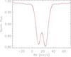 |
Fig. 4 Example of cross-correlation function (black line) and fit (red line) for our observations. |
Both cycles are very consistent. They show a pronounced ΔV2 − ΔV1 difference, while the ΔV4 − ΔV3 difference is negligible (0 and − 4 m s-1 respectively for cycle 1 and 2). This indicates that at the moment of the observations the two components of the binary were almost perfectly aligned E-W. The resulting distance is of 12 ± 2 milliarcseconds for cycle 1 and of 18 ± 2 milliarcsec for cycle 2, the error being determined by the error formula and a δDV of 26 m s-1 , as determined from the repeated observations at 0 and 360 degrees for both cycles. As predicted in Sect. 3.2, the cycle 1 observations provide a smaller separation, because they were acquired with a small slit.
We estimate the correction to be applied to the first cycle expected by the use of 1 arcsec slit. We used as input to Eq. (A.1) the observational values (seeing =0.7 arcsec, separation between the stars of 0.018 arcsec, as measured in the second cycle, slit width 1 arcsec). Equation (A.1) predicts for the first cycle an observed value of Δxobs = 11 milliarcsec, and we measured 12. A correction of 7 milliarcsec has to be added to the cycle 1 result. This brings the corrected cycle 1 distance to 19 milliarcsec, in excellent agreement with the wide slit cycle 2 results. The correction to be applied for the cycle 1 observations (seeing =0.7 arcsec, slit width =1 arcsec) is therefore not negligible and critically depends on the seeing value. For the UVES observations, we have two independent ways of measuring the seeing: from the height of the observed spectra, and from the values provided by the telescope at the beginning and at the end of the observations. They agree very well and, as seen from Table 2, the seeing varied by less than ± 5% during our observations. In order to evaluate the error associated with the correction applied, we use the simplified formula (12). By differentiating Eq. (12) the uncertainty for the correction is found: δ ⟨ x ⟩ / ⟨ x ⟩ = 2δσ/σ. This implies that the uncertainty associated with the correction applied to cycle 1 is less than 10% of the correction, or 0.7 milliarcsec. This shows a robust result but, as we anticipated, observing with a slit wide enough to avoid slit corrections seems the safest choice. It is nevertheless very encouraging that the two cycles give results in excellent agreement, providing at the same time a nice test of the whole procedure.
The results are very consistent and provide a robust distance of 18 ± 2 milli-arcsec between the stars and a separation angle of − 0.4 ± 5 degrees. In this first application a precision of a few milli-arcseconds is obtained, which can be considered very satisfactory for a first test and shows the potentiality of the method.
6. Discussion
Applying tachoastrometry to double line spectroscopic binaries enables us to simultaneously obtain the radial velocity curve and the geometry of the systems, providing the separation and the angle between the stars. In this way it will be possible to determine full orbits for SB2 stars, without the need of interferometric observations. SB2 full orbital solutions provide accurate masses and distances (see, e.g., Pourbaix 1998). With tachostrometry distances and masses of SB2 up to several hundred parsecs could be determined, providing access to special classes of objects, such as young stars and nearby clusters and associations. The concept of SB2 in this context should be considered in a wide sense because it will be also possible to separate stars in distant regions that appear unresolved because of the limited spatial resolution of the telescope, and it is not required that the stars belong to a physical binary system.
It is worth mentioning that, to the best of our knowledge, the geometrical component has been so far ignored when solving the radial velocity curves of SB2. The geometrical effect can introduce systematic effects in the K1 and K2 estimates, or can simply add noise to the measurements, depending on the slit orientation used. The effect is clearly small (~300 m s-1 for the star we observed), but might not be negligible when very accurate measurements are needed. It is comparable to or larger than the measurement errors of the radial velocities.
Even if we used SB2 stars to introduce the concept of tachoastrometry, in principle this technique can be applied to all systems showing composite spectra. In all astrophysical situations where resolved spectral lines are produced in physically distinct regions, tachoastrometry can be applied. Interesting examples could be stars surrounded by asymmetric disks, binaries with low mass companions, novae, supernovae, or quasars. In all these cases, the emission and absorption line systems (or continuum) are well separated and may originate in physically distinct places. It might not be trivial to use the technique, but there is no reason why it should not apply. Some of the over mentioned sources have rather broad lines, up to many km s-1 , so the use of Doppler shift measurements at the few m s-1 precision could be questioned. Indeed, obtaining accurate velocity measurements for broad lines is impossible, but it is important to note that in tachoastrometry the angular resolution is given by the ratio between the measured velocity shift and the resolving power. So, the resolving power of the spectrograph should match the line width of the observed objects. In the case of spectral lines thousands of km s-1 wide, one can aim to measure shifts with only a few km s-1 precision. In this case a low resolution spectrograph will be used. What actually determines the angular resolution is only the ratio between the Doppler velocity precision and the spectrograph scale at the slit (expressed in km s-1). So in the case of broad lines, a spectrograph with a resolving power of 300 for 1 arcsec slit will still produce 1 milli-arcsec resolution if a velocity precision of 1 km s-1 is obtained.
Even single stars could be sources of observations, if we consider that different lines can be formed in spatially distinct structures. The best known are probably the core of the deep absorption lines, such as Ca II H and K, which are formed in the stellar chromosphere. These lines are enhanced in active regions, and vary with the stellar rotation period because of the inhomogeneities on the stellar surface. Applying tachoastrometry differentially to chromospheric and photospheric lines would provide the position of the active region with respect to the stellar center. Similarly, lines that are very temperature sensitive strongly react to the presence of cool spots and modulate their intensities thanks to the appearance and rotation of strong spots. Doppler imaging has been developed over the years to interpret these variations and to produce stellar maps. The proposed technique can in principle measure the angle of the rotating inhomogeneities on a stellar disk, even for stars that do not rotate at a fast rate.
We should finally discuss tachoastrometry with respect to spectroastrometry. They originate from the same work (Beckers 1983) although they are substantially different in their applications. Tachoastrometry does not bring more information than spectroastrometry, but it is extremely simple to use. It has a more restricted range of applications; for instance, it cannot be applied to systems only with continuum because it is sensitive to spectral lines. In principle, both techniques are limited by the S/N and only application to real objects and experience will reveal their real sensitivity limits. We finally note that tachoastrometry does not depend on the telescope size or on site quality; it allows small telescopes to reach a very good spatial resolution in sites that are not optimal and without the support of AO
7. A simple device to simultaneously record opposite angles
It is possible to design a simple device that allows the simultaneous acquisition of two spectra taken with opposite (180 degrees) slit orientation angles. Such a device would improve the quality of the observations and optimize the data reduction, because the two spectra would be acquired simultaneously and with exactly the same instrumental configuration. The device should be able to rotate the slit by 180 degrees, keeping the two images co-focal. The simplest way to rotate an image is to use an odd number of reflections. Figure 5 shows a possible device, adapted for the UVES spectrograph. The device is located before the spectrograph slit, in front of the slit plane and the non-dispersed light, coming from the telescope on the left side, is first divided into two halves by a beamsplitter. Half of them pass through a system of five reflections while the others are not deviated, but pass through a glass layer that compensates for the shorter optical path, so that the two paths have the same focal distance.
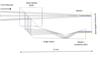 |
Fig. 5 Optical design of a simple device to simultaneously record spectra with 180 degree orientation. The design is optimized for the UVES spectrograph. The rays with different colors do not represent different wavelengths, rather the geometrical position of the extremes, to show visually how the green ray, which is located at the upper limit at the entrance, and the blue ray, which is located at the lower extreme, maintain the geometry in slit 1 while they are geometrically rotated in slit 2, after an odd number of reflections. |
We neglect in this equation important effects, such as grating anamorphism. In a real system Δx changes with wavelength.
Acknowledgments
L.P. thanks J. Beckers for enlightening discussions while observing many years ago at the ESO 3.6 m telescope. He also acknowledges the Visiting Researcher program of the CNPq Brazilian Agency, at the Fed. Univ. of Rio Grande do Norte, Brazil. Support for C.C. is provided by the Ministry for the Economy, Development, and Tourism’s Programa Iniciativa Científica Milenio through grant IC 120009, awarded to the Millennium Institute of Astrophysics (MAS).
References
- Anderson, J., Sarajedini, A., Bedin, L. R., et al. 2008, AJ, 135, 2055 [NASA ADS] [CrossRef] [Google Scholar]
- Bailey, J. A. 1998, in Optical Astronomical Instrumentation, ed. S. D’Odorico, SPIE Conf. Ser., 3355, 932 [Google Scholar]
- Beckers, J. M. 1977, ApJ, 213, 900 [NASA ADS] [CrossRef] [Google Scholar]
- Beckers, J. M. 1983, Lowell Observatory Bulletin, 9, 165 [NASA ADS] [Google Scholar]
- Beckers, J. M. 1984, BAAS, 16, 498 [NASA ADS] [Google Scholar]
- Blanco Cárdenas, M. W., Käufl, H. U., Guerrero, M. A., Miranda, L. F., & Seifahrt, A. 2014, A&A, 566, A133 [NASA ADS] [CrossRef] [EDP Sciences] [Google Scholar]
- Dekker, H., D’Odorico, S., Kaufer, A., Delabre, B., & Kotzlowski, H. 2000, in Optical and IR Telescope Instrumentation and Detectors, eds. M. Iye, & A. F. Moorwood, SPIE Conf. Ser., 4008, 534 [Google Scholar]
- Dumusque, X., Pepe, F., Lovis, C., et al. 2012, Nature, 491, 207 [NASA ADS] [CrossRef] [PubMed] [Google Scholar]
- Fekel, Jr., F. C., & Beavers, W. I. 1983, ApJ, 267, 682 [NASA ADS] [CrossRef] [Google Scholar]
- Gnerucci, A., Marconi, A., Capetti, A., Axon, D. J., & Robinson, A. 2013, A&A, 549, A139 [NASA ADS] [CrossRef] [EDP Sciences] [Google Scholar]
- Kjeldsen, H., Bedding, T. R., Butler, R. P., et al. 2005, ApJ, 635, 1281 [NASA ADS] [CrossRef] [Google Scholar]
- Lindegren, L., & Dravins, D. 2003, A&A, 401, 1185 [NASA ADS] [CrossRef] [EDP Sciences] [Google Scholar]
- Mayor, M., Pepe, F., Queloz, D., et al. 2003, The Messenger, 114, 20 [NASA ADS] [Google Scholar]
- Melo, C. H. F., Pasquini, L., & De Medeiros, J. R. 2001, A&A, 375, 851 [NASA ADS] [CrossRef] [EDP Sciences] [Google Scholar]
- Paulson, D. B., Cochran, W. D., & Hatzes, A. P. 2004, AJ, 127, 3579 [Google Scholar]
- Pourbaix, D. 1998, A&AS, 131, 377 [NASA ADS] [CrossRef] [EDP Sciences] [Google Scholar]
- Pourbaix, D., Tokovinin, A. A., Batten, A. H., et al. 2004, A&A, 424, 727 [NASA ADS] [CrossRef] [EDP Sciences] [Google Scholar]
- Tonry, J., & Davis, M. 1979, AJ, 84, 1511 [NASA ADS] [CrossRef] [Google Scholar]
- Torres, C. A. O., Quast, G. R., da Silva, L., et al. 2006, A&A, 460, 695 [NASA ADS] [CrossRef] [EDP Sciences] [Google Scholar]
- van Leeuwen, F. 2007, A&A, 474, 653 [NASA ADS] [CrossRef] [EDP Sciences] [Google Scholar]
- Zucker, S., Mazeh, T., Santos, N. C., Udry, S., & Mayor, M. 2003, A&A, 404, 775 [NASA ADS] [CrossRef] [EDP Sciences] [Google Scholar]
Appendix A: Appendix A: Computation of the photon center shift for seeing-limited, finite slit observations
In this Appendix we provide formulae and figures to compute the shift of the light center as seen by a spectrograph after a slit. We have computed the shift for the case of a seeing-limited, point-like (Gaussian) source. The entrance image is produced by the product of the seeing disk and the spectrograph slit. The observed shift is determined by the center of light of the photons, i.e., the average light position, for a Gaussian distribution centered at x0 and truncated outside the interval [−a,a ] representing the slit aperture. This is expressed by coupling ![Mathematical equation: \appendix \setcounter{section}{1} \begin{eqnarray*} f(x) \propto \exp \left[ - \frac{(x - x_0)^2}{2 \sigma^2} \right] \end{eqnarray*}](/articles/aa/full_html/2015/02/aa24882-14/aa24882-14-eq132.png) with
with  Called the light center (which is the shift observed after the slit) ⟨ x ⟩, this is given by
 ![Mathematical equation: \appendix \setcounter{section}{1} \begin{equation} \langle x \rangle = x_0 + \frac{\sqrt{2} \sigma \left[ \exp \left( -\frac{(x_0 + a)^2}{2 \sigma^2} \right) - \exp \left( -\frac{(x_0 - a)^2}{2 \sigma^2} \right) \right]}{\sqrt{\pi} \left[ {\rm erf} \left( \frac{x_0 + a}{\sqrt{2} \sigma} \right) - {\rm erf} \left( \frac{x_0 - a}{\sqrt{2} \sigma} \right) \right]}\cdot \label{bary} \end{equation}](/articles/aa/full_html/2015/02/aa24882-14/aa24882-14-eq135.png) (A.1)Figure A.1 shows the computation of the observed barycenter for different seeing values, varying from 0.5 to two arcseconds, and with a slit width fixed to one arcsecond. This figure provides the general trends for the shifts because the only relevant quantity is the ratio between slit width and seeing. So any realistic combination can be extrapolated from this figure. The computed shifts are extreme, extending them to values that are larger than
(A.1)Figure A.1 shows the computation of the observed barycenter for different seeing values, varying from 0.5 to two arcseconds, and with a slit width fixed to one arcsecond. This figure provides the general trends for the shifts because the only relevant quantity is the ratio between slit width and seeing. So any realistic combination can be extrapolated from this figure. The computed shifts are extreme, extending them to values that are larger than
the slit width, which is represented by the red vertical lines in the figure. When the PSF is much smaller than the slit width the observed shift is, as expected, similar to the real source shift, for reasonable small values. When the PSF is larger than the slit width, a shift is still present and can be shown that it is given by: (A.2)Equation (12) is actually usable as a first approximation (slightly overestimating) to compute the shifts even for those intermediate cases in which the PSF is comparable with the slit width. As an example, for 1 arcsec seeing and 1 arcsec slit, it would predict Δxobs = 0.23 arcsec for a Δxsky = 0.5 arcsec, while the correct formula would predict 0.18 arcsec. It can be used therefore for a quick, rough estimate.
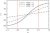 |
Fig. A.1 Observed barycenter shift as a function of real shift of the star in the focal plane, in arcseconds. Vertical red lines show the slit limits. The slit width is one arcsec. Three examples are shown: seeing much better than (0.5 arcsec), comparable to (1 arcsec), and larger than (2 arcsec) slit width. |
All Tables
All Figures
|
Fig. 1 Description of the geometry of the stars and spectrograph slit during the first observation: the observed difference in radial velocity between the stars depends on their true difference in RV and on their separation in the sky. |
| In the text | |
|
Fig. 2 As in Fig. 1, but now the slit has been rotated by 180 degrees. The measured difference in radial velocity between Figs. 1 and 2 will depend on the projected separation of the stars along the dispersion. |
| In the text | |
|
Fig. 3 Spectra HD 188088 for different slit angles. The lines of the two stars are clearly separated in the spectra. |
| In the text | |
|
Fig. 4 Example of cross-correlation function (black line) and fit (red line) for our observations. |
| In the text | |
|
Fig. 5 Optical design of a simple device to simultaneously record spectra with 180 degree orientation. The design is optimized for the UVES spectrograph. The rays with different colors do not represent different wavelengths, rather the geometrical position of the extremes, to show visually how the green ray, which is located at the upper limit at the entrance, and the blue ray, which is located at the lower extreme, maintain the geometry in slit 1 while they are geometrically rotated in slit 2, after an odd number of reflections. |
| In the text | |
|
Fig. A.1 Observed barycenter shift as a function of real shift of the star in the focal plane, in arcseconds. Vertical red lines show the slit limits. The slit width is one arcsec. Three examples are shown: seeing much better than (0.5 arcsec), comparable to (1 arcsec), and larger than (2 arcsec) slit width. |
| In the text | |
Current usage metrics show cumulative count of Article Views (full-text article views including HTML views, PDF and ePub downloads, according to the available data) and Abstracts Views on Vision4Press platform.
Data correspond to usage on the plateform after 2015. The current usage metrics is available 48-96 hours after online publication and is updated daily on week days.
Initial download of the metrics may take a while.