| Issue |
A&A
Volume 573, January 2015
|
|
|---|---|---|
| Article Number | A67 | |
| Number of page(s) | 11 | |
| Section | Numerical methods and codes | |
| DOI | https://doi.org/10.1051/0004-6361/201424741 | |
| Published online | 18 December 2014 | |
Inversion of stellar fundamental parameters from ESPaDOnS and Narval high-resolution spectra ⋆
1
Université de Toulouse, UPS-Observatoire Midi-Pyrénées, IRAP,
31400
Toulouse,
France
e-mail:
This email address is being protected from spambots. You need JavaScript enabled to view it.
2
CNRS, Institut de Recherche en Astrophysique et Planétologie,
14 av. É. Belin,
31400
Toulouse,
France
Received: 4 August 2014
Accepted: 10 November 2014
Abstract
The general context of this study is the inversion of stellar fundamental parameters from high-resolution Echelle spectra. We aim at developing a fast and reliable tool for the post-processing of spectra produced by ESPaDOnS and Narval spectropolarimeters. Our inversion tool relies on principal component analysis. It allows reducing dimensionality and defining a specific metric for the search of nearest neighbours between an observed spectrum and a set of observed spectra taken from the Elodie stellar library. Effective temperature, surface gravity, total metallicity, and projected rotational velocity are derived. Various tests presented in this study that were based solely on information coming from a spectral band centred on the Mg i b-triplet and had spectra from FGK stars are very promising.
Key words: astronomical databases: miscellaneous / methods: data analysis / stars: fundamental parameters
Based on observations obtained at the Télescope Bernard Lyot (TBL, Pic du Midi, France), which is operated by the Observatoire Midi-Pyrénées, Université de Toulouse, Centre National de la Recherche Scientifique (France) and the Canada-France-Hawaii Telescope (CFHT) which is operated by the National Research Council of Canada, CNRS/INSU and the University of Hawaii (USA).
© ESO, 2014
1. Introduction
This study is concerned with the inversion of fundamental stellar parameters from the analysis of high-resolution Echelle spectra. We focus on data collected since 2006 with the Narval spectropolarimeter mounted on the 2 m aperture Télescope Bernard Lyot (TBL) located at the summit of the Pic du Midi de Bigorre (France) and on data collected since 2005 with the ESPaDOnS spectropolarimeter mounted on the 3.6 m aperture CFHT telescope (Hawaii). We investigate, in particular, the capabilities of the principal component analysis (hereafter PCA) for setting up a fast and reliable tool to invert of stellar fundamental parameters from these high-resolution spectra.
The inversion of stellar fundamental parameters for each target that was observed with both Narval and ESPaDOnS spectropolarimeters constitutes an essential step towards (i) the subsequent post-processing of the data such as extracting polarimetric signals (see e.g., Paletou 2012 and references therein), but also (ii) exploring, or “data mining”, of the full set of data accumulated over the past eight years. In Sect. 2, we briefly describe the actual content of this database1.
The PCA has been used for stellar spectral classification since Deeming (1964). It has been in use since, and more recently for the purpose of inverting stellar fundamental parameters from the analysis of spectra of various resolutions. It is most often used together with artificial neural networks, however (see e.g., Bailer-Jones 2000; Re Fiorentin et al. 2007). The PCA is used there to reduce the dimensionality of the spectra before working on a multi-layer perceptron, which in turn allows linking input data to stellar parameters.
Our usage of the PCA for the inversion process is strongly influenced by this routinely made in solar spectropolarimetry in the past decade after the pioneering work of Rees et al. (2000). Very briefly, the reduction of dimensionality allowed by the PCA is directly used to build a specific metric from which a nearest-neighbour(s) search is made between an observed data set and the content of a training database. The latter can be made of synthetic data generated from input parameters that properly cover the a priori range of physical parameters expected to be deduced from the observations themselves. A quite similar use of PCA was also presented to classify and estimate of redshift of galaxies by Cabanac et al. (2002). However, in this study we use observed spectra from the Elodie stellar library as our reference data set (Prugniel et al. 2007). These spectra have for instance been used in a recent study related to the determination of atmospheric parameters of FGKM stars in the Kepler field (Molenda-Żakowicz et al. 2013). Fundamental elements of our method are described in Sect. 3. Its main originality relies also on simultaneously inverting the effective temperature Teff, the surface gravity log g, the metallicity [Fe/H], and the projected rotational velocity vsini directly and only from a specific spectral band extracted from the full range covered by ESPaDOnS and Narval.
Compared with alternative methods such as χ2 fitting to a library of (synthetic) spectra, as done by Munari et al. (2005) to analyse the RAVE survey, for instance, the main advantages of the PCA are that it reduces dimensionality – a critical issue when dealing with high-resolution spectra that cover a very broad bandwith. This allows a very fast processing of the data. Another advantage is the denoising of the original data (see e.g., Bailer-Jones et al. 1998 or Paletou 2012 in another context though). The PCA also differs from the projection method Matisse, which uses specific projection vectors that are attached to each stellar parameter that is to be inverted (Recio-Blanco et al. 2006). In that frame, these vectors are derived after assuming that they are linear combinations of every item belonging to a learning database of synthetic spectra.
In this study we restrict ourselves, on purpose, to a spectral domain ranging from 500 to 540 nm, that is, around the Mg i b-triplet lines. The main argument in favour of this spectral domain is that the spectral lines of this triplet are excellent surface gravity indicators (e.g., Cayrel & Cayrel 1963; Cayrel de Strobel 1969), log g being at the same time the most difficult parameter to retrieve from spectral data. It is also a spectral domain devoid of telluric lines. More recently, Gazzano et al. (2010) performed a convincing spectral analysis of Flames/Giraffe spectra working with a similar spectral domain. However, in our study we used observed spectra as the training database for our PCA-based inversion method.
Preliminary tests made by inverting spectra taken from the S4N survey (Allende Prieto et al. 2004) are discussed in Sect. 4. Finally, we proceed with inverting 140 spectra of FGK stars form PolarBase for which fundamental parameters are already available from the Spocs catalogue of Valenti & Fisher (2005).
2. Sources of data
Our reference spectra are taken from the Elodie stellar library (Prugniel et al. 2007; Prugniel & Soubiran 2001). They are publicly available2 and fully documented. The wavelength coverage of Elodie spectra is about 390–680 nm. This, unfortunately, prevents us from testing in the spectral domain at the vicinity of the infrared triplet of Ca ii, for instance (see e.g., Munari 1999 for a detailed case concerning this spectral range). We also used the high-resolution spectra at ℛ ~ 42 000.
First tests of our method were made with stellar spectra from the Spectroscopic Survey of Stars in the Solar Neighbourhood, also known as S4N (Allende Prieto et al. 2004). They are also publicly3 available and fully documented. The wavelength coverage is 362–1044 nm (McDonald Observatory, 2.7 m telescope) or 362–961 nm (La Silla, 1.52 m telescope), and the spectra have a resolution ℛ ~ 50 000.
However, our main purpose is inverting of stellar parameters from high-resolution spectra coming from Narval and ESPaDOnS spectropolarimeters. These data are now available from the public database PolarBase (Petit et al. 2014). Narval is a modern spectropolarimeter operating in the 380–1000 nm spectral domain, with a spectral resolution of 65 000 in its polarimetric mode. It is an improved copy, adapted to the 2 m TBL telescope, of the ESPaDOnS spectropolarimeter, which is in operations since 2004 at the 3.6 m aperture CFHT telescope.
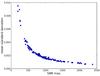 |
Fig. 1 Typical domain of variation of the noise level associated with the ESPaDOnS-Narval spectra that we process here. The mean standard deviation of noise per pixel for the wavelength range around the b-triplet of Mg i is displayed here vs. the highest signal-to-noise ratio (SNR) of the full spectra. |
PolarBase is operational since 2013. It is at the present time the largest on-line archive of high-resolution polarization spectra. It hosts data that were taken at the 3.6 m CFHT telescope since 2005 and with the 2 m TBL telescope since 2006. So far, more than 180 000 independent spectra are available for more than 2 000 distinct targets all over the Hertzsprung-Russell diagram. More than 30 000 polarized spectra are also available, mostly for circular polarization. Linear polarization data are still very rare and amount to a about 2% of the available data.
At present, the PolarBase database provides only Stokes I or V/Ic spectra calibrated in wavelength. Stokes I data are either normalized to the local continuum or not. We have plans to propose higher-level data however, such as pseudo-profiles resulting from line addition and/or least-squares deconvolution (see e.g., Paletou 2012), activity indexes and stellar fundamentals parameters. These last, in addition to being obviously interesting in themselves, is also indispensable for any accurate subsequent post-processing of these high-resolution spectra. These spectra also generally have high signal-to-noise ratio, as can be seen in Fig. 1. The Stokes I spectra we used result from combining four successive exposures, each of them carrying two spectra of orthogonal polarities generated by a Savart plate-type analyser. This procedure of double “beam-exchange” measurement is designed for the purpose of extracting (very) weak polarization signals (see e.g., Semel et al. 1993).
3. PCA-based inversion
Our PCA-based inversion tool is strongly inspired by magnetic and velocity field inversion tools that have been developed in the past decade to diagnose solar spectropolarimetric data (see e.g., Rees et al. 2000). Improvements of this method have recently been reported by Casini et al. (2013), for instance. Below we describe its main characteristics in the particular context of our study.
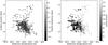 |
Fig. 2 Graphical summary of the coverage in stellar parameters corresponding to the content of our Elodie spectra training database (for FGK stars). Note that we adopted values of vsini from the Vizier at CDS catalogue III/244 (Głebocki & Gnaciński 2005). Size and colour of each dot are proportional to either [Fe/H] (left) or vsini (right). |
3.1. Training database
Our training database was created after the Elodie stellar spectral library (Prugniel et al. 2007; Prugniel & Soubiran 2001; see also the Vizier at CDS catalogue III/251). Stellar parameters associated with each spectrum were extracted by us from the CDS, using ressources from the Python package astroquery4, in particular the components allowing queries of Vizier catalogues.
We complemented this information with a value of the projected rotational velocity for each object and spectrum of our database. To do so, we queried the catalogue of stellar rotational velocities of Głebocki & Gnaciński (2005, also Vizier at CDS catalogue III/2445). Moreover, we removed all objects for which we could not find a value of vsini in this catalogue.
Since our preliminary tests concerns the inversion of the S4N survey as well as objects in common of PolarBase and of the Spocs catalogue (Valenti & Fisher 2005), we limited ourselves to spectra for which Teff lies between 4000 and 8000 K, log g is greater than 3.0 dex, and [Fe/H] is greater than − 1.0 dex. We also had to reject a few Elodie spectra that we found to be unproperly corrected for radial velocity and therefore misaligned in wavelength with respect to the other spectra. The various coverage in stellar parameters from the finally 905 selected spectra are summarized in Figs. 2.
Finally, following Muñoz Bermejo et al. (2013), we adopted the same renormalization procedure, homogeneously, for the whole set of Elodie spectra that were our training database. It is an iterative method consisting of two main steps. The first stage consists of fitting the normalized flux in the spectral bandwith of interest by a high-order (eight) polynomial. Then we computed D(λ) that is the difference between the initial spectra and the polynomial fit and its mean  and standard deviation σD. We rejected wavelengths where
  were either lower than − 0.5σD or above 3σD. This scheme was iterated ten times, which guarantees that we properly extracted the continuum envelope of the initial spectra. Finally, we use the remaining flux values to renormalize the initial spectra. As Fig. 3 shows, this concerns relatively small corrections of the continuum level that never exceed a few percent. As mentioned earlier by Muñoz Bermejo et al. (2013), this procedure may be debatable, but we found it satisfactory, and it was consistently applied to all the spectra we used.
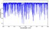 |
Fig. 3 Typical example of the continuum level fit (strong dark line) on top of the original spectrum that still has small normalization errors that need to be corrected for. |
3.2. Reduction of dimensionality
The ESPaDOnS and Narval spectropolarimeters typically provide about 250 000 flux measurements vs. wavelength across a spectral range spanning from about 380 to 1000 nm for each spectrum. We only consider spectra obtained in the polarimetric mode at a resolvance of ℛ ~ 65 000. One of our main objective is to use stellar parameters derived from Stokes I spectra directly for the subsequent post-processing of the multi-line polarized spectra that are obtained simultaneously (see e.g., Paletou 2012 and references therein).
We adopted a first reduction of dimensionality by restricting the spectral domain from which we inverted stellar parameters to the vicinity of the Mg i b-triplet, that is for wavelengths ranging from 500 to 540 nm. Good surface gravity indicators such as the strong lines of the b-triplet of Mg i (λλ 516.75, 517.25, and 518.36 nm) an those of several other metallic lines in their neighbourood, and the absence of telluric lines in this spectral domain are the main arguments we used. The matrix S that represents our training database size is Nspectra = 905 by Nλ = 8 000.
Next, we computed the eigenvectors ek(λ) of the variance-covariance matrix defined as 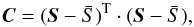 (1)where
  is the mean of S along the Nspectra-axis. Therefore C is an Nλ × Nλ matrix. In the framework of the PCA reduction of dimensionality is reduced by representing the original data with a limited set of projection coefficients
 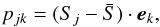 (2)with kmax ≪ Nλ. For the processing of all observed spectra, we adopted kmax = 12.
The most frequent argument supporting the choice of kmax relies on the accuracy achieved for reconstructing the original set of Si’s from a limited set of eigenvectors (see e.g., Rees et al. 2000 or Muñoz Bermejo et al. 2013). In the present case, we display in Fig. 4 the mean reconstruction error 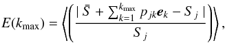 (3)as a function of the maximum number of eigenvectors considered for computing the projection coefficients p. Figure 4 shows that this reconstruction error is better than 1% for kmax ≥ 12. In addition, at the same rank, an alternative estimator such as the cumulative sum of the ordered eigenvalues normalized to their sum becomes higher than 0.95.
 |
Fig. 4 Reconstruction error as a function of the number of eigenvectors used for computing of the projection coefficients p. The mean reconstruction error drops below 1% (with a standard deviation of 0.4%) after rank 12. The right-hand scale shows the cumulative sum of the ordered eigenvalues normalized to their sum (⋆). |
To conclude this part, we display in Fig. 5 the 12 eigenvectors that we used below.
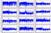 |
Fig. 5 From top left to bottom right, the 12 eigenvectors used in our inversion method. Each of them is displayed vs. the same wavelength scale in nm. |
3.3. Nearest-neighbour(s) search
The above described reduction of dimensionality allows performing a fast and reliable inversion of observed spectra, after they have been (i) corrected for the wavelength shift vs. the spectra in our database, because of the radial velocity of the target; (ii) continuum-renormalized as accurately as possible; (iii) degraded in spectral resolution to be similar to the ℛ ~ 42 000 resolvance of the Elodie spectra we use and; finally (iv) resampled in wavelength like the collection of Elodie spectra. We return to these various stages in the next section. After these tasks have been achieved, the inversion process is the following:
O(λ) denotes the observed spectrum made similar to those of Elodie. We now compute the set of projection coefficients 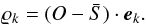 (4)The nearest-neighbour search is made by seeking the minimum of the squared Euclidian distance
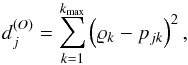 (5)where j spans the number, or a limited number if any a priori is known about the target, of distinct reference spectra in the training database. In practice, we did not limit ourselves to the nearest-neighbour search, although it already provides a relevant set of stellar parameters. Because PCA-distances between several neighbours may be of the same order, we adopted a simple procedure that consists of considering all neighbours in a domain
 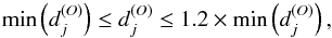 (6)and derived stellar parameters as the (simple) mean of each set of parameters {Teff; log g; [Fe/H]; vsini} that characterises this set of nearest neighbours (A. López Ariste, priv. comm.). No significant changes in the results were recorded either for a smaller range of PCA-distances or when adopting, for example, distance-weighted mean parameters. This point is discussed again below.
3.4. Internal error
To characterise our inversion method, we inverted the stellar parameters Teff, log g, [Fe/H] and vsini, for every spectrum (905) that constitutes the training database. However, at each step we removed the spectra that were processed from the database (and then recomputed the eigenvalues and eigenvectors of the new variance-covariance matrix).
Bias and standard deviation of the differences between inverted Elodie spectra and their initial stellar parameters of reference Teff (K), log g, [Fe/H] (dex), and vsini (km s-1).
To summarize this analysis, we list in Table 1 the internal errors, σ, measured for each inverted stellar parameter. The disappointing result on vsini mainly comes from a suspicious scatter of results for these objects with large vsini, typically beyond 100 km s-1. However, for our tests with S4N and PolarBase data, we did not have to work with objects with vsini beyond 80 km s-1 (see next sections).
4. Inversion of S4N spectra
A convincing test of our method would be to invert high-resolution spectra that were gathered in the frame of the S4N spectroscopic survey (Allende Prieto et al. 2004).
We only selected the S4N spectra for which all three parameters {Teff; log g; [Fe/H]} have been determined by Allende Prieto et al. (2004). We used the same reference catalogue as the one used for the Elodie spectra to add a vsini value to each spectrum (see e.g., Paletou & Zolotukhin 2014). Since they were acquired at a higher spectral resolution than those of Elodie, we adapted each spectrum to the resolvance of Elodie of ℛ ~ 42 000 using an appropriate Gaussian filter. Finally we applied the same renormalization procedure to all spectra as was applied to our Elodie spectra database.
We identified 49 objects in common between S4N and our sample of 905 objects taken from the Elodie stellar library. Using the catalogue values for effective temperature Teff, surface gravity log g, and metallicity [Fe/H], we easily estimated the bias and standard deviations between the two distinct estimate for each stellar parameter. The results are summarized in Table 2.
Bias and standard deviation of the absolute differences between reference stellar parameters Teff (K), log g (dex), and [Fe/H] (dex) retrieved from the S4N and the Elodie catalogues for the 49 objects in common between our data samples.
These results were then compared with the results of our inversion of 104 S4N spectra using our Elodie training database for PCA. They are summarized, for each stellar parameter including vsini in Fig. 6 and Table 3 (where we also detail specific values for the inverted spectra of the 49 objects in common between S4N and our Elodie sample and the 55 remaining objects). Bias and dispersions, especially conspicuous for log g, measured after our inverted parameters appear to be quite direct imprints of the discrepancies that were already clear from the direct comparison between the reference values for objects in common between the two samples. However, taking into account that our inversion only relies on spectroscopic information from a limited (but relevant) spectral band, we find our approach satisfactory for our purpose.
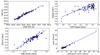 |
Fig. 6 Stellar fundamental parameters inverted from the analysis of S4N spectra, using our PCA-Elodie method vs. their S4N catalogue values of reference (except for vsini – see text). The bias and standard deviation deduced from the analysis of the difference between inverted and catalogue and reference parameters are (− 74; 115) for Teff, (0.16; 0.16) for log g and (− 0.01; 0.11) for [Fe/H]. For vsini values for which the source of data is not the S4N catalogue, however, we find (− 0.36; 1.61). |
Our method also allows a reliable and direct inversion of the projected rotational velocity vsini of stars, without any other limitation than the one coming from the limit in vsini attached to the identified values for spectra present in our Elodie training database – see Figs. 2, for example. Using synthetic spectra (computed for hypothetical non-rotating stars), Gazzano et al. (2010) were limited to stars with a vsini lower than about 11 km s-1, for instance. In our case, we accurately retrieved vsini values up to the most extreme case of ~80 km s-1 in our sample that is, the high-proper motion F1V star HIP 779526 that is, fast rotators for which usual synthetic models are unsatisfactory.
Another advantage of our method is that nearest-neighbour(s) are also identifiable as objects that is, as other stars. In that sense, our method can also be seen as relevant for classification. For instance, considering the only objects in common between our S4N and our Elodie spectra and objects sample, in 75% of the cases the very nearest neighbour is another spectrum of the same object and, for the remainder, conditions expressed in Eq. (6) guarantee that the same object spectrum belongs to the set of nearest neighbours.
5. Inversion of PolarBase spectra
Below we first discuss details of the kind of conditioning that has to be applied to PolarBase spectra to make them similar to our Elodie-based training database. Then we discuss the inversion of solar spectra taken on reflection over the Moon surface at the TBL telescope, and finally inversions of 140 spectra from FGK objects in common with the sample studied by Valenti & Fischer (2005).
5.1. Conditioning of PolarBase spectra
The first and obvious task to perform on observed spectra is to correct for their wavelength shift vs. Elodie spectra, which are found already corrected for radial velocity (vrad). The radial velocity of the target at the time of the observation is deduced from the centroid, in a velocity space, of the pseudo-profile resulting from the addition (see e.g., Paletou 2012) of the three spectral lines of the Ca ii infrared triplet whose rest wavelengths are 849.802, 854.209 and 866.214 nm. This can be done with any other set of spectral lines assumed to be a priori present in the spectra we wish to process. One of the advantages of the Ca ii infrared triplet is its persistence for spectral types ranging from A to M. When vrad is known, the observed profile is set on a new wavelength grid, at rest.
We checked with a solar spectrum (see also the next section) that vrad have to be known to an accuracy of the order of δv/ 4 with δv = c/ ℛ i.e., about 1.15 km s-1 with our ESPaDOnS-Narval data. Beyond this value, estimates of Teff and vsini first start to be significantly affected by the misalignement of the observed spectral lines with those of the spectra of the training database. Indeed, the neighbourhood identified by our PCA-based approach can change quite dramatically because of such a spectral misalignement.
A second step consists of adapting the resolution of the initial spectra, about ℛ ~ 65 000 in the polarimetric mode, to the resolution of the training database spectra that is, ℛ ~ 42 000. This is done by convolving the initial observed profile by a Gaussian profile of adequate width. Then we resampled the wavelength grid down to the one common to all reference spectra and we interpolated the original spectra onto the new wavelength grid. Finally, we applied the same renormalization procedure as decribed in Sect. 3.1, for consistency.
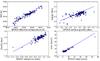 |
Fig. 7 Stellar fundamental parameters inverted from PolarBase spectra in common with the Spocs catalogue, using our PCA-Elodie method vs. Spocs reference values, including vsini. Respective bias and standard deviation deduced from the analysis of the difference between inverted and reference parameters are (23; 115) for Teff, (0.10; 0.19) for log g, (0.02; 0.10) for [Fe/H], and (− 0.04; 1.68) for vsini. |
5.2. Solar spectra observed with Narval
First tests of our inversion method with PolarBase data were performed using solar spectra observed by the 2 m aperture TBL telescope by reflection over the surface of the Moon in March and June 2012.
Using the very same training database as was used for the tests done with S4N data, we identified as nearest-neighbour star to the Sun HD 186427 (also known as 16 Cyg B). It is a G3V planet-hosting star often identified as a solar twin (see e.g., Porto de Mello et al. 2014). Its stellar fundamental parameters are Teff = 5757 K, log g = 4.35 dex, [Fe/H] = 0.06, and vsini ~ 2.18 km s-1 (see also Tucci Maia et al. 2014, for a recent determination of these parameters). The other nearest neighbour we identified is HD 29150, a star whose main parameters are Teff = 5733 K, log g ~ 4.35 dex (Lee et al. 2011, from Simbad at CDS query), [Fe/H] = 0.0, and vsini ~ 1.8 km s-1.
Taking into consideration this neighbourhood, in the PCA-sense, we thus derived quite satisfactory estimates for the effective temperature Teff = 5745 K, surface gravity log g = 4.35 dex, a metallicity of [Fe/H] = 0.03, and vsini ~ 2 km s-1 typical of the (very) slowly rotating Sun, as observed by reflection over the Moon surface with the Narval at TBL spectropolarimeter.
This is quite consistent with the test consisting of inverting solar spectra taken from the Elodie stellar library, but not a member of our training database. In this case, we recover neighbours 16 Cyg B and HD 29150 plus the additional HD 146233 (also known as 18 Sco) and HD 42807, a RS CVn star of G2V type, also very similar to the Sun.
Bias and standard deviation of the absolute differences between stellar parameters Teff (K), surface gravity log g, metallicity [Fe/H] (dex), and projected rotational velocity vsini (km s-1) obtained from the Spocs catalogue of Valenti & Fischer (2005, reference values) and our inversion method using Elodie spectra.
5.3. Other FGK stars
We identified in the present content of PolarBase 140 targets that are also identified in the Spocs catalogue. For our next tests of our method, we selected the spectra with the best signal-to-noise ratio for every object. Typical values were already given in Fig. 1.
Results and characterization of our inversion are given in Table 4 and with more details in Fig. 7. This figure also gives an idea about the range of variations of parameters that are expected for the set of spectra and objects that are studied here. Overall, the figures are quite similar to those obtained with the S4N, although bias values for Teff and log g are lower for the Spocs data.
5.3.1. Effective temperature
Ths standard deviation on the differences between our values and those of the Spocs reference is the same as the difference we evaluated from S4N spectra (see Table 3). However, the bias value of 23 K is much lower for this sample of objects and PolarBase spectra. We note also that the most important dispersion is for the coolest objects of our sample with a Teff of about 5000 K.
A more detailed inspection of outliers in effective temperature, taking into account alternative and more recent estimates of Teff than the estimate adopted from Spocs, reveals that the most extreme ΔTeff we identified are quite often overestimated. This is for instance the case for the K1V star LHS 44, for which a recent determination by Maldonado et al. (2012) is +200 K higher than that of Valenti & Fischer (2005) and only 140 K higher than ours. Another effect may also come from new estimates of parameters for Elodie objects themselves, an issue we shall discuss below.
Our estimates of the effective temperature from spectropolarimetric data are satisfactory and can be used in selecting a proper mask (i.e., at least a list of spectral lines) that will be, in turn, used for the subsequent extraction of polarized signatures.
5.3.2. Surface gravity
It is well known that surface gravity is the most difficult parameter to extract from the analysis of spectroscopic data. The most conspicuous outliers are quite easily detected on the log g subplot in Fig. 7. The top three of them, which show Δlog g ~ 0.5 dex or higher, we find EK Dra, LTT 8785 and HD 22918. For EK Dra, our estimate of log g ~ 3.6 dex is much too low compared with the (rare) values found in the litterature (~4.5 dex). This may be compensated by the fact that its identified nearest-neighbour star is the G2IV subgiant HD 126868 (also known as 105 Vir), for which log g = 3.6 dex in the Elodie catalogue, although a value of 3.9 dex is reported elsewhere (see e.g., the Pastel catalogue: Soubiran et al. 2010). For LTT 8785 and HD 22918, an examination of alternative estimates for log g (e.g., Massarotti et al. 2008; Jones et al. 2011) shows that Spocs values may have been slightly overestimated. In addition, the surface gravity (log g ~ 3.23) of the nearest neighbour (and the same object in both cases) HD 42983 may have been underestimated. An inspection of Vizier at CDS for this object indicates four different estimates ranging from 3.23 to 3.6 with a median value of 3.5. Taking this into account, Δlog g does not exceed 0.2 dex between our inverted values and reference ones, which is satisfactory.
5.3.3. Metallicity
We now inspect our results for metallicity. First of all, we included LHS 44 in our sample, which has [Fe/H] = − 1.16 according to Valenti & Fischer (2005), a value a priori excluded from our working range. But our inversion method still indicates these objects in our sample as bearing the lowest [Fe/H] values. Then by decreasing order of Δ[Fe/H] of our inverted values and the reference values, we find HD 30508, 40 Eri, and LHS 3976. We found a systematically better agreement between our estimate and statistics on all data available at Vizier, to within 0.05 dex.
5.3.4. Projected rotational velocity
Our determinations of vsini are correct and especially interesting for objects with a significant projected rotational velocity, for example, greater than about 10 km s-1. The main outlier, as seen in Fig. 7, is HR 1817, for which we derive a vsini ~ 43 km s-1 while the Spocs value is about 55 km s-1. It is a F8V RS CVn star that is also known as AF Lep, for which another value of 52.6 km s-1, still about 10 km s-1 greater than our estimate, was more recently published by Schröder et al. (2009).
Other methods for determining vsini already exist. However, to the best of our knowledge, they require a template (synthetic) spectrum at vsini ~ 0 or, at least, a list of spectral lines a priori expected in the spectra, as auxilliary and support data (see e.g., Díaz et al. 2011 and references therein). Data-processing tools that we attach to PolarBase will therefore include a complementary Fourier analysis module providing an additional vsini determination, once stellar fundamental parameters will be available from our inversion tool7. Note also that with our PCA-based method, we are mostly interested in the intermediate vsini regime, that is between 10 and 100 km s-1. Indeed, for slower rotators for which rotational broadening becomes of the order of other sources of broadening (e.g., instrumental or turbulent), a more detailed or specific line profile analysis may be required.
6. Discussion
As briefly remarked earlier, the fact that the current implementation of our method relies on observed data makes it also somewhat relevant to classification. Indeed, we did not only identify nearest spectra since nearest neighbour(s) can also be identified as objects that is, as other stars. This important fact is also totally independent of the method used to determine the stellar parameters for these objects.
Therefore, unless modifying the sample of spectra and objects that constitute our training database, we do not expect any change in the relation between inverted spectra and nearest neighbours as objects, even though evaluations of their various stellar parameters may still change in time. Another interesting point is that this is also true for any other stellar parameter – especially those contributing to the spectral signature of a star, beyond the limited set of fundamental parameters we considered in this study.
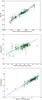 |
Fig. 8 Stellar fundamental parameters and their respective uncertainties inverted from PolarBase spectra in common with the Spocs catalogue, obtained using our PCA-Elodie method vs. Spocs reference values. These values were deduced from all determinations for each nearest neighbour compiled in the Pastel catalogue of Soubiran et al. (2010). |
Values and uncertainties of the inverted stellar parameters Teff, log g, and [Fe/H] for Spocs objects in common with PolarBase using our Elodie-based PCA method.
Taking advantage of this, instead of using values given by the Elodie catalogue alone, for each Spocs spectra we analysed, we gathered for every nearest neighbour all the evaluations of effective temperature, surface gravity, and metallicity provided by the comprehensive Pastel catalogue8 (Soubiran et al. 2010). We also evaluated uncertainties on each fundamental parameter as the standard deviation of the full set of collected values, except for the unavailable projected rotational velocity. The results are displayed in Figs. 8, and details are given in Table 5. Mean errors given in Table 5 are 110 K, 0.16 dex and 0.09 dex for Teff, log g and [Fe/H] respectively which is quite consistent, but slightly better than the standard deviation values already given in Table 4.
As a final remark, it is also worth mentioning that although we used it together with a training database made of observed spectra, our PCA-based inversion method can be equally implemented using synthetic spectra.
7. Conclusion
We have implemented a fast and reliable PCA-based numerical method for inverting stellar fundamental parameters Teff, log g, and [Fe/H] and, the projected rotational velocity vsini, from the analysis of high-resolution Echelle spectra delivered by the Narval and ESPaDOnS spectropolarimeters. First tests, mainly made with FGK-star spectra, show a good agreement between our inverted stellar parameters and reference values published by Allende Prieto et al. (2004) and Valenti & Fischer (2005). We also believe that our method will also be efficient for analysing spectra from cooler M stars as well as from hotter stars, up to spectral type A.
We used it, so far, with a spectral band located at the vicinity of the b-triplet of Mg i and without any help from additional (e.g., photometric) information, which is particularly challenging. However, we can easily either extend or change the spectral domain of use, or combine analyses from several distinct spectral domains to further constrain and refine the stellar parameters determination. In that respect, it is important to realize that PCA allows for a quite dramatic reduction of dimensionality, of the order of 800 (~Nλ/kmax) for the configuration we presented here. This capability is indeed of great interest for a comprehensive post-processing of high-resolution spectra covering a very broad bandwidth such as those from the ESPaDOnS and Narval spectropolarimeters.
polarbase.irap.omp.eu
hebe.as.utexas.edu/s4n/
astroquery.readthedocs.org
We had to correct the value of 25 km s-1 given for HD 16232 because it is significantly underestimated compared with alternative determinations (with a median of 40 km s-1).
Note that for this object, five estimates of vsini from Vizier at CDS can be identified that range from 70 to 90 km s-1, but whose median value of 75 km s-1 agrees very well with our own estimate.
The same is true for the refinement of radial velocity measurements, which can be improved by line addition when a proper list of expected spectral line wavelengths (at rest) is identified.
For four targets for which we could not retrieve data from Pastel, we instead used instead their TGMET values (Katz et al. 1998) that are also available from the Elodie at Vizier catalogue.
Acknowledgments
This research has made use of the VizieR catalogue access tool, CDS, Strasbourg, France. The original description of the VizieR service was published in A&AS 143, 23. This research has made use of the SIMBAD database, operated at CDS, Strasbourg, France. PolarBase data were provided by the OV-GSO (ov-gso.irap.omp.eu) datacenter operated by CNRS/INSU and the Université Paul Sabatier, Observatoire Midi-Pyrénées, Toulouse (France).
References
- Allen de Prieto, C., Barklem, P. S., Lambert, D. L., & Cunha, K. 2004, A&A, 420, 183 [NASA ADS] [CrossRef] [EDP Sciences] [Google Scholar]
- Bailer-Jones, C. A. L. 2000, ApJ, 357, 197 [Google Scholar]
- Bailer-Jones, C. A. L., Irwin, M., & von Hippel, T. 1998, MNRAS, 298, 361 [NASA ADS] [CrossRef] [Google Scholar]
- Cabanac, R. A., de Lapparent, V., & Hickson, P. 2002, A&A, 389, 1090 [NASA ADS] [CrossRef] [EDP Sciences] [Google Scholar]
- Casini, R., Asensio Ramos, A., Lites, B. W., & López Ariste, A. 2013, ApJ, 773, 180 [NASA ADS] [CrossRef] [Google Scholar]
- Cayrel, G., & Cayrel, R. 1963, ApJ, 137, 431 [NASA ADS] [CrossRef] [Google Scholar]
- Cayrel de Strobel, G. 1969, in Proc. of the 3rd Harvard-Smithsonian Conf. on Stellar Atmospheres, ed. O. Gingerich, 35 [Google Scholar]
- Deeming, T. J. 1964, MNRAS, 127, 493 [NASA ADS] [Google Scholar]
- Díaz, C. G., González, J. F., Levato, H., & Grosso, M. 2011, A&A, 531, A143 [NASA ADS] [CrossRef] [EDP Sciences] [Google Scholar]
- Gazzano, J.-C., de Laverny, P., Deleuil, M., et al. 2010, A&A, 523, A91 [NASA ADS] [CrossRef] [EDP Sciences] [Google Scholar]
- Głebocki, R., & Gnaciński, P. 2005, VizieR On-line Data Catalog: III/244 [Google Scholar]
- Jones, M. I., Jenkins, J. S., Rojo, P., & Melo, C. H. F. 2011, A&A, 536, A71 [NASA ADS] [CrossRef] [EDP Sciences] [Google Scholar]
- Katz, D., Soubiran, C., Cayrel, R., Adda, M., & Cautain, R. 1998, A&A, 338, 151 [NASA ADS] [Google Scholar]
- Lee, Y.S., Beers, T.C., Allen de Prieto, C., et al. 2011, AJ, 141, 90 [NASA ADS] [CrossRef] [Google Scholar]
- Maldonado, J., Eiroa, C., Villaver, E., Montesinos, B., & Mora, A. 2012, A&A, 541, A40 [NASA ADS] [CrossRef] [EDP Sciences] [Google Scholar]
- Massarotti, A., Latham, D. W., Stefanik, R. P., & Fogel, J. 2008, AJ, 135, 209 [NASA ADS] [CrossRef] [Google Scholar]
- Molenda-Żakowicz, J., Sousa, S. G., Frasca, A., et al. 2013, MNRAS, 434, 1422 [NASA ADS] [CrossRef] [Google Scholar]
- Munari, U. 1999, Baltic Astron., 8, 73 [Google Scholar]
- Munari, U., Sordo, R., Castelli, F., & Zwitter, T. 2005, A&A, 442, 1127 [NASA ADS] [CrossRef] [EDP Sciences] [Google Scholar]
- Muñoz Bermejo, J., Asensio Ramos, A., & Allen de Prieto, C. 2013, A&A, 553, A95 [NASA ADS] [CrossRef] [EDP Sciences] [Google Scholar]
- Paletou, F. 2012, A&A, 544, A4 [NASA ADS] [CrossRef] [EDP Sciences] [Google Scholar]
- Paletou, F., & Zolotukhin, I. 2014 [arXiv:1408.7026] [Google Scholar]
- Petit, P., Louge, T., Théado, S., et al. 2014, PASP, 126, 469 [NASA ADS] [CrossRef] [Google Scholar]
- Porto de Mello, G. F., da Silva, R., da Silva, L., & de Nader, R. V. 2014, A&A, 563, A52 [NASA ADS] [CrossRef] [EDP Sciences] [Google Scholar]
- Prugniel, P., & Soubiran, C. 2001, A&A, 369, 1048 [NASA ADS] [CrossRef] [EDP Sciences] [Google Scholar]
- Prugniel, P., Soubiran, C., Koleva, M., & Le Borgne D. 2007 [arXiv:astro-ph/0703658] [Google Scholar]
- Recio-Blanco, A., Bijaoui, A., de Laverny, P., et al. 2006, MNRAS, 370, 141 [NASA ADS] [CrossRef] [Google Scholar]
- Rees, D. E., López Ariste, A., Thatcher, J., & Semel, M. 2000, A&A, 355, 759 [NASA ADS] [Google Scholar]
- Re Fiorentin, P., Bailer-Jones, C. A. L., Lee, et al. 2007, A&A, 465, 1373 [NASA ADS] [CrossRef] [EDP Sciences] [Google Scholar]
- Schröder, C., Reiners, A., & Schmitt, J. H. M. M. 2009, A&A, 493, 1099 [NASA ADS] [CrossRef] [EDP Sciences] [Google Scholar]
- Semel, M., Donati, J. F., & Rees, D. E. 1993, A&A, 278, 231 [NASA ADS] [Google Scholar]
- Soubiran, C., Le Campion, J.-F., Cayrel de Strobel, G., & Caillo, A. 2010, A&A, 515, A111 [NASA ADS] [CrossRef] [EDP Sciences] [Google Scholar]
- Tucci Maia, M., Meléndez, J., & Ramírez, I. 2014, ApJ, 790, L25 [NASA ADS] [CrossRef] [Google Scholar]
- Valenti, J. A., & Fischer, D. A. 2005, ApJS, 159, 141 [NASA ADS] [CrossRef] [MathSciNet] [Google Scholar]
All Tables
Bias and standard deviation of the differences between inverted Elodie spectra and their initial stellar parameters of reference Teff (K), log g, [Fe/H] (dex), and vsini (km s-1).
Bias and standard deviation of the absolute differences between reference stellar parameters Teff (K), log g (dex), and [Fe/H] (dex) retrieved from the S4N and the Elodie catalogues for the 49 objects in common between our data samples.
Bias and standard deviation of the absolute differences between stellar parameters Teff (K), surface gravity log g, metallicity [Fe/H] (dex), and projected rotational velocity vsini (km s-1) obtained from the Spocs catalogue of Valenti & Fischer (2005, reference values) and our inversion method using Elodie spectra.
Values and uncertainties of the inverted stellar parameters Teff, log g, and [Fe/H] for Spocs objects in common with PolarBase using our Elodie-based PCA method.
All Figures
|
Fig. 1 Typical domain of variation of the noise level associated with the ESPaDOnS-Narval spectra that we process here. The mean standard deviation of noise per pixel for the wavelength range around the b-triplet of Mg i is displayed here vs. the highest signal-to-noise ratio (SNR) of the full spectra. |
| In the text | |
|
Fig. 2 Graphical summary of the coverage in stellar parameters corresponding to the content of our Elodie spectra training database (for FGK stars). Note that we adopted values of vsini from the Vizier at CDS catalogue III/244 (Głebocki & Gnaciński 2005). Size and colour of each dot are proportional to either [Fe/H] (left) or vsini (right). |
| In the text | |
|
Fig. 3 Typical example of the continuum level fit (strong dark line) on top of the original spectrum that still has small normalization errors that need to be corrected for. |
| In the text | |
|
Fig. 4 Reconstruction error as a function of the number of eigenvectors used for computing of the projection coefficients p. The mean reconstruction error drops below 1% (with a standard deviation of 0.4%) after rank 12. The right-hand scale shows the cumulative sum of the ordered eigenvalues normalized to their sum (⋆). |
| In the text | |
|
Fig. 5 From top left to bottom right, the 12 eigenvectors used in our inversion method. Each of them is displayed vs. the same wavelength scale in nm. |
| In the text | |
|
Fig. 6 Stellar fundamental parameters inverted from the analysis of S4N spectra, using our PCA-Elodie method vs. their S4N catalogue values of reference (except for vsini – see text). The bias and standard deviation deduced from the analysis of the difference between inverted and catalogue and reference parameters are (− 74; 115) for Teff, (0.16; 0.16) for log g and (− 0.01; 0.11) for [Fe/H]. For vsini values for which the source of data is not the S4N catalogue, however, we find (− 0.36; 1.61). |
| In the text | |
|
Fig. 7 Stellar fundamental parameters inverted from PolarBase spectra in common with the Spocs catalogue, using our PCA-Elodie method vs. Spocs reference values, including vsini. Respective bias and standard deviation deduced from the analysis of the difference between inverted and reference parameters are (23; 115) for Teff, (0.10; 0.19) for log g, (0.02; 0.10) for [Fe/H], and (− 0.04; 1.68) for vsini. |
| In the text | |
|
Fig. 8 Stellar fundamental parameters and their respective uncertainties inverted from PolarBase spectra in common with the Spocs catalogue, obtained using our PCA-Elodie method vs. Spocs reference values. These values were deduced from all determinations for each nearest neighbour compiled in the Pastel catalogue of Soubiran et al. (2010). |
| In the text | |
Current usage metrics show cumulative count of Article Views (full-text article views including HTML views, PDF and ePub downloads, according to the available data) and Abstracts Views on Vision4Press platform.
Data correspond to usage on the plateform after 2015. The current usage metrics is available 48-96 hours after online publication and is updated daily on week days.
Initial download of the metrics may take a while.