| Issue |
A&A
Volume 572, December 2014
|
|
|---|---|---|
| Article Number | L7 | |
| Number of page(s) | 4 | |
| Section | Letters | |
| DOI | https://doi.org/10.1051/0004-6361/201424953 | |
| Published online | 28 November 2014 | |
The existence of the Λ effect in the solar convection zone as indicated by SDO/HMI data
Leibniz-Institut für Astrophysik Potsdam, An der Sternwarte 16, 14482 Potsdam, Germany
e-mail: gruediger@aip.de
Received: 10 September 2014
Accepted: 31 October 2014
The empirical finding with data from the Helioseismic and Magnetic Imager instrument onboard the Solar Dynamics Observatory of positive (negative) horizontal Reynolds stress at the northern (southern) hemisphere for solar giant cells is discussed for its consequences on the theory of solar/stellar differential rotation. By solving the nonlinear Reynolds equation for the angular velocity Ω when neglecting the meridional circulation, we show that the horizontal Reynolds stress of the northern hemisphere is always negative at the surface but positive in the bulk of the solar convection zone by the action of the Λ effect. The Λ effect, which describes the angular momentum transport of rigidly rotating anisotropic turbulence and which avoids a rigid-body rotation of the convection zones, is in the horizontal direction of cubic power in Ω and proves to be always positive (negative) in the northern (southern) hemisphere in both theory and simulations. In contrast, theories without the Λ effect, which may provide the observed solar rotation law only by the action of a meridional circulation, will lead to a horizontal Reynolds stress with signs that are not observed.
Key words: Sun: rotation / turbulence / convection
© ESO, 2014
1. Introduction
The differential rotation of the stellar surfaces which has currently been observed for many thousands of stars (Reinhold et al. 2013) demonstrates that there is a non-diffusive angular momentum transport in rotating convection zones. There are various transporters of angular momentum in a rotating turbulent fluid, such as the turbulence-induced Reynolds stress that transports angular momentum by its components ⟨ uruφ ⟩ and ⟨ uθuφ ⟩ in radial and in latitudinal directions1. Boussinesq (1897) and Taylor (1915) connected the one-point correlation tensor Qij = ⟨ ui(x,t)uj(x,t) ⟩, which is symmetric by definition in its indices i and j, with the shear of a large-scale flow U so that Qij = ... − νT(Ui,j + Uj,i) results with the positive-definite eddy viscosity νT. Here, the notation U + u as the turbulent velocity field with the background flow U and its fluctuation u has been introduced. This Boussinesq hypothesis, which does not reflect the anisotropies in the turbulence field, immediately yields 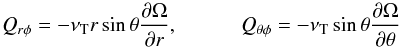 (1)for the mentioned cross-correlations as being caused by the non-uniformity of the angular velocity Ω of the global rotation. Since they vanish for rigid rotation, they cannot serve to maintain nonuniform rotation Ω = Ω(r,θ). The turbulence in a convection zone, however, is subject to a distinct radial anisotropy by the central gravity that questions the validity of the relations (1). With the concept of an anisotropic viscosity tensor, Kippenhahn (1963) derived a generalized linear relation for the radial transport, i.e.,
 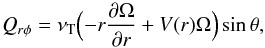 (2)where the second term in (1), however, remains unchanged. The sign of the new function V reflects the anisotropy in the turbulence, it vanishes for isotropic turbulence, and it is negative if on average the radial velocity component exceeds the horizontal one2.
Stationary solutions for the angular velocity have to fulfill the φ component of the Navier-Stokes equation in turbulent flows; i.e.,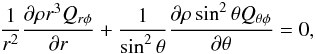 (3)which ensures the conservation of the angular momentum in the rotating turbulence when neglecting the mean meridional circulation and the molecular viscosity. Here, ρ is the density. Inserting (2) and the second term in (1) into (3), one finds Ω dependent on r but independent of θ. For positive radial shear in the rotation law, on the other hand, a meridional flow toward the equator is induced at the surface, which accelerates the equator by transporting angular momentum (Kippenhahn 1963). Such a meridional flow, however, has not been observed so far. Recent results of the helioseismology (Gizon & Rempel 2008; Schad et al. 2012) confirm the older results of Duvall (1979) and Howard (1979) that the observed slow meridional flow rises at the equator and flows in the polar direction along the surface.
According to (1), an accelerated equator provides a negative (positive) horizontal Reynolds stress in the northern (southern) hemisphere. From the data of the Helioseismic and Magnetic Imager (HMI) onboard the Solar Dynamics Observatory (SDO), Hathaway et al. (2013) have recently isolated a giant cell pattern at the solar surface where the proper motions form a horizontal cross-correlation Qθφ, which is – as a fulfilled necessary condition – antisymmetric with respect to the equator. The correlation is positive (negative) at northern (southern) midlatitudes, and its amplitude of 20 m2/s2 suggests rms velocities of the cells of (say) 10 m/s (Fig. 1). Cells with faster rotation tend to move equatorward, and those with slower rotation tend to move poleward.
Because of the symmetry conditions for the horizontal cross correlation (vanishing at poles and equator by definition), it makes sense to introduce the dimensionless factor W by means of 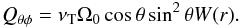 (4)The product νTΩ0 (Ω0 the characteristic angular velocity) is the scalar with the correct dimension, which reflects that only rotating turbulence possesses finite horizontal cross correlations. From Fig. 1 and with the solar value Ω0 = 2.6 × 10⁻⁶ s-1, we find W ≃ 0.3 /ν8 with ν8 = νT/ (108 m2/ s). Previous investigations with magnetic tracers have led to values for W that are higher by two orders of magnitude (Ward 1965; Schröter & Wöhl 1976; Gilman & Howard 1984; Balthasar et al. 1986), while the statistical analysis of coronal bright points yielded smaller numbers (Vrsnak et al. 2004). For solitary spots, Nesme-Ribes et al. (1993) find low negative correlations.
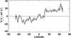 |
Fig. 1 Horizontal Reynolds stress ⟨ uθuφ ⟩ observed with the HMI on the SDO taken from Hathaway et. al. (2013).As it should, the quantity is antisymmetric with respect to the equator. Permission by D.H. Hathaway. |
The empirical results obviously indicate the invalidity of the simple Boussinesq relations (1) for rotating convection. The observed equatorial acceleration – if it is a deep-seated phenomenon – would always provide negative (positive) cross-correlation values for the northern (southern) hemisphere. Because this is not observed, it should be natural to replace the righthand expression (1) by 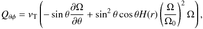 (5)where the second term on the righthand side is of cubic order in Ω. In this formulation the quantity H determines by its sign whether the angular momentum is transported equatorward (H> 0) or poleward (H< 0) by the Λ effect. Here, Ω0 is the basic rotation of the convection zone that will be fixed later on. The counterpart of (5) with respect to the radial transport of angular momentum is
 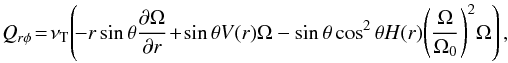 (6)where as in (2) also here a term V appears that is linear in Ω. All the nondiffusive terms in the expressions for the turbulent angular momentum transport can be written in the tensorial form Qij = ... + ΛijkΩk with the Λ effect tensor Λijk, which is even in the axial vector Ω by definition. This is why all terms in (5) and (6) are odd in Ω. A tensor of third rank even in Ω can only be constructed in turbulent fluids if the turbulence is anisotropic by itself and/or inhomogeneous as a consequence of the density stratification. Both conditions are fulfilled in stellar convection zones.
We have shown earlier by means of quasilinear turbulence theory that the function V is negative and exists mainly in the supergranulation layer, while H is positive and exists mainly in the bulk of the convection zone. Numerical simulations provide very similar results (Chan 2001; Käpylä et al. 2011; for more details see Rüdiger et al. 2013). We also know that the positive quantity H in (5) and (6) both contribute to the equatorial acceleration so that it is not trivial to find the sign of (4) as a function of depth.
Solving Eq. (3) with (5) and (6) leads for a simple model with uniform density, V and H, for stress-free boundaries (Qrφ = 0) and for thin shells to the estimates 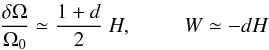 (7)for δΩ as the normalized equator-pole difference of Ω and the amplitude of W, both taken at the surface. Both observables do not depend on the viscosity value. Here d ≃ 0.3 is the normalized thickness of the convection zone. The negative sign of W means that the latitudinal shear at the surface always exceeds the value of H. The data of Fig. 1, however, concern the giant cell pattern that exists deep in the convection zone. The shear there is reduced by the lower boundary condition, which represents the action of the tachocline so that W becomes positive. The analytical relation for W at the bottom of the convection zone thus reads as W ≃ dH> 0. The observed positivity of cosθQθφ thus appears to be compatible with the existence of the solar tachocline, which rapidly reduces the equator-pole difference to zero (probably by Maxwell stress, see Rüdiger et al. 2013).
2. Mean-field models
We now solve the mean-field Eq. (3) in the northern hemisphere in the domain 0.6 ≤ x ≤ 1 (x is the fractional radius, x = r/R) with the natural boundary conditions ∂Ω /∂θ = 0 at the polar and the equatorial axes and the stress-free condition Qrφ = 0 at the surface. To model a fast tachocline-like transition at the bottom of the domain rigid-body rotation with Ω = Ω0 is prescribed there. The first-order term V is assumed to exist only in the outermost layers, while the third-order effect H exists down to the bottom of the convection zone at xin = 0.7. This simple but nonlinear model, which only ignores the transport of angular momentum by the meridional flow, yields the numerical results given in the Figs. 2–4, which demonstrate the characteristic behavior of the horizontal stress function W as the solution of the Reynolds Eq. (3).
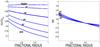 |
Fig. 2 Rotation law (left) and the horizontal Reynolds stress function W (right) for a mean-field model with V = 0 and H = 1 in the entire convection zone. The curves are marked with their latitudes. The density is assumed to be uniform. |
We start with uniform turbulence effects; i.e., V = 0 and H = 1 in the entire convection zone. It is then easy to see from (6) that the outer boundary condition requires ∂Ω /∂r = 0 at the equator and negative radial shear in higher latitudes. The immediate consequence is a uniform rotation beneath the equator and a very strong subrotation along the polar axis. The equator-pole difference of Ω is always positive, and it grows outward (Fig. 2). It is so strong at the surface that the W becomes negative there, while it takes high positive values in the bulk of the convection zone. Also the analytical estimates (7) are approximately fulfilled, although they are obtained with the highly simplified linear theory.
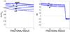 |
Fig. 3 Same as in Fig. 2 but with H = 1 only in the bulk of the convection zone (xin ≤ x ≤ 0.95) and V = −0.1 for x> 0.95. |
The rotation law in Fig. 2, however, fails to deliver the characteristic super-rotation of the solar equator at the bottom of the convection zone, which has been helioseismologically derived and which is the source of the “dynamo dilemma” (Parker 1987) because it prevents the reproduction of the butterfly diagram of the sunspot locations within the solar cycle. It is also known, however, that the simple model used for Fig. 2 does not correctly describe the radial profiles of the turbulent Λ terms. The linear-in-Ω term V mainly exists in the outer part of the convection zone, while the Ω3 term H only exists in the inner part of the convection zone (see Rüdiger et al. 2013). This has consequences for the outer boundary condition that now tends to produce negative gradients of Ω at all latitudes. The result for a model with V = −0.1 (for x> 0.95) and with H = 1 for xin ≤ x ≤ 0.95 is given in Fig. 3. Indeed, a weak equatorial superrotation is now indicated at the bottom of the convection zone. The latitudinal shear, however, is reduced so that the W after (4) becomes larger than in Fig. 2. It is again negative in the surface region where function H is small or even zero.
The equatorial acceleration is reduced in Fig. 3 in comparison to the results of the “uniform” model of Fig. 2. This is due to the absence of the function H in the outer layers. If the weight of these layers is reduced by a strong negative density gradient, then the surface rotation law recovers, and the observed value of the equator-pole difference of Ω appears again (Fig. 4). The used density profile is simply written as ρ ∝ exp(−x/G), which has been applied in the Reynolds Eq. (3) with G = 0.05 for the normalized density scale height.
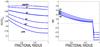 |
Fig. 4 Same as in Fig. 3 but with a density profile included, which decreases outward within the convection zone by more than six scale heights (G = 0.05). |
All the solutions of the nonlinear Eq. (3) for our model lead to the following results:
-
the equatorial acceleration is of the observed amount,
-
W< 0 at the surface and W> 0 in the subsurface layers,
-
W is positive if averaged over the radius.
3. Two solar models
We have also analyzed the horizontal Reynolds stress of the two basic mean-field models for the solar differential rotation established by Küker et al. (2011), including meridional circulation and anisotropic convective heat transport. The first one contains the full Reynolds stress tensor, while the other one works without the Λ effect (see Balbus et al. 2012). Both models are able to reproduce the surface rotation law (Fig. 5), but – as we shall see – they differ in the sign of the resulting meridional circulation and in the sign of the resulting horizontal Reynolds stress.
The convection zone model has been computed with the MESA stellar evolution code (Paxton et al. 2011). The Reynolds stresses were computed with a prescribed rotation period of 27 days, and a value of 5/3 for the mixing length parameter. This choice sets the mixing length equal to the density scale height. The viscosity coefficient νT of the models is of order 109 m2/s with a maximum of 2 × 10⁹ m2/s in a depth of x ≃ 0.8.
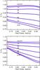 |
Fig. 5 Rotation laws Ω/Ω0 for the two models with (top) and without (bottom) Λ effect. The meridional circulation at the surface flows poleward (top) or equatorward (bottom). |
The model without the Λ effect results in an internal rotation pattern with disk-shaped iso-contours (at the equator region). The meridional flow is directed toward the equator at the surface and toward the poles at the bottom of the convection zone (“clockwise”). On the other hand, the model that is based on the Λ effect provides a meridional circulation cell with the opposite flow direction (“counterclockwise”).
Figure 6 gives the horizontal Reynolds stress Qθφ averaged over the radius in its dependence on the latitude. This quantity is antisymmetric with respect to the equator by definition and thus vanishes at the equator. If the Reynolds stress is purely viscous Qθφ is negative (positive) in the northern (southern) hemisphere, in contrast to the empirical findings given in Fig. 1. For the model with the full Reynolds stress the horizontal Λ effect exceeds the viscous part in the bulk of the convection zone, and the total Reynolds stress is positive (negative) in the northern (southern) hemisphere. As it must, the horizontal stress Qθφ vanishes both on the rotation axis and in the equatorial plane. It reaches its peak value at about 30° latitude. The amplitude of the horizontal cross correlation Qθφ is on the order of 100 m2/s2, which leads to | W | ≃ 0.14, so corresponding closely to the righthand estimate in (7) as from the quasilinear turbulence theory H ≃ 0.4 results. The value is in good agreement with the numerical results for the cubic Reynolds equation (see Fig. 4).
We have to note that the numerical value of the positive maximum of 100 m2/s2 exceeds the empirical results by a factor of five, which might be a consequence of the viscosity value used in the simulations that was too high or on details of the formulation of the lower boundary condition.
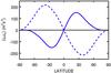 |
Fig. 6 Reynolds stress Qθφ from the simulations and averaged over the radius with Λ effect (solid) and without Λ effect (dashed). It always vanishes at the equator (see the empirical results of Fig. 1). |
4. Conclusions
It is hard to imagine that the mechanism of the solar dynamo could be understood without understanding the maintenance of the solar rotation law. It is thus highly relevant if one can show that the generation of the differential rotation of the solar
convection zone is based on the existence of nondiffusive Λ terms in the Reynolds stress in a similar sense to the solar dynamo being based on the existence of nondiffusive α terms in the induction equation. We argue that the Λ effect in rotating anisotropic turbulence is indeed needed to explain the current observation of positive (negative) horizontal cross correlation Qθφ in the northern (southern) hemisphere at the solar surface, which Hathaway et al. (2013) indicated as a result of the proper motions of giant cells. All analytical and numerical studies lead to positive functions H, which in the bulk of the convection zone are able to overcompensate for the diffusive term, which alone would lead to the signs that are not observed. The overcompensation, however, is not trivial. We have to mention in this respect that the H is a term of higher order in the Coriolis number Ω∗ = 2τcorrΩ so that due to the short lifetimes of the granulation and supergranulation H ≪ 1 in the outer part of the convection zone. The turbulent medium in the outer layer of the solar convection zone, therefore, behaves almost diffusively in the horizontal plane.
With a numerical model that ignores the meridional flow, we demonstrated that the quantity W is indeed negative in the surface layers. This, however, is only a surface effect. In subsurface layers the equator-pole difference of Ω is reduced, and the amplitude of the positive H grows. It is thus no surprise that in the deeper layers of the convection zone, the sign of W becomes positive. This general result does not depend on details of the eddy viscosity, of the density stratification, and/or of the influences of the meridional flow. Also, our most complex Λ effect model, which reproduces the internal solar rotation law and also the observed pattern of the meridional flow, shows the described behavior exactly. If the equatorial acceleration were exclusively due to a meridional flow (which in this case must flow equatorward along the surface), then the function W would be negative-definite on the northern hemisphere through the entire convection zone, but this is, however, not observed.
References
- Balbus, S. H., Latter, H., & Weiss, N. 2012, MNRAS, 420, 2457 [NASA ADS] [CrossRef] [Google Scholar]
- Balthasar, H., Vazquez, M., & Wöhl, H. 1986, A&A, 155, 87 [NASA ADS] [Google Scholar]
- Boussinesq, M. J. 1897, Théorie de l’écoulement tourbillonnant et tumultueux des liquides (Paris: Gauthier-Villars et fils) [Google Scholar]
- Chan, K. L. 2001, ApJ, 548, 1102 [NASA ADS] [CrossRef] [Google Scholar]
- Duvall, T. L. 1979, Sol. Phys., 63, 3 [NASA ADS] [CrossRef] [Google Scholar]
- Gilman, P. A., & Howard, R. 1984, Sol. Phys., 93, 171 [NASA ADS] [Google Scholar]
- Gizon, L., & Rempel, M. 2008, Sol. Phys., 251, 241 [NASA ADS] [CrossRef] [Google Scholar]
- Hathaway, D. H., Upton, L., & Colegrove, O. 2013, Science, 342, 1217 [NASA ADS] [CrossRef] [Google Scholar]
- Howard, R. 1979, ApJ, 228, L45 [NASA ADS] [CrossRef] [Google Scholar]
- Käpylä, P. J., Mantere, M. J., Guerrero, G., et al. 2011, A&A, 531, A162 [NASA ADS] [CrossRef] [EDP Sciences] [Google Scholar]
- Kippenhahn, R. 1963, ApJ, 137, 664 [NASA ADS] [CrossRef] [Google Scholar]
- Küker, M., Rüdiger, G., & Kitchatinov, L. L. 2011, A&A, 530, A48 [NASA ADS] [CrossRef] [EDP Sciences] [Google Scholar]
- Nesme-Ribes, E., Ferreira, E. N., & Vince, L. 1993, A&A, 276, 211 [NASA ADS] [Google Scholar]
- Parker, E. 1987, Sol. Phys., 110, 11 [Google Scholar]
- Paxton, B., Bildsten, L., Dotter, A., et al. 2011, ApJS, 192, 3 [Google Scholar]
- Reinhold, T., Reiners, A., & Basri, G. 2013, A&A, 560, A4 [NASA ADS] [CrossRef] [EDP Sciences] [Google Scholar]
- Rüdiger, G. 1989, Differential rotation and solar convection (Gordon & Breach Science Publishers) [Google Scholar]
- Rüdiger, G., Kitchatinov, L. L., & Hollerbach, R. 2013, Magnetic processes in astrophysics: theory, simulations, experiments (Weinheim: Wiley-VCH) [Google Scholar]
- Schad, A., Timmer, J., & Roth, M. 2012, Astron. Nachr., 333, 991 [NASA ADS] [CrossRef] [Google Scholar]
- Schröter, E. H., & Wöhl, H. 1976, Sol. Phys., 49, 19 [NASA ADS] [CrossRef] [Google Scholar]
- Taylor, G. I. 1915, Phil. Trans. Roy. Soc. Lond., A215, 1 [Google Scholar]
- Vrsnak, B., Brajsa, R., Wöhl, H., et al. 2003, A&A, 404, 1117 [NASA ADS] [CrossRef] [EDP Sciences] [Google Scholar]
- Ward, F. 1965, ApJ, 141, 534 [NASA ADS] [CrossRef] [Google Scholar]
All Figures
|
Fig. 1 Horizontal Reynolds stress ⟨ uθuφ ⟩ observed with the HMI on the SDO taken from Hathaway et. al. (2013).As it should, the quantity is antisymmetric with respect to the equator. Permission by D.H. Hathaway. |
| In the text | |
|
Fig. 2 Rotation law (left) and the horizontal Reynolds stress function W (right) for a mean-field model with V = 0 and H = 1 in the entire convection zone. The curves are marked with their latitudes. The density is assumed to be uniform. |
| In the text | |
|
Fig. 3 Same as in Fig. 2 but with H = 1 only in the bulk of the convection zone (xin ≤ x ≤ 0.95) and V = −0.1 for x> 0.95. |
| In the text | |
|
Fig. 4 Same as in Fig. 3 but with a density profile included, which decreases outward within the convection zone by more than six scale heights (G = 0.05). |
| In the text | |
|
Fig. 5 Rotation laws Ω/Ω0 for the two models with (top) and without (bottom) Λ effect. The meridional circulation at the surface flows poleward (top) or equatorward (bottom). |
| In the text | |
|
Fig. 6 Reynolds stress Qθφ from the simulations and averaged over the radius with Λ effect (solid) and without Λ effect (dashed). It always vanishes at the equator (see the empirical results of Fig. 1). |
| In the text | |
Current usage metrics show cumulative count of Article Views (full-text article views including HTML views, PDF and ePub downloads, according to the available data) and Abstracts Views on Vision4Press platform.
Data correspond to usage on the plateform after 2015. The current usage metrics is available 48-96 hours after online publication and is updated daily on week days.
Initial download of the metrics may take a while.