| Issue |
A&A
Volume 572, December 2014
|
|
|---|---|---|
| Article Number | A14 | |
| Number of page(s) | 6 | |
| Section | Astronomical instrumentation | |
| DOI | https://doi.org/10.1051/0004-6361/201424476 | |
| Published online | 19 November 2014 | |
Multiwavelength active-optics Shack-Hartmann sensor for monitoring seeing and turbulence outer scale
Laboratoire Lagrange, UMR 7293, Université de Nice Sophia-Antipolis, CNRS, Observatoire de la Côte d’Azur, Bd. de l’Observatoire, 06304 Nice, France
e-mail: This email address is being protected from spambots. You need JavaScript enabled to view it.
Received: 26 June 2014
Accepted: 21 August 2014
Abstract
Context. Real-time seeing and outer-scale estimation at the location of the focus of a telescope is fundamental for predicting the adaptive-optics system’s dimensioning and performance, as well as for the operational aspects of instruments.
Aims. This study attempts to take advantage of multiwavelength long-exposure images to instantaneously and simultaneously derive the turbulence outer scale and seeing from the full width at half maximum (FWHM) of seeing-limited images taken at the focus of a telescope. These atmospheric parameters are commonly measured in most observatories by different methods located away from the telescope platform, thus differing from the effective estimates at the focus of a telescope, mainly because of differences in pointing orientation, height above the ground, or local seeing bias (dome contribution).
Methods. Long-exposure images can either be provided directly by any multiwavelength scientific imager or spectrograph or, alternatively from a modified active-optics Shack-Hartmann sensor (AOSH). From measuring the AOSH sensor spot point spread function FWHMs simultaneously at different wavelengths, one can estimate the instantaneous outer scale in addition to seeing.
Results. Multiwavelength long-exposure images provide access to accurate estimates of r0 and L0 by adequate means as long as precise FWHMs can be obtained. Although AOSH sensors are specified to measure not spot sizes but slopes, real-time r0, and L0 measurements from spot FWHMs can be obtained at the critical location where they are needed with major advantages over scientific instrument images: insensitivity to the telescope field stabilization, and continuous availability.
Conclusions. Assuming an alternative optical design that allows simultaneous multiwavelength images, the AOSH sensor benefits from all the advantages of real-time seeing and outer scale monitoring. With the substantial interest in the design of extremely large telescopes, such a system could be of considerable importance.
Key words: atmospheric effects / instrumentation: adaptive optics / site testing / methods: numerical
© ESO, 2014
1. Introduction
Atmospheric seeing is commonly measured by the differential image motion monitor (DIMM, Sarazin & Roddier 1990) in most observatories, or by means of alternative seeing monitors, e.g., Generalized Seeing Monitor (GSM, Ziad et al. 2000), Multi-Aperture Scintillation Sensor (MASS, Kornilov & Tokovinin 2001). Since it is localized away from the telescope platform, the DIMM delivers a seeing estimate that can differ significantly from the effective seeing as seen at a telescope focus because of pointing orientation and/or differences in height above the ground, or local seeing bias (dome contribution). The effect of the two last will substantially expand in the next generation of telescopes: the extremely large telescopes (ELTs).
Evaluating of the seeing is paramount for selecting astronomical sites and/or following their temporal evolution. Likewise, its estimation is fundamental for dimensioning adaptive optics (AO) systems and their performance predications. In this context, the outer scale of the turbulence, related as the distance over which the spatial power spectral density of phase distortions deviates from the pure 5/3 power law at low frequencies (associated with the Kolmogorov-Obukhov turbulence model), it plays a significant role in AO systems. In particular, the power in the lowest Zernike aberration modes (e.g., tip and tilt) is strongly affected, and the knowledge of reliable estimate of L0 is of considerable importance in the future area of the ELTs. As a consequence, knowledge of both seeing and L0 virtually drive instrument designs or operational aspects at a telescope, and more emphasis is put on developing accurate real-time seeing and outer scale monitors at the focus of a telescope.
For this purpose, various flavors of images can be used at the critical location of the telescope focus: (1) scientific instrument images; (2) guide-probe images; and (3) active-optics Shack-Hartmann images. At the VLT (the Very Large Telescope at the ESO Paranal observatory), focal planes are equipped with an arm used for acquiring of a natural guide star. The light from this star is then split between a guide probe for an accurate tracking of the sky, and a Shack-Hartmann wavefront sensor used by the active-optics to control the shape of the primary mirror. In this context, estimating the seeing from the full width at half maximum (FWHM) of a PSF strongly relies on the exposure time that must be long enough so that the turbulence has been averaged (ensuring that all representations of the wavefront spatial scales have passed through the pupil). This depends on telescope diameter and turbulence velocity, though it is commonly admitted that 30 s is the proper average of the turbulence and that significant FWHM biases would otherwise be introduced. Since the guide probe has exposure times that are no longer than 50 millisec, it cannot be used as a seeing/outer scale monitor. The active-optics Shack-Hartmann (AOSH) sensor includes all the advantage of real-time monitoring of these turbulence parameters. While most of the instruments are affected by observational bias (unavailability for a wide range of seeing conditions) and are affected by the telescope field stabilization, AOSH delivers continuous real-time images of long-exposure-spot PSFs (typically 45 s) at the same location as do scientific instruments. AOSH images simultaneously provide various data: slopes, intensities, and spot sizes. When short exposures are used, the information provided by both slopes and intensities (i.e., scintillation) can be used to retrieve Cn2 profile using correlations of these data from two separated stars (Robert et al. 2011; Voyez et al. 2013). When long exposures are used, it is feasible to retrieve the atmospheric seeing in the line of sight from the spot sizes in the sub-apertures, with the advantage of being insensitive to the telescope field stabilization (Martinez et al. 2012). While in most observatories the trend is to compare instrument image quality to DIMM or telescope guide camera FWHM measurements of the seeing in order to estimate L0 (e.g., Floyd et al. 2010), in this paper, we propose to use the AOSH sensor system of the telescope as a turbulence monitor to provide accurate seeing estimation directly at the telescope focus, with the additional measurement of the instantaneous turbulence outer scale L0 through multiwavelength exposures. For this purpose, an alternative optical configuration of the AOSH system is proposed, and the accuracy of seeing and L0 estimation is analyzed through extensive simulations.
2. Analytical treatment
2.1. Long-exposure seeing-limited PSF
The theoretical expression of a long-exposure seeing-limited PSF can be described through the Fourier transform (FT) of its optical transfer function (OTF). The OTF is obtained by multiplying the telescope OTF, denoted T0(f), by the atmospheric OTF: ![Mathematical equation: \begin{equation} T_{\rm a} (\vec{f}) = \exp \left[-0.5 D_{\phi}(\lambda \vec{f})\right], \label{eq:Tf} \end{equation}](/articles/aa/full_html/2014/12/aa24476-14/aa24476-14-eq6.png) (1)where f is the angular spatial frequency, λ the imaging wavelength, and Dφ(r) the phase structure function (Goodman 1985; Roddier 1981). Equation (1) is appropriate to any turbulence spectrum and any telescope diameter.
(1)where f is the angular spatial frequency, λ the imaging wavelength, and Dφ(r) the phase structure function (Goodman 1985; Roddier 1981). Equation (1) is appropriate to any turbulence spectrum and any telescope diameter.
The standard theory based on the Kolmogorov-Obukhov model (Tatarskii 1961) provides the analytic expression for the phase structure function and is expressed by  (2)This theory describes the shape of the atmospheric long-exposure PSF by a single parameter, the Fried’s coherence radius r0 (Fried 1966), and the long-exposure OTF is expressed as
 ![Mathematical equation: \begin{eqnarray} T(\vec{f}) = T_{0} (\vec{f}) \times \exp\left[-3.44 (\lambda \vec{f}/r_{0})^{5/3}\right]. \label{A1} \end{eqnarray}](/articles/aa/full_html/2014/12/aa24476-14/aa24476-14-eq11.png) (3)In the case of a large ideal telescope with diameter D ≫ r0, the diffraction term T0 can be neglected.
(3)In the case of a large ideal telescope with diameter D ≫ r0, the diffraction term T0 can be neglected.
However, it is commonly accepted that Eq. (3) assumes non-realistic behavior of the low-frequency content of the turbulence model phase spectrum, and it is firmly established that the phase spectrum deviates from the power law at low frequencies (Ziad et al. 2000; Tokovinin et al. 2007). This behavior is described in a first order by an additional parameter, the outer scale L0. This additional parameter is introduced by the Von Kàrmàn (vK) turbulence model (e.g., Tatarskii 1961; Ziad et al. 2000), and the mathematical definition of L0 is given by  (4)where Wφ(f) represents the phase distortions. In this context, the Kolmogorov-Obukhov model corresponds to L0 = ∞, and in the vK model r0 describes the high-frequency asymptotic behavior of the spectrum. Physically, L0 is related to the largest size of perturbations, and corresponds to a reduction in the low-frequency content of the phase perturbation spectrum. Nonetheless, the vK is not a verified model. It is established that the phase spectrum does deviate from a power law, and existing experimental data on L0 are interpreted in this sense. The value of L0 does not depend on wavelength, and typical values are on the order of 20 m with a scatter that can be as large as a few hundred meters (Ziad et al. 2000; Tokovinin et al. 2007).
In the vK model, the expression for the phase structure function (Dφ) with finite outer scale L0 can be found in Tatarskii (1961) or Tokovinin (2002): ![Mathematical equation: \begin{eqnarray} D_{\phi}(\vec{ r})& =& \frac{\Gamma(11/6)}{2^{11/6} \pi^{8/3}} \left[\frac{24}{5} \Gamma \left(\frac{6}{5} \right) \right]^{5/6} \left( \frac{r_{0}}{L_0} \right)^{-5/3} \nonumber\\ &&\times~ \left[2^{-1/6} \Gamma \left( \frac{5}{6} \right) - \left( \frac{2 \pi r}{L_0} \right)^{5/6} K_{5/6} \left( \frac{2 \pi r}{L_0} \right) \right], \label{eq:SF} \end{eqnarray}](/articles/aa/full_html/2014/12/aa24476-14/aa24476-14-eq18.png) (5)where K5/6(x) is the modified Bessel function of the third kind, and Γ(x) is the gamma function. Putting the vK phase structure function into Eq. (3), we obtain the atmospheric long-exposure OTF expression, which now depends on both ε0 and L0. While it is understood that for finite L0, Eq. (3) does not go to zero at high spatial frequencies (the FT of Ta(f) formally does not exist), but when r0 ≪ L0, it can be neglected.
(5)where K5/6(x) is the modified Bessel function of the third kind, and Γ(x) is the gamma function. Putting the vK phase structure function into Eq. (3), we obtain the atmospheric long-exposure OTF expression, which now depends on both ε0 and L0. While it is understood that for finite L0, Eq. (3) does not go to zero at high spatial frequencies (the FT of Ta(f) formally does not exist), but when r0 ≪ L0, it can be neglected.
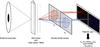 |
Fig. 1 Principle of the two-wavelength active-optics Shack-Hartmann sensor. |
2.2. Seeing, outer scale, and FWHM
The Kolmogorov-Obukhov model predicts dependence of the PSF FWHM ε0 on wavelength λ and r0:  (6)However, because the outer scale of turbulence L0 describes the low-frequency behavior of the turbulence model phase spectrum, it plays a significant role in the image FWHM at the focus of a telescope. The image FWHM is different, and the difference can be as much as 30% to 40% in the near-infrared, from the atmospheric seeing that can be measured by dedicated seeing monitors, such as the DIMM (Sarazin & Roddier 1990).
The seeing measured by the DIMM is sensitive to small-scale wavefront distortions, and thus provides estimates that are almost independent of the outer scale of the turbulence L0. The dependence of atmospheric long-exposure resolution on L0 is efficiently predicted by a simple approximate formula (Eq. (7)) introduced by Tokovinin (2002) and confirmed by means of extensive simulations (Martinez et al. 2010b,a), where it is emphasized that the effect of finite L0 is independent of the telescope diameter. The validity of Eq. (7) has been established in an L0/r0> 20 and L0/D ≤ 500 domain (Martinez et al. 2010b), where D is the telescope diameter (the treatment of the diffraction failed for small telescope diameters, D< 1m). As a consequence, long-exposure seeing-limited PSF FWHM (εvK) are directly related to ε0 (or alternatively r0) and L0 as 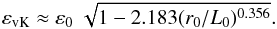 (7)Deducing the atmospheric seeing ε0 from the FWHM of a long-exposure, seeing-limited PSF at the focus of a telescope requires the correction implied by Eq. (7) with either the knowledge of L0 (simultaneously measured by any means) or the correction by an a priori L0 value selected from a long-term monitoring of the observational site (usually the median value is retained, e.g., L0 = 22 m at Paranal), prior to airmass and wavelength correction. It is trivial to see that these two parameters (ε0, or alternatively r0, and L0) cannot be simultaneously deduced from a single long-exposure seeing-limited PSF FWHM (i.e., a single wavelength exposure provide a unique FWHM estimate, while two parameters are undetermined).
2.3. Multiwavelength FWHMs
A straightforward way to solve the indetermination is to consider a multiwavelength FWHM measurement. In the following, and for the sake of generality, n measurements will be assumed, while only two are required to resolve the current problem. In the context of n-wavelength, long-exposure seeing-limited PSF FWHM measurements, Eq. (7) can be formalized as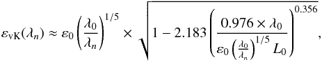 (8)where λn is the wavelength of the exposure considered, λ0 is the wavelength of 500 nm, adopted as standard for seeing computation, and r0 has been replaced by ε0 using Eq. (6). Equation (8) now provides n different εvK estimations, for two unknown parameters (ε0 and L0) and can be simplified as:
 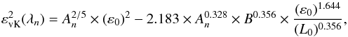 (9)where An = λ0/λn and B = 0.976 × λ0. Finally, a simple expression can be obtained:
  (10)where U and V are equal to
  and
and  , respectively. A numerical resolution of the system solving for U and V where n = 2 can be trivially achieved with a standard singular value decomposition method.
3. Numerical simulations
The schematic representation of the modified AOSH sensor considered to provide two-wavelength images is presented in Fig. 1. It is based on the standard principle of the AOSH except that at a focal plane downstream of the Shack-Hartmann lenslet array, the light from the telescope pupil is focused at the tip of a roof prism, which splits the light into two parts. These two separated beams propagate through different spectral filters. Finally, the incoming light of these two optical arms is dissected by individual lenslet arrays, which then focus the light onto the detector array. The lenslet array creates a number of separated focal spots of light on the detector. As part of the telescope active-optics system, such a system has the advantage of delivering continuously spot images (unaffected by observational bias in contrast to scientific instruments). Retrieving atmospheric seeing ε0 (at 500 nm) from the FWHM of a unique (single-wavelength) long-exposure seeing-limited PSF image requires the correction implied by Eq. (7) (prior to airmass and wavelength correction). I remind the reader that it even concerns the case of small-size (d) AOSH subapertures, where L0≫d, and the examination of the L0 influence was also treated (Martinez et al. 2012). Accurate seeing estimation by means of a dedicated algorithm and upon adequate calibration is demonstrated in Martinez et al. (2012). The following sections explain the details of the simulations involved in the study.
3.1. Atmospheric turbulence
The atmospheric turbulence is simulated with hundreds to thousands of uncorrelated phase screens of dimension 4096 × 4096 pixels (i.e., 60 m width) to allow long-exposure images (>30 s) upon atmospheric conditions. The principle of the generation of a phase screen is based on the standard Fourier approach, where randomized white noise maps are colored in the Fourier space by the turbulence power-spectral-density (PSD) function, and the inverse Fourier transform of an outcome corresponds to a phase screen realization. The validity of the atmospheric turbulence statistic has been verified on the simulated phase screens: the value of the outer scale (L0), Fried parameter (r0), and seeing of the phase screens has been confirmed by decomposition on the Zernike polynomials and variance measurements over the uncorrelated phase screens. In addition, the validity of the long-exposure AOSH image has been verified. In Fig. 2, we show an example of the simulated AOSH image (based on the ESO VLT AOSH configuration).
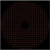 |
Fig. 2 Simulated AOSH image based on the VLT AOSH geometry. |
3.2. Shack-Hartmann model
Simulations are based on a diffractive Shack-Hartmann model that reproduces the VLT AOSH geometry, mimicking the 24 subapertures across the pupil diameter of the VLT active-optics, with 22 pixels per subaperture, and 0.305″ pixel scale (d = D/ 24 = 0.338 m). The validity of the AOSH model has been verified through several aspects, such as the plate scale, spot sizes, slope measurements, and phase reconstruction. The AOSH paradigm is presented in Fig. 2. Background estimation is performed on a corner of the image without spots, and hot pixels are set to the background. The cleanest and unvignetted spots are selected in each frame for the analysis. These extracted spots are oversampled by a factor two, recentered and averaged. The averaging reduces the influence of potential local CCD defects, though these are not included in the simulation. In practice, the averaged spot is based on hundreds of selected spots. More than 400 spots over 526 available are usually selected for the analysis. The multiwavelength AOSH simulator provides four images at four different wavelengths (0.5, 0.55, 0.6, and 0.65 μm), while only two are used and analyzed (0.5 and 0.55 μm). The choice of the wavelength values used in simulation is arbitrary, and its optimization is beyond the scope of the present study. While an optimal combination can certainly be found by considering system and telescope operational aspects (e.g., photon noise, bandpasses, subsystem characteristics, and pertaining constraints, etc.), once the wavelengths are known and corresponding FWHMs correctly estimated, seeing and outer scale are accurately retrieved regardless of the wavelength combination selected.
3.3. Extraction of the FWHM
The algorithm used to extract the FWHM from the AOSH sensor spots has been proposed by Tokovinin et al. (2007) and extensively analyzed in Martinez et al. (2012). It is based on the long-exposure spot PSF profile defined in Eq. (3). The modulus of the long-exposure optical transfer function of the averaged spot is calculated and normalized. It is then divided by the square subaperture diffraction-limited transfer function T0(f): ![Mathematical equation: \begin{equation} T_{0}(\vec{f}) = (1-[\lambda \vec{f}_x/\vec{d}]) \times (1 - [\lambda \vec{f}_y/\vec{d}]). \label{diff1} \end{equation}](/articles/aa/full_html/2014/12/aa24476-14/aa24476-14-eq56.png) (11)In the case of a large ideal telescope with diameter D ≫ r0, the diffraction term T0 of Eq. (3) can be neglected, while in the case of AOSH subapertures of size d, it cannot (d ≈ r0). At this stage the cut of the T(f) along each axis can be extracted and fitted to the exponential part of Eq. (3) to derive a single parameter r0, or equivalently, Fourier-transformed to derive the FWHM of the resulting spot PSF profile using a two-dimensional elliptical Gaussian fit (a Moffat or a 10th-order polynomial fit can be selected instead). The orientation of the long and small axes of T(f) is found by fitting it with a two-dimensional elliptical Gaussian.
(11)In the case of a large ideal telescope with diameter D ≫ r0, the diffraction term T0 of Eq. (3) can be neglected, while in the case of AOSH subapertures of size d, it cannot (d ≈ r0). At this stage the cut of the T(f) along each axis can be extracted and fitted to the exponential part of Eq. (3) to derive a single parameter r0, or equivalently, Fourier-transformed to derive the FWHM of the resulting spot PSF profile using a two-dimensional elliptical Gaussian fit (a Moffat or a 10th-order polynomial fit can be selected instead). The orientation of the long and small axes of T(f) is found by fitting it with a two-dimensional elliptical Gaussian.
3.4. Solving ε0 and L0 from FWHMs
Various methods for solving a set of n linear equations in n unknowns are available, such as least squares fitting or LU (lower/upper) decomposition. In practice, the standard LU decomposition has been successfully used to solve our square system of linear equations. The programming language is IDL using the linear algebra library package LAPACK.
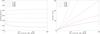 |
Fig. 3 Impact of a differential error in the estimation of the FWHM measured at 0.5 and 0.55 μm with the two-wavelength AOSH sensor on the seeing estimate (left) and turbulence outer scale estimate (right). The dashed and black lines represent the case where no error is applied. |
4. Results and discussion
4.1. General results
The series of tests conducted to determine the ability of a multiwavelength AOSH sensor to sort out seeing and turbulence outer scale values are twofold: (1) under a specific simulated seeing condition (0.83″, ESO Paranal observatory median seeing value as measured by the DIMM at 6 meters height from the ground), several turbulence outer scale conditions are simulated, and simulated/estimated parameters can be compared; (2) for a particular generated turbulence outer scale value, several seeing conditions (ranging from 0.6 to 1.8″) were simulated. Estimated and simulated parameters were then again compared. This latest test was repeated for two outer scale values (22 and 30 m, where 22 m is the Paranal observatory median value).
At this stage, two aspects should be pointed out, both related to the sampling issue. (1) Higher outer scale values than 30 m cannot in principle be considered because the simulated atmospheric phase screens are physically limited to 60 m width. It was indeed observed that above roughly 40 m phase screen sides, the outer scale estimation failed to be accurate. (2) There is a catch in matching the simulated AOSH sensor to the one of the VLT: the pixel scale is crude (0.305″). This has been pointed out in Martinez et al. (2012): seeing estimates under 0.6″ failed to be accurate, while probably seeing values above 0.6″ are still affected to a certain extent by the effect of undersampling. This point will be discussed further in the Sect. 4.3, where the AOSH geometry is modified (by simulating AOSH sensor with various subapertures configurations but identical telescope pupil footprint in pixel, in order to increase or decrease the pixel sampling, e.g., 6 × 6, 9 × 9, 18 × 18, 24 × 24, and 48 × 48 subapertures).
Table 1 summarizes the results obtained under various turbulence outer scale values coupled with 0.83″ seeing conditions. Both seeing and outer scale values are estimated well from the AOSH images. The seeing is accurate at a 10-2 level, while the outer scale is fairly estimated with a maximum error margin of two meters. Table 2 presents the results under various seeing conditions with two outer scale values (22 and 30 m). For the 22 m outer scale set of data, the mean value of the estimated outer scale is 24.5 m with a standard deviation of 7.9 m, while for the 30 m outer scale set of data, the mean value is 28.7 m with a standard deviation of 5.7 m. In all cases, the seeing estimate is fairly good, accurate at a few 10-2 level. In addition, from Table 2 it is observable that the better the seeing, the worse the outer scale estimates. Increasing the seeing estimate accuracy is therefore fundamental for increasing the accuracy of the outer scale estimation. This is likely due to the outcome of the pixel scale problem, which directly affects the accuracy of the FWHM estimates. This point is addressed in the next section.
Seeing and L0 estimations for various L0 values under 0.83″ seeing conditions.
Seeing and L0 estimations for various seeing conditions.
Effect of the subaperture sampling on the measured FWHM.
4.2. Sensitivity analysis
Precise FWHM estimation from the spot images is mandatory to deliver accurate seeing and outer scale monitoring with the AOSH sensor. This is a major concern for the outer scale estimate more than for the seeing itself. This is observable in Fig. 3 where the impact of a differential error on the calculation of the two FWHMs is appraised. The evaluation of the FWHMs from spot images is not perfect, and some errors are committed during the calculation for various reasons: internal system aberrations, spot under or poor sampling, insufficient signal-to-noise, etc. However, it is likely that this unavoidable amount of error involved in this estimation will apply almost similarly for both wavelength measurements, and the impact on the seeing and outer scale estimates will therefore be small because the errors committed at the two wavelengths will roughly compensate for each other. As a result, only the differential error between the two wavelengths matters. This is precisely what is addressed in the following. Using Eqs. (7) and (10) makes it straightforward to compute the seeing and outer scale values knowing the theoretically corresponding FWHMs at 0.5 and 0.55 μm. The test was done for a 0.83″ seeing and various outer scale values by introducing a small error in the theoretical FWHM at 0.5 μm. The FWHM computed at 0.55 μm is left unaffected. The impact of this error on the resolution of the multiwavelength system (Eq. (10)) is then plotted in Fig. 3, where the impact on the seeing estimate (left) and outer scale estimate (right) are shown.
The impact is not significant for the seeing evaluation, but is for the outer scale. The seeing estimation is mainly affected for low outer scale values (<30 m) and the evolution almost stabilizes for high outer scale values (>100 m). The impact on the outer scale estimate behaves in opposite way. Low outer scale values are less sensitive to FWHM error than high ones. The departure from the expected value (a dashed black line, i.e., with no error) can be significant, and degrades further with the outer scale. While a reasonable differential error in the estimation of the two-wavelength FWHMs has little impact on the seeing estimation, the impact on the outer scale can be considerable. This raises the importance of either developing a dedicated and accurate algorithm to precisely evaluate FWHMs from AOSH sensor spots upon adequate calibration (Martinez et al. 2012) or developing an optimized optical design for the multiwavelength AOSH sensor struggled for high sampling of the spots on the detector.
4.3. Subaperture sampling
The sampling effect is analyzed by modifying the AOSH pattern. While the footprint in pixel of the lenslet array is left unmodified, the number of subapertures is varying to allow changing the number of pixels per subaperture. Various configurations are tested (from 6 × 6 to 48 × 48 subapertures), where the FWHMs can be compared to predictions by Eq. (7). The results presented in Table 3 are unambiguous: the higher the sampling, the more accurate the FWHM. Subaperture sampling can only be calibrated but to a certain extent, and the effect is not linear with the seeing. Poor subaperture sampling calibration will not be as efficient as for a mild situation. This is a key aspect in the AOSH parameter space to consider when designing a multiwavelength AOSH system.
5. Conclusion
Although AOSH sensors are specified to measure slopes not spot sizes, the principle of the multiwavelength AOSH sensor was demonstrated and emerges as a potential efficient system for real-time seeing and instantaneous monitoring of turbulence outer scale. It offers direct access to important turbulence parameters at the precise location where we need them (at the focus of the telescope). Multiwavelength AOSH delivers long-exposure PSFs without being affected by any observational bias in contrast to scientific instruments and with being insensitive to the telescope field stabilization.
In addition, the AOSH design as proposed has the advantage of permitting calibration of the internal aberrations present in the system/telescope downstream of the roof prism. It precludes
their contribution to the spot FWHMs. The present study shows that accurate estimates of seeing and turbulence outer scale can reasonably be achieved with current systems, while the reliability of such a system can easily be increased with a better sampling of the spot PSFs. Assuming an alternative optical design that allows simultaneous multiwavelength images, the AOSH sensor is a good candidate for monitoring seeing and outer scale, especially in the vicinity of the ELT area.
References
- Floyd, D. J. E., Thomas-Osip, J., & Prieto, G. 2010, PASP, 122, 731 [NASA ADS] [CrossRef] [Google Scholar]
- Fried, D. L. 1966, J. Opt. Soc. Am., 56, 1372 [NASA ADS] [CrossRef] [Google Scholar]
- Goodman, J. W. 1985, Statistical Optics (New York: John Wiley and Sons) [Google Scholar]
- Kornilov, V. G., & Tokovinin, A. A. 2001, Astro. Rep., 45, 395 [NASA ADS] [CrossRef] [Google Scholar]
- Martinez, P., Kolb, J., Sarazin, M., & Tokovinin, A. 2010a, The Messenger, 141, 5 [NASA ADS] [Google Scholar]
- Martinez, P., Kolb, J., Tokovinin, A., & Sarazin, M. 2010b, A&A, 516, A90 [NASA ADS] [CrossRef] [EDP Sciences] [Google Scholar]
- Martinez, P., Kolb, J., Sarazin, M., & Navarrete, J. 2012, MNRAS, 421, 3019 [NASA ADS] [CrossRef] [Google Scholar]
- Robert, C., Voyez, J., Védrenne, N., & Mugnier, L. 2011 [arXiv:1101.3924] [Google Scholar]
- Roddier, F. 1981, Prog. in Optics (Amsterdam: North-Holland Publishing Co), 19, 281 [Google Scholar]
- Sarazin, M., & Roddier, F. 1990, A&A, 227, 294 [NASA ADS] [Google Scholar]
- Tatarskii, V. I. 1961, Wave Propagation in Turbulent Medium (McGraw-Hill) [Google Scholar]
- Tokovinin, A. 2002, PASP, 114, 1156 [NASA ADS] [CrossRef] [Google Scholar]
- Tokovinin, A., Sarazin, M., & Smette, A. 2007, MNRAS, 378, 701 [NASA ADS] [CrossRef] [Google Scholar]
- Voyez, J., Robert, C., Conan, J.-M., et al. 2013, in Proc. of the 3d AO4ELT Conf., eds. S. Esposito, & L. Fini, Id 68 [Google Scholar]
- Ziad, A., Conan, R., Tokovinin, A., Martin, F., & Borgnino, J. 2000, Appl. Opt., 39, 5415 [NASA ADS] [CrossRef] [PubMed] [Google Scholar]
All Tables
All Figures
|
Fig. 1 Principle of the two-wavelength active-optics Shack-Hartmann sensor. |
| In the text | |
|
Fig. 2 Simulated AOSH image based on the VLT AOSH geometry. |
| In the text | |
|
Fig. 3 Impact of a differential error in the estimation of the FWHM measured at 0.5 and 0.55 μm with the two-wavelength AOSH sensor on the seeing estimate (left) and turbulence outer scale estimate (right). The dashed and black lines represent the case where no error is applied. |
| In the text | |
Current usage metrics show cumulative count of Article Views (full-text article views including HTML views, PDF and ePub downloads, according to the available data) and Abstracts Views on Vision4Press platform.
Data correspond to usage on the plateform after 2015. The current usage metrics is available 48-96 hours after online publication and is updated daily on week days.
Initial download of the metrics may take a while.