| Issue |
A&A
Volume 572, December 2014
|
|
|---|---|---|
| Article Number | A97 | |
| Number of page(s) | 4 | |
| Section | Numerical methods and codes | |
| DOI | https://doi.org/10.1051/0004-6361/201424180 | |
| Published online | 03 December 2014 | |
Constraining duty cycles through a Bayesian technique⋆
1 INAF, Istituto di Astrofisica Spaziale e Fisica Cosmica – Palermo, via U. La Malfa 153, 90146 Palermo, Italy
e-mail: This email address is being protected from spambots. You need JavaScript enabled to view it.
2 Dipartimento di Fisica e Scienze della Terra, Università di Ferrara, via Saragat 1, 44122 Ferrara, Italy
3 Institut für Astronomie und Astrophysik, Eberhard Karls Universität, Sand 1, 72076 Tübingen, Germany
4 ISDC Data Center for Astrophysics, Université de Genève, 16 chemin d’Écogia, 1290 Versoix, Switzerland
Received: 11 May 2014
Accepted: 15 October 2014
Abstract
The duty cycle (DC) of astrophysical sources is generally defined as the fraction of time during which the sources are active. It is used to both characterize their central engine and to plan further observing campaigns to study them. However, DCs are generally not provided with statistical uncertainties, since the standard approach is to perform Monte Carlo bootstrap simulations to evaluate them, which can be quite time consuming for a large sample of sources. As an alternative, considerably less time-consuming approach, we derived the theoretical expectation value for the DC and its error for sources whose state is one of two possible, mutually exclusive states, inactive (off) or flaring (on), as based on a finite set of independent observational data points. Following a Bayesian approach, we derived the analytical expression for the posterior, the conjugated distribution adopted as prior, and the expectation value and variance. We applied our method to the specific case of the inactivity duty cycle (IDC) for supergiant fast X-ray transients, a subclass of flaring high mass X-ray binaries characterized by large dynamical ranges. We also studied IDC as a function of the number of observations in the sample. Finally, we compare the results with the theoretical expectations. We found excellent agreement with our findings based on the standard bootstrap method. Our Bayesian treatment can be applied to all sets of independent observations of two-state sources, such as active galactic nuclei, X-ray binaries, etc. In addition to being far less time consuming than bootstrap methods, the additional strength of this approach becomes obvious when considering a well-populated class of sources (Nsrc ≥ 50) for which the prior can be fully characterized by fitting the distribution of the observed DCs for all sources in the class, so that, through the prior, one can further constrain the DC of a new source by exploiting the information acquired on the DC distribution derived from the other sources.
Key words: methods: statistical / methods: numerical / methods: observational / X-rays: binaries
R-Language, IDL, and C-language programs are only available at the CDS via anonymous ftp to cdsarc.u-strasbg.fr (130.79.128.5) or via http://cdsarc.u-strasbg.fr/viz-bin/qcat?J/A+A/572/A97
© ESO, 2014
1. Introduction
In astrophysics it is often crucial to determine the duty cycle (DC) of a source, or a class of sources, in order to understand both their central engines and to plan additional observing campaigns aiming at best studying them. Generally, the DC is defined as the fraction of time, usually expressed in percentages, during which the source is active, or  (1)where Tactive is the time spent above some instrumental threshold or some scientifically interesting flux value, and TTot is the total exposure. In the case of periodic sources, such as classical X−ray binaries, Tactive is generally the time during which an n-σ detection is achieved (n being 3 or 5, depending on the detection method), and TTot is the orbital period Porb or the spin period Pspin (e.g. Henry & Paik 1969; Fragos et al. 2009; Knevitt et al. 2014).
For active galactic nuclei (AGNs), the DC is often defined as the fraction of time a source spends in a flaring state, that is, at n times the average flux,  , with n being a small number, depending on the purpose of the study (e.g. Jorstad et al. 2001; Vercellone et al. 2004; Ackermann et al. 2011). For example, in Vercellone et al. (2004) the DC is defined as
  where T is the time spent in a low flux level (off state) and τ is the time spent in a high flux level (on state), defined by
  , where Ci = 1 if
  and Ci = 0 otherwise.
Alternatively, when a source shows a very large dynamical range (a few orders of magnitude), more can be inferred about its nature by considering the inactivity duty cycle (IDC, Romano et al. 2009) defined as the time a source remains undetected down to a certain flux limit Flim, ![Mathematical equation: \begin{equation} \label{sfxtsims:eq:IDC} {\rm IDC}= \Delta T_{\Sigma}/[\Delta T_{\rm tot} \, (1-P_{\rm short})] \, , \end{equation}](/articles/aa/full_html/2014/12/aa24180-14/aa24180-14-eq20.png) (2)where ΔTΣ is the sum of the exposures accumulated in all observations where only a 3σ upper limit was achieved, ΔTtot is the total exposure accumulated, and Pshort is the percentage of time lost to short observations that need to be discarded in order to differentiate between non-detections due to lack of exposure from non-detections due to a true low flux state.
(2)where ΔTΣ is the sum of the exposures accumulated in all observations where only a 3σ upper limit was achieved, ΔTtot is the total exposure accumulated, and Pshort is the percentage of time lost to short observations that need to be discarded in order to differentiate between non-detections due to lack of exposure from non-detections due to a true low flux state.
Since DCs (and IDCs) are integral quantities depending on the total observing time and the total time spent above (or below) a given flux threshold, they are implicitly dependent on the instrumental sensitivity, observing coverage, and the characteristic source variability timescales. The implicit assumption is that, in order to obtain a meaningful DC, the observations used to calculate them are independent, that is, each observation is not triggered by the previous ones. This is the case, for example, of monitoring programmes whose monitoring pace and exposures are defined a priori and do not depend on the source state.
In this paper we determine the theoretical expectation value of DC and its error. We then consider one specific case, the IDCs measured from ten Swift (Gehrels et al. 2004) X-ray Telescope (XRT, Burrows et al. 2005) observing campaigns on supergiant fast X-ray transients (SFXTs), a subclass of high mass X-ray binaries known for their rapid hard X-ray flaring behaviour and large dynamical range (up to 5 orders of magnitude), and compare the theoretical expectations with both the observed values and with those obtained from Monte Carlo simulations. We also evaluate how the IDC varies as a function of the number of observations available and estimate how many observations are required to obtain an IDC within a desired accuracy. Finally, we supply the reader with useful R–language (R Core Team 2014), IDL, and C–language procedures to calculate several confidence intervals (c.i.) on the DC estimate for a given source.
Source sample properties and comparison of measured IDCs with Bayesian estimates and Monte Carlo simulations.
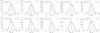 |
Fig. 1 Distribution of IDC values derived from 104 bootstrap simulations (red), each drawn from a sample of size N. The solid vertical line marks the simulated sample mean from Eq. (12). The dashed (green) lines are the curves described by Eq. (7) in the case of a uninformative prior (a = b = 1). |
2. Statistical estimate of the duty cycle
We consider one source for which N independent observations were collected and for which the DC was calculated as described in Sect. 1. In the following we estimate the DC, that we hereafter define as μ, but the formalism is unchanged for the case of the IDC which we consider in Sect. 3. In all generality, the stochastic variable state of the source can be seen as a discrete random variable that can take only one of two possible, mutually exclusive states, active (off) and flaring (on), so that μ is the probability of finding the source active in a given casual pointing. After N observations, the probability of finding the source active m times is given by the binomial 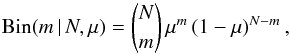 (3)with an expectation value E { m } = μN and variance var{ m } = Nμ(1 − μ). Once N and m are known, where m = Nμest and μest is the DC measured from the N observations, then the problem becomes estimating the statistical offset of μ from μest. From the central limit theorem μest is normally distributed in the limit of large values of m and N − m with E { μest } = μ and
 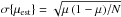 .
.
Hereafter, we adopt a Bayesian treatment, in which μ is treated as a random variable whose probability density function (PDF) depends on the observed values for N and m. From the Bayes theorem, the posterior distribution is proportional to the product of the likelihood and the prior function, and the posterior distribution is to all intents and purposes a PDF of the random variable μ given the observed values for N and m,  (4)where P (m | N,μ) is the likelihood given by Eq. (3) and is meant to be a function of μ. The prior is denoted by p (μ). Apart from a normalization term, the likelihood is the Beta distribution of μ given N and m
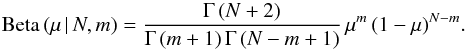 (5)The convenient choice (Bishop 2006, Sect. 2.2.1) for a prior function is a conjugated distribution, which is the Beta distribution with parameters a and b,
 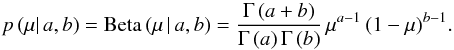 (6)After proper normalization, the posterior in Eq. (4) becomes
 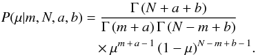 (7)From Eq. (7) the expectation value and variance of μ are
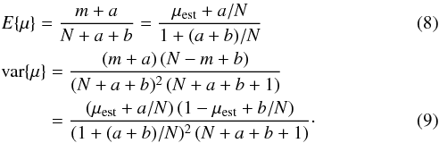 The case of an uninformative prior is easily recovered for a = b = 1. We note that in the asymptotic limit of large values of N,
 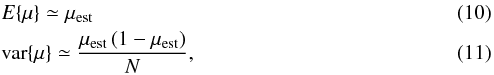 in agreement with the asymptotic limit of a normal distribution.
For a class of sources consisting of a small number of individuals (Nsrc ≲ 50) the prior p (μ) is unknown, so only an uninformative prior can be used in Eq. (4). Such is the case of SFXTs (Nsrc = 10), which will be detailed in Sect. 3, and for which Eq. (7) can only be used with a = b = 1.
To this end, we provide R–language, IDL, and C–language programs that, given N and DC as calculated according to Eq. (2), provide the 68.3%, 95.4%, and 99.7% c.i. for the theoretical distribution (Eq. (7)).
On the contrary, when Nsrc> 50 the prior can be obtained from the observed distribution of the DCs of all sources by fitting it with the Beta function in Eq. (6) with free parameters a and b. In this case, Eq. (6) turns out to be particularly useful for the newly discovered sources even with relatively few available observations. Through the prior, one can further constrain the DC of a new source by exploiting the information (the fitted values of a and b) acquired on the DC distribution derived from the sources of the same class previously observed.
3. Evaluating duty cycles with Monte Carlo bootstrap simulations
Once the best available measurement, DC(N), has been obtained from a set of N independent observations, one needs to assess its associated error. The DC determinations obtained by accumulating increasing observing time are not independent; therefore, the dataset cannot be used to directly determine the error on DC. Furthermore, the datasets can be so poor that the hypothesis of normal errors does not apply. The standard approach, also validating a posteriori our derivation in Sect. 2, is to perform Monte Carlo simulations.
As a test case, we consider the Swift/XRT monitoring campaigns on the ten SFXTs reported in Table 1, discussed in full by Romano et al. (2014) who calculate the IDCs according to Eq. (2). Table 1 (Cols. 1–5) reports the main properties of the sample. The data were divided in i) yearly campaigns (Y), a casual sampling of the X-ray light curve of an SFXT at a resolution of Psamp ~ 3–4 d over a ~1–2 yr baseline (for these, Psamp ≳ Porb); and ii) orbital campaigns (O), that sample the light curve intensively with Psamp ≪ Porb so that the phase space is uniformly observed within one (or a few) Porb. Further details can be found in Romano et al. (2014).
In order to determine the expectation value of IDC and its error, we performed Monte Carlo bootstrap simulations (Efron 1979, 1994). We created M = 104 simulated data sets, drawn from the observed sample of size N with a simple sampling (with replacement, or uniform probability). We calculated M values of IDCs (simulated sample) according to Eq. (2). The simulated sample mean and standard variance (Table 1, Col. 9) are
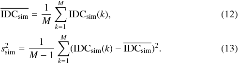
In Fig. 1 we show, superposed on the simulated sample distributions (solid red curves), the simulated sample mean  (vertical line), and the theoretical expectations (dashed green curves) described by Eq. (7). We find that ssim = 2.9–6% for the yearly campaigns and ssim = 8.0–10.4% for the orbital ones.
The standard c.i., defined by the integral of the probability function (i.e. the simulated distributions), the cumulative probability function,  (14)can be calculated from
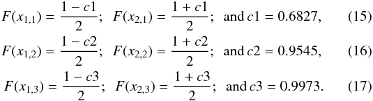
3.1. IDC as a function of sample size
We can now determine the expected IDC value for a given observed sample size via additional Monte Carlo bootstrap simulations. For each of the sources monitored with yearly campaigns, we created M = 104 datasets drawn from the first S = 10,20,30,...,N observed points, with a simple sampling (with replacement, or uniform probability). The simulated sample mean  and the standard deviation sS were calculated similarly to Eqs. (12) and (13).
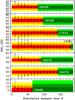 |
Fig. 2 Simulated sample means and their errors |
Figure 2 shows  as a function of the sample size S. The last point (filled triangle) is the simulation for N points for which
  and sN = ssim (Eqs. (12) and (13)). The red-orange-yellow bands mark the 68.3%, 95.4%, and 99.7% c.i. for the simulated distribution as derived from Eqs. (15)–(17). We note the excellent correspondence between the 68.3% c.i. (red band) and the simulated sample standard deviation sN (the error-bar on the simulation for N points), as expected from a normal distribution. The green bands (from dark to light green) mark the 68.3%, 95.4%, and 99.7% c.i. for the theoretical distribution in Eq. (7) also reported in Table 1, Cols. 6–8.
We define Sa as the minimum S value for which IDC(S) is considered acceptable, that is the number of observations required in order to satisfy both conditions: ![Mathematical equation: \begin{eqnarray*} &&\overline{{\rm IDC}_{\rm S}} \in { \left[\overline{{\rm IDC}_{\rm sim}}-s_{\rm sim}, \overline{{\rm IDC}_{\rm sim}}+s_{\rm sim}\right]} \\ &&\overline{{\rm IDC}_{\rm S}}\pm s_{\rm S} \in {\left[\overline{{\rm IDC}_{\rm sim}}-2\,s_{\rm sim}, \overline{{\rm IDC}_{\rm sim}}+2\,s_{\rm sim}\right]} . \end{eqnarray*}](/articles/aa/full_html/2014/12/aa24180-14/aa24180-14-eq96.png) The values of Sa thus determined are reported in Table 1, Col. 10, and they range between 40 and 80 observations, depending on the source.
The values of Sa thus determined are reported in Table 1, Col. 10, and they range between 40 and 80 observations, depending on the source.
Similarly, for each of the sources monitored with orbital campaigns, we created M = 104 datasets drawn from S = 5,10,15,20,...,70 observed points, thus also extrapolating the observed sample to determine how many additional observations are required to significantly lower the uncertainty sS. We find that for about 70 observations sS = 3.6–5.8%, thus comparable to those found for the yearly monitoring campaigns.
These findings can easily be used for planning future observations.
4. Conclusions
As an alternative and considerably less time-consuming approach than Monte Carlo bootstrap simulations, we derived the theoretical Bayesian expectation value for a duty cycle and its error based on a finite set of independent observational data points. We have applied our findings to the specific case of the inactivity duty cycle of SFXTs, as one of the available examples of two-state sources. For SFXTs we have compared the theoretical expectations with both the observed values and with the IDCs and their errors obtained from Monte Carlo simulations, as an a posteriori validation of the Bayesian treatment.
Our treatment, however, is more general than the simple case we considered and can be applied to all independent observations of two-state sources, such as AGNs, X-ray binaries, etc., suitable for a meaningful DC determination. In particular, the strength of this approach becomes evident when considering a well-populated class of sources (Nsrc ≥ 50) for which, the parameters a and b can be obtained by fitting the distribution of the observed DCs for all sources in the class with the Beta function in Eq. (6), thus fully characterizing the prior. Then, whenever a new source in the same class is observed for relatively few observations, the knowledge of the prior derived from the whole class can be utilized to further constrain the DC of this still poorly studied individual source by adopting the a and b of the class.
Acknowledgments
We thank A. Stamerra, P. Esposito, V. Mangano, and E. Bozzo for helpful discussions. C.G. acknowledges PRIN MIUR project on “Gamma Ray Bursts: from Progenitors to Physics of the Prompt Emission Process”, PI: F. Frontera (Prot. 2009 ERC3HT). L.D. thanks Deutsches Zentrum für Luft und Raumfahrt (Grant FKZ 50 OG 1301). We also thank the referee for comments that helped improve the paper. The Swift/XRT data were obtained through target of opportunity observations (2007-2012; contracts ASI-INAF I/088/06/0, ASI-INAF I/009/10/0) and through contract ASI-INAF I/004/11/0 (2011-2013, PI P. Romano).
References
- Ackermann, M., Ajello, M., Allafort, A., et al. 2011, ApJ, 743, 171 [NASA ADS] [CrossRef] [Google Scholar]
- Bishop, C. M. 2006, Pattern Recognition and Machine Learning, eds. M. Jordan, J. Kleinberg, & B. Scholkopf (Springer) [Google Scholar]
- Burrows, D. N., Hill, J. E., Nousek, J. A., et al. 2005, Space Sci. Rev., 120, 165 [NASA ADS] [CrossRef] [Google Scholar]
- Efron, B. 1979, Annals of Statistics, 7, 1 [Google Scholar]
- Efron, B. 1994, An introduction to the bootstrap (New York: Chapman & Hall) [Google Scholar]
- Fragos, T., Kalogera, V., Willems, B., et al. 2009, ApJ, 702, L143 [NASA ADS] [CrossRef] [Google Scholar]
- Gehrels, N., Chincarini, G., Giommi, P., et al. 2004, ApJ, 611, 1005 [NASA ADS] [CrossRef] [Google Scholar]
- Henry, G. R., & Paik, H.-J. 1969, Nature, 224, 1188 [NASA ADS] [CrossRef] [Google Scholar]
- Jorstad, S. G., Marscher, A. P., Mattox, J. R., et al. 2001, ApJ, 556, 738 [NASA ADS] [CrossRef] [Google Scholar]
- Knevitt, G., Wynn, G. A., Vaughan, S., & Watson, M. G. 2014, MNRAS, 437, 3087 [NASA ADS] [CrossRef] [Google Scholar]
- R Core Team 2014, R: A Language and Environment for Statistical Computing (Vienna: R Foundation for Statistical Computing) [Google Scholar]
- Romano, P., Sidoli, L., Cusumano, G., et al. 2009, MNRAS, 399, 2021 [NASA ADS] [CrossRef] [Google Scholar]
- Romano, P., Ducci, L., Mangano, V., et al. 2014, A&A, 568, A55 [NASA ADS] [CrossRef] [EDP Sciences] [Google Scholar]
- Vercellone, S., Soldi, S., Chen, A. W., & Tavani, M. 2004, MNRAS, 353, 890 [NASA ADS] [CrossRef] [Google Scholar]
All Tables
Source sample properties and comparison of measured IDCs with Bayesian estimates and Monte Carlo simulations.
All Figures
|
Fig. 1 Distribution of IDC values derived from 104 bootstrap simulations (red), each drawn from a sample of size N. The solid vertical line marks the simulated sample mean from Eq. (12). The dashed (green) lines are the curves described by Eq. (7) in the case of a uninformative prior (a = b = 1). |
| In the text | |
|
Fig. 2 Simulated sample means and their errors |
| In the text | |
Current usage metrics show cumulative count of Article Views (full-text article views including HTML views, PDF and ePub downloads, according to the available data) and Abstracts Views on Vision4Press platform.
Data correspond to usage on the plateform after 2015. The current usage metrics is available 48-96 hours after online publication and is updated daily on week days.
Initial download of the metrics may take a while.