© ESO, 2014

1. Introduction

Observing stellar occultations caused by different solar system bodies is a powerful technique for obtaining accurate sizes and shapes of these objects and for constraining their atmospheric conditions, if they possess an atmosphere. Theoretically, the technique is simple: The lightcurve of the to-be-occulted star is measured before, during, and after the moving object crosses the star’s line of sight. By precisely measuring the immersion and emersion times of the shadow cast upon Earth and knowing the apparent rate of movement, it is then possible to derive the size of that chord on the moving object, in distance units. Several such chords measured from different locations on Earth allow us to obtain the shape of the body. Furthermore, by analyzing the shape of the lightcurves we can infer whether the object had an atmosphere.

Although occultations of stars by trans-Neptunian objects (TNOs) are quite frequent, it is extremely difficult to predict the exact location of such events, because highly accurate ephemerides and reference star coordinates are necessary. First-order guesses can be made using stellar catalog data and the available ephemerides, but these predictions must be refined. Our group has developed a method for high-precision relative astrometry (see Ortiz et al. 2011) that allows an accurate prediction of the shadow path of the moving object and planning of an observing campaign that involves as many telescopes as possible to increase the chances of positive detections. A side product of such a large campaigns is to enhance the collaboration between professional and amateur astronomers, although in many cases the stars involved are too faint for amateur equipment.

Knowing the sizes of TNOs is fundamental for understanding their evolution, possible composition, and internal structure. Observational surveys obtain magnitudes that can be translated into sizes (e.g., Petit et al. 2008), but, this approach relies on assumptions about the albedo of the objects. Thermal data, on the other hand, can help overcome this problem by obtaining values of albedo and diameters for selected targets (for instance, the successful “TNOs are cool”, one of Herschel Space Observatory’s key projects, Müller et al. 2009) via thermal models. Unfortunately, obtaining thermal measurements of TNOs is extremely challenging, even more so than for asteroids because the thermal emission peak of TNOs is in the submillimetric range and they are usually very faint.

In addition, although thermal models are extremely useful, they have a series of free parameters to be obtained from the fits and no constraints on the shape can be obtained. Thus equivalent diameters and albedos of TNOs are not usually known with a precision better than 10% (e.g., Vilenius et al. 2012). Nevertheless, good precision can in principle be attained for bright and/or closer objects (Fornasier et al. 2013; Duffard et al. 2014). Independent measurements of the diameters from stellar occultations helps to better constrain and understand these free parameters. Another technique to obtain data on TNOs is spectroscopy. But although a spectrum provides a glimpse of the surface composition, it reveals little about the inner composition or structure; this can only be achieved with an accurate knowledge of densities.

Occultations thus provide a unique opportunity of measuring highly accurate sizes, and together with rotational information, for instance, can place strong constraints on densities (e.g., Ďurech et al. 2011). These densities can help to establish whether size distribution of the TNOs for bodies larger than 100 km is indeed primordial, although it might be affected by collisional evolution (Campo-Bagatin & Benavidez 2012 and references therein).

We here describe an occultation event of the NOMAD star 0677-0461184 (α = 16^h35^m04.279^s, δ = −22°15′22.75′′ (J2000.0), B − V = 1.98, V = 17.740, V − R = −0.58, and V − K = 2.49) by the TNO (119951) 2002 KX₁₄. The event was predicted to occur during the first hours of April 26, 2012, and it was especially well suited for the Canary Islands (Spain) observatories.

Throughout we assume the star to be a point source. Unfortunately, not much information exists about the star. Neither its distance, spectral type, or angular diameter are known. According to the calibration of angular diameter versus V − K constructed by van Belle (1999), however, the star probably does not have an angular diameter larger than 0.005 milliarcseconds (mas) or 2.3 × 10^-11 rad if it is a giant star, and the angular diameter is even smaller if it is a main-sequence star. As we will show below, this angular diameter is much smaller than the angular diameter subtended by the TNO. Therefore, assuming that the star is a point source is valid.

The article is organized as follows: First we present the occulting TNO. Section 2 then describes the observations obtained, Sects. 3 and 4 report the results and the method employed to set constraints on the size of the TNO. These results are discussed in Sect. 5, and we conclude in Sect. 6.

1.1. (119951) 2002 KX₁₄

The TNO (119951) 2002 KX₁₄, kx14 hereafter, is a low-inclination (0.4°), low-eccentricity (0.04), classical TNO (see Gladman et al. 2008) orbiting at 38.7 AU, and is one of the brightest TNOs. It has a featureless red visible spectrum (V − R = 0.61, DeMeo et al. 2009; Romanishin et al. 2010) with a spectral slope of 27.1 ± 1.0% (0.1 μm)^-1 (Alvarez-Candal et al. 2008). The near-infrared spectrum is flat with no evident features above the noise (Barkume et al. 2008; Guilbert et al. 2009) and with a possible low water ice content. In Fig. 1 we show the composite spectrum of kx14. As there are no reported NIR colors in the literature, we somewhat arbitrarily scaled scaled the NIR spectrum to match the visible spectrum.

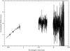Fig. 1 Composite visible-to-near-infrared spectrum of kx14 from Alvarez-Candal et al. (2008) and Guilbert et al. (2009). The spectrum is normalized at 0.55 μm. Photometric data from DeMeo et al. (2009) are shown as filled triangles. The infrared spectrum has been placed at an arbitrary reflectance scale because of the lack of near-infrared colors.

The TNO diameter was estimated using thermal data. Using nondetection data from the Spitzer space observatory, Stansberry et al. (2008) estimated a diameter <$\mathrm{561.}{\mathrm{6}}_{-181.5}^{\mathrm{+}\mathrm{219.9}}$ km. Brucker et al. (2009), on the other hand, measured a diameter =$\mathrm{18}{\mathrm{0}}_{-38}^{\mathrm{+}\mathrm{50}}$ km also using Spitzer data, in this case, from detection data. More recently, using Herschel plus Spitzer data, Vilenius et al. (2012) obtained a diameter of 455 ± 27 km assuming a spherical shape. These authors used the same Spitzer data as Brucker et al. (2009), but with an updated ephemeris, which allowed them to obtain more accurate thermal fluxes.

The rotational period of kx14 is not yet known. The TNO lightcurve has a low amplitude, Δm< 0.05 (Benecchi and Sheppard 2013), which, given the large equivalent diameter, indicates a probable McLaurin shape for this body, as is the case for most of the TNOs (Duffard et al. 2009).

2. Observations

We routinely search for potential occultations of NOMAD and UCAC2 stars by all TNOs potentially larger than 400 km. We select the best candidate occultations and carry out astrometric updates to refine some of the predictions. Using our own predictions of the occultation of the star NOMAD 0677-0461184 by kx14, we attempted observing the event from four different telescopes at three observatories in Spain: the Instituto de Astrofísica de Canarias telescope (IAC-80, 0.8 m) and Telescopio Carlos Sánchez (TCS, 1.5 m), both in Tenerife, and the William Herschel Telescope (WHT, 4.2 m) at La Palma, all three in the Canary Islands; and at the 1.2 m telescope at the Calar Alto Observatory in Almeria. For different technical reasons the observations at the two Tenerife telescopes were unsuccessful, while data obtained at Calar Alto did not detect the event, but, the visiting instrument ULTRACAM (Dhillon et al. 2007) at the WHT recorded the event.

ULTRACAM is an instrument that can obtain high temporal resolution images in three different channels, in our case, the filters used were u′,g′, and i′, by means of two dichroics, making it especially well suited for stellar occultations by solar system objects (e.g., Roques et al. 2006). For the kx14 event we set exposure times of 0.265 s, with dead-times of about 25 ms, obtaining more than 4000 frames for a total time span of approximately 17 min. The seeing during the observations was about 1.4′′.

The data were all reduced using standard methods with IRAF¹. Aperture photometry was performed using the task phot on the position of the occulted star plus several field stars to be used as comparison. The obtained lightcurve is shown in Fig. 2. The flux was normalized to the total brightness of the system star plus kx14 before and after the event to show the depth during the occultation, which was about 2 mag. In spite of the excellent time resolution of the lightcurve, no secondary events were detected that might have indicated satellites or rings (e.g., Timerson et al. 2013; Braga-Ribas et al. 2014).

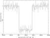Fig. 2 Observed lightcurve in the i′ filter of the system star plus kx14. The total flux before and after the event is normalized to enhance the depth of the event.

The data shown in Fig. 2 were taken using the red arm with the i′ filter, which is the least affected by atmosphere refraction and has the highest signal-to-noise ratio (S/N).

3. Results

We used interactive data language, IDL, routines developed by ourselves to obtain the immersion time, t₀, and the duration of the event, δt from the lightcurve. Both parameters were obtained by fitting a square-well function to the data, allowing the edges to vary and searching for the lowest χ². The results are

${\mathit{t}}_{\mathrm{0}}\mathrm{=}\mathrm{2}\mathrm{h}\mathrm{35}\mathrm{m}\mathrm{1.0}{\mathrm{3}}_{-0.04}^{\mathrm{+}\mathrm{0.05}}\mathrm{s}\mathrm{\left(}\mathrm{UTC}\mathrm{\right)}\mathit{,}\mathrm{and}\mathit{\delta t}\mathrm{=}\mathrm{20.87}\hspace{0.17em}\mathrm{\pm }\hspace{0.17em}\mathrm{0.05}\mathrm{s}\mathit{.}$Using δt and the known rate of the orbital motion, μ = 0.00071 arcsec s^-1, from JPL Horizons², the subtended arc on the sky by the measured chord is (7.200 ± 0.017) × 10^-8 rad. As we know the distance Δ = 38.496 AU from Earth to kx14 and the angle subtended by δt, we can obtain the length of the chord projected upon a plane perpendicular to the line of sight through $\mathit{d}\mathrm{=}\tan \mathrm{[}\mathit{\delta t}\mathrm{\left(}\mathrm{rad}\mathrm{\right)}\mathrm{]}\mathrm{\times }\mathrm{[}\mathrm{\Delta }\mathrm{\left(}\mathrm{km}\mathrm{\right)}\mathrm{]}\mathit{.}$(1)We obtained d = 415 ± 1 km. Note that d is just a distance measured on the object, which corresponds to the shadow cast by the object upon Earth during the occultation and is not necessarily equal to the diameter of kx14. It is a lower limit to the diameter assuming that the object is spherical. The value is consistent within 2-sigma with the equivalent diameter of 455 ± 27 km reported by Vilenius et al.

With only one chord of the occultation observed, it is not possible to place further constraints on the actual size of the object unless pre- or post-occultation astrometric information is available (see one such example for the 1993 occultation of Triton reported by Olkin et al. 1996). Although kx14 was not detected on individual frames, it is possible to detect it in a combined image obtained by stacking the 80 ULTRACAM frames obtained during the occultation when kx14 passed in front of the occulted star, which we call image_d hereafter. We used image_d to measure the photometric centroid of kx14. Similarly, we combined 80 images of the same channel (the i′) before the occultation, and as separated as possible from the time of occultation to minimize contamination by kx14, image_b, and measured the centroid of the star. By doing so we can measure the relative position of the two centroids (kx14−star) in mas on a reference frame oriented with the axes of the detector. We obtained (34,38)_x′y′ mas, with error bars discussed below. We implicitly assumed that kx14 does not possess a detectable atmosphere, otherwise some light from the star would have been detected during the occultation as a result of refraction. This assumption is supported by the sharpness of the lightcurve in Fig. 2.

Below we refer to three different reference frames: detector (x′y′), alt-azimuthal (az), and equatorial (αδ). Indices make self-explanatory in which reference frame the offsets are measured.

Although we attempted to minimize contamination by kx14, the flux of the star in image_b includes the flux of kx14 as well, which affects the centroid position of the star. To evaluate the effect we created a model of kx14 using Chebyshev-Fourier functions (Jiménez-Teja & Benítez 2012) from image_d. This model was subtracted from image_b, taking into consideration the motion of kx14 between the two images, generating image$\begin{array}{c}\mathrm{\prime }\\ \mathit{b}\end{array}$. We measured the difference in the centroids of the star between image_b and image$\begin{array}{c}\mathrm{\prime }\\ \mathit{b}\end{array}$ obtaining (37,25)_x′y′ mas. The difference between the centroids of kx14 and the star is then (−3,13)_x′y′ mas. We stress that these offsets are measured at the moment of closest approach of the star and kx14, that is, at mid-occutlation.

As mentioned, we used the i′ channel of ULTRACAM because it is the least affected by differential chromatic refraction, but it also needs to be corrected. To do this, we used the differential color refraction (DCR) tables provided by Stone (2002). These tables are given for Johnson filters, which have broader wings than the ULTRACAM channels, but, the i′ channel is similar to the Johnson I filter. The corrections depend on the color (B − V) of the object, thus we have to consider the color indices of both the occulted star and kx14, 1.98 and 0.23. In this last case (B − V) was obtained from the spectrum and the known V magnitude (Alvarez-Candal et al. 2008; DeMeo et al. 2009). The corrections are

${\mathrm{DCR}}_{\mathrm{kx}\mathrm{14}\mathrm{-}\mathrm{star}}\mathrm{=}\mathrm{(}\mathrm{0}\mathit{,}\mathrm{6}\mathrm{\pm }\mathrm{1}\mathrm{)}\mathrm{-}\mathrm{(}\mathrm{0}\mathit{,}\mathrm{-}\mathrm{5}\mathrm{\pm }\mathrm{2}\mathrm{)}\mathrm{=}\mathrm{(}\mathrm{0}\mathit{,}\mathrm{11}\mathrm{\pm }\mathrm{2}{\mathrm{)}}_{\mathrm{az}}\mathrm{mas}\mathit{.}$The corrections are given in the alt-azimuthal frame and only affect the zenith distance, thus we projected the DCR onto the detector frame using the position (16°) and parallactic (15.8°) angles, that is,

${\mathrm{DCR}}_{{\mathit{x}}^{\mathrm{\prime }}{\mathit{y}}^{\mathrm{\prime }}}\mathrm{=}{\mathrm{DCR}}_{\mathrm{az}}\mathrm{\times }\sin \mathrm{(}{\mathrm{16}}^{\mathrm{◦}}\mathrm{+}{\mathrm{15.8}}^{\mathrm{◦}}\mathrm{)}\mathrm{=}\mathrm{(}\mathrm{8}\mathrm{\pm }\mathrm{1}\mathit{,}\mathrm{12}\mathrm{\pm }\mathrm{2}\mathrm{)}\mathrm{mas}\mathit{.}$

As the tables are given for a zenith distance of 45°, we scaled to the zenith distance of the observation, z = 52.8°, by multiplying by $\frac{\tan \mathit{z}}{\tan {\mathrm{45}}^{\mathrm{◦}}}\mathrm{·}$ Finally, correcting (−3,13)_x′y′ mas by the DCR _{x′ y′} , we obtain that the offsets of the centroids between kx14 and the star are (−11,0)_x′y′ mas at mid-occultation.

To assess the error in our measurements we simulated observations with varying S/N and full width at half maximum, FWHM. To do this, we extracted the point spread function of a star in one of the stacked images and created images with a S/N varying from 1.0 up to 198.0 for four different values of FWHM: 0.5′′, 1.0′′, 1.5′′, and 2.0′′ using the same plate scale as the original image of 300 mas pix^-1. We measured the centroids using the imexamine task of IRAF for each series and analyzed the effect that S/N and FWHM have on the precision. Figure 3 shows the offsets in the x′y′-space measured with respect to that of the highest S/N image. It is apparent that the lower the S/N, the larger the scatter, and consequently the lower the precision, while the changing FWHM seems to have no systematic effect on the precision. Note that there are no obvious differences between the measurements on the x′ or y′ axes; we consider them to be equal throughout. From the S/N of the star in the stacked image of 25 and the S/N of kx14 of 10 (vertical lines in Fig. 3), their estimated errors are 5 and 10 mas, which accounts for an error in the relative centroid position of 11 mas for x′ and y′.

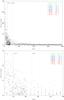Fig. 3 Simulation of centroid positions measured in the x′y′ frame relative to the highest S/N image per FWHM series. Different colors indicate different FWHM. The vertical lines indicate the S/N for kx14 and the occulted star in the stacked images. Top panel: the whole sample. Bottom panel: zoom to the inner zone for clarity.

The final step is to project the corrected shifts to the αδ system through the position angle. The final offsets measured between kx14 and the star centroids are (3 ± 11,10 ± 11)_αδ mas. It is reasonable to assume that these offsets are in fact offsets between the physical center of kx14 and the position of the star. In this case, the center of the shadow-path, mid-occultation, corresponds to the position of the star. Thus now we have a new distance measured: that between the center of the shadow-path (equal to d/ 2) and the center of kx14. We call this distance D = 292 ± 307 km. Note that this distance forms an angle of θ = 73 ± 60° with respect to d (see Fig. 4).

If we assume that the shape of kx14 at the time of the occultation can be described by an ellipsoid, which corresponds to an ellipse projected onto the plane perpendicular to the line of sight, then we now have three points of the ellipse: two corresponding to the extremities of d and its center. Below, however, we see that this information is not enough to unequivocally define the ellipse. With this information we impose constraints on the semi-axes of the ellipse and, consequently, on the equivalent diameter of the ellipsoid in the next subsections. We use the expression “equivalent diameter” (d_eq) to mean equivalent projected area of a sphere, not the equivalent volume. We assume, based on the empirical findings shown in Fig. S7 in Ortiz et al. (2012), that the density of kx14 is 800 kg m^-3 because its expected diameter is probably about 400 km.

4. Analytical development

Figure 4 shows a schematic of the scenario briefly described above. The angle α is, unfortunately, unknown. Nevertheless, we can assume the angle to be known, parameterize the equations, and solve them numerically to estimate the semi-axes of the ellipse.

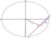Fig. 4 Geometric schematics showing all parameters used in Eqs. (2)−(9). The scale is arbitrary and the angles, and distances are exaggerated for clarity. The star-symbol indicates the position of the occulted star at mid-occultation. The x- and y-axes are aligned with the axes of the ellipse.

We first obtain the position of the two points on the ellipse, P1 and P2, as a function of the parameters shown in Fig. 4 to impose the ellipse to pass over them later on.

We assume this α is known, then we can write the vector D joining the center of the ellipse with the midpoint of the chord P1P2 as ${D}\mathrm{=}\mathrm{\left(}\mathit{D}\cos \mathit{\alpha ,D}\sin \mathit{\alpha }\mathrm{\right)}\mathit{.}$(2)We write the vector V from this midpoint to P1 on the ellipse in terms of θ, d, and α: ${V}\mathrm{=}\frac{\mathit{d}}{\mathrm{2}}\mathrm{\left(}\cos \mathrm{(}\mathit{\alpha }\mathrm{\pm }\mathit{\theta }\mathrm{)}\mathit{,}\sin \mathrm{(}\mathit{\alpha }\mathrm{\pm }\mathit{\theta }\mathrm{)}\mathrm{\right)}\mathit{.}$(3)Using Eqs. (2) and (3), we derive the coordinates of P1 and P2: $\begin{array}{c}\\ {P}{1}\mathrm{=}{D}\mathrm{+}{V}\mathrm{=}\mathrm{(}\mathit{D}\cos \mathit{\alpha }\mathrm{+}\frac{\mathit{d}}{\mathrm{2}}\cos \mathrm{(}\mathit{\alpha }\mathrm{\pm }\mathit{\theta }\mathrm{)}\mathit{,D}\sin \mathit{\alpha }\mathrm{+}\frac{\mathit{d}}{\mathrm{2}}\sin \mathrm{(}\mathit{\alpha }\mathrm{\pm }\mathit{\theta }\mathrm{)}\mathrm{)}\\ {P}{2}\mathrm{=}{D}\mathrm{-}{V}\mathrm{=}\mathrm{(}\mathit{D}\cos \mathit{\alpha }\mathrm{-}\frac{\mathit{d}}{\mathrm{2}}\cos \mathrm{(}\mathit{\alpha }\mathrm{\pm }\mathit{\theta }\mathrm{)}\mathit{,D}\sin \mathit{\alpha }\mathrm{-}\frac{\mathit{d}}{\mathrm{2}}\sin \mathrm{(}\mathit{\alpha }\mathrm{\pm }\mathit{\theta }\mathrm{)}\mathrm{)}\mathit{.}\end{array}$(4)As P1 and P2 belong to the ellipse, they must satisfy the equation $\frac{{\mathit{x}}^{\mathrm{2}}}{{\mathit{a}}^{\mathrm{2}}}\mathrm{+}\frac{{\mathit{y}}^{\mathrm{2}}}{{\mathit{b}}^{\mathrm{2}}}\mathrm{=}\mathrm{1}\mathit{,}$(5)where the center of the ellipse is (0,0) since we have assumed it to match the coordinate origin, and a and b are the semi-major and semi-minor axes of the ellipse, which are the parameters we wish to constrain.

Substituting the expression for P1 and P2 (Eq. (4)) into Eq. (5) and re-arranging terms yields $\begin{array}{c}\\ \mathit{a}\mathrm{=}\frac{\sqrt{\mathrm{2}}}{\mathrm{4}}\\ \hspace{0.17em}\hspace{0.17em}\hspace{0.17em}\mathrm{\times }\sqrt{\mathrm{cosec}\hspace{0.17em}\mathit{\alpha }\hspace{0.17em}\mathrm{cosec}\mathrm{\left(}\mathit{\alpha }\mathrm{\pm }\mathit{\theta }\mathrm{\right)}\sin \mathit{\theta }\mathrm{[}\mathrm{\pm }\mathrm{4}{\mathit{D}}^{\mathrm{2}}\sin \mathrm{2}\mathit{\alpha }\mathrm{\mp }{\mathit{d}}^{\mathrm{2}}\sin \mathrm{(}\mathrm{2}\mathrm{(}\mathit{\alpha }\mathrm{\pm }\mathit{\theta }\mathrm{)}\mathrm{\left)}\mathrm{\right]}}\\ \mathit{b}\mathrm{=}\frac{\sqrt{\mathrm{2}}}{\mathrm{4}}\sqrt{\sec \mathit{\alpha }\sec \mathrm{\left(}\mathit{\alpha }\mathrm{\pm }\mathit{\theta }\mathrm{\right)}\sin \mathit{\theta }\mathrm{[}\mathrm{\mp }\mathrm{4}{\mathit{D}}^{\mathrm{2}}\sin \mathrm{2}\mathit{\alpha }\mathrm{\pm }{\mathit{d}}^{\mathrm{2}}\sin \mathrm{(}\mathrm{2}\mathrm{(}\mathit{\alpha }\mathrm{\pm }\mathit{\theta }\mathrm{)}\mathrm{\left)}\mathrm{\right]}}\mathit{.}\end{array}$(6)

4.1. Numerical solutions

We use the previous mathematical development to obtain values of the semi-axes. We start by directly using Eq. (6) with different values of α while fixing D and θ to their nominal values. Second, we use again Eq. (6), but allowing D and θ to vary within their error bars.

First:

starting from Eq. (6), we obtain values of a and b by allowing α to vary between 0 and 90° in steps of 1° while keeping D and θ fixed at their nominal values. Values in the range α ∈ [ 91°,180°) are also mathematically correct, but provide solutions such that b>a, which have no physical meaning. Equations (6) were then used to derive the values of a and b such that the ratio a/b is minimal. This minimization ensures that the shape we obtain is the least elliptical one. We do this to determine whether the least elliptical shape is still feasible or not.

The results are a = 406 ± 1 km, b = 302 ± 1 km, for α_m = 37° with an equivalent diameter 700 ± 2 km. Note that a/b is larger than 1.3, indicating a rotational period of about 9 h for a density of 800 kg m^-3 (see Fig. A.1) assuming a hydrostatic equilibrium shape. We regard this solution as unlikely since the size obtained of kx14 is much larger than the best solutions found by thermal modeling (Sect. 1.1).

Second:

we allow D and θ to vary within their errors (± σ) on an equally spaced grid of 201 × 201 points, that is, ${\mathit{D}}_{\mathit{i}}^{\mathrm{\prime }}\mathrm{=}\mathit{D}\mathrm{+}\mathit{i}\mathrm{\ast }\mathit{\sigma }\mathit{/}\mathrm{200}$, i = −100, −99...,99,100, likewise for θ. The only imposed condition is that ${\mathit{D}}_{\mathit{i}}^{\mathrm{\prime }}\mathrm{\ge }\mathrm{0}$ km. As before, α ranges from 0° to 90° in steps of 1°. This approach provides us with slightly fewer than 90 × 201 × 201 solutions.

To simplify the search for solutions we searched for the most frequent values of a/b. We created a histogram of a/b in bins of 0.005 and searched for the maximum of the distribution. As we proposed that kx14 can be well described by a Maclaurin spheroid, we only retained values with that ratio higher than 1.1 (see Appendix A). The results are shown in Fig. 5.

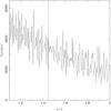Fig. 5 Histogram of a/b in bins of 0.005, shown only for values higher than 1.1 (see Appendix A), following Sect. 4.1. The vertical line indicates the value a/b = 1.45 that halves the sample.

There is a clear trend to decrease the number of occurrences with increasing a/b, with a median value of a/b = 1.45 (marked with a vertical line in Fig. 5). We searched for the solution in the region that holds 50% of the sample with the lower value of a/b, aiming at the least elliptical solutions. Therefore the solutions we consider valid lie within 1.1 ≤ a/b ≤ 1.45. The median value a = 409.41 km implies an equivalent diameter over 700 km, even for a/b = 1.1. In view of the Herschel result (455 km, Vilenius et al. 2012), we prefer solutions with lower values of a. Therefore, we select the lowest value of a in the interval 1.1 ≤ a/b ≤ 1.45, which is 207.54 km, with a corresponding a/b = 1.29, resulting in ${\mathit{d}}_{\mathrm{eq}}\mathrm{=}\mathrm{36}{\mathrm{5}}_{-21}^{\mathrm{+}\mathrm{30}}$ km.

The error bars in d_eq we estimated by assuming a fixed at 207.54 km and computing equivalent diameters for a/b = 1.1 and 1.45, which provide upper and lower limits to d_eq. The ellipse is shown in Fig. 6 and, according to the appendix, it corresponds to a rotational period of ~9 h, assuming an equatorial view.

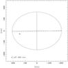Fig. 6 Resulting ellipse obtained for the second step in Sect. 4.1 corresponding to deq = 365 km. All distances are correctly scaled. The dashed line indicates the measured chord.

4.2. Constraining α

The only unknown parameter in the previous discussion (Sect. 4) was α. If we had an additional observational constraint, we would be able to remove any ambiguity and solve the system shown in Eqs. (6) to obtain the shape of kx14. To do this, we used as an additional boundary condition the equivalent diameter, d_eq = 455 ± 27 km, as given by Vilenius et al. (2012). The areas of this equivalent circumference and our ellipse, which is a two-dimensional projection onto the plane perpendicular to the line of sight of the actual volume, must coincide so that $\mathit{\pi }\mathrm{(}{\mathit{d}}_{\mathrm{eq}}\mathit{/}\mathrm{2}{\mathrm{)}}^{\mathrm{2}}\mathrm{=}\mathit{\pi ab,}$(7)and thus, $\tan \mathrm{2}\mathit{\alpha }\mathrm{=}\frac{\sin \mathrm{2}\mathit{\theta }}{\mathit{f}\mathrm{\left(}{\mathit{d}}_{\mathrm{eq}}\mathit{,d,D,\theta }\mathrm{\right)}\mathrm{-}\cos \mathrm{2}\mathit{\theta }}\mathit{,}$(8)where the function f is defined by $\begin{array}{c}\\ \mathit{f}\mathrm{\left(}{\mathit{d}}_{\mathrm{eq}}\mathit{,d,D,\theta }\mathrm{\right)}\mathrm{=}\frac{\mathrm{1}}{\mathrm{2}{\mathit{d}}^{\mathrm{4}}}\\ \mathrm{\times }\left[\mathrm{8}{\mathit{d}}^{\mathrm{2}}{\mathit{D}}^{\mathrm{2}}\mathrm{-}{\mathit{d}}_{\mathrm{eq}}^{\mathrm{4}}\hspace{0.17em}\mathrm{cosec}\hspace{0.17em}{\mathit{\theta }}^{\mathrm{2}}\hspace{0.17em}\mathrm{\pm }\hspace{0.17em}\mathrm{cosec}\hspace{0.17em}\mathit{\theta }\hspace{0.17em}\sqrt{{\mathit{d}}_{\mathrm{eq}}^{\mathrm{8}}\mathrm{cosec}\hspace{0.17em}{\mathit{\theta }}^{\mathrm{2}}\mathrm{-}\mathrm{16}{\mathit{d}}^{\mathrm{2}}{\mathit{D}}^{\mathrm{2}}{\mathit{d}}_{\mathrm{eq}}^{\mathrm{4}}}\right]\mathit{.}\end{array}$(9)By computing following the scheme d_eq,d,D,θ → f(d_eq,d,D,θ) → α → a,b we obtain the semi-axes. Note that the only additional assumption introduced here is the measurement of the equivalent diameter by Vilenius et al.

Third:

Given the extra constraint d_eq measured by Vilenius et al. (2012), and as we know D and θ, it follows that α is fully determined, but not necessarily a real number. This is the case for the nominal values of D and θ. Moreover, as can be seen from Eq. (9), complex solutions occur whenever $\mathrm{16}{\mathit{d}}^{\mathrm{2}}{\mathit{D}}^{\mathrm{2}}\mathit{>}{\mathit{d}}_{\mathrm{eq}}^{\mathrm{4}}\mathrm{cosec}\hspace{0.17em}\mathit{\theta }2$(10)is satisfied.

Fourth:

Similarly to before, we now allow D and θ to vary within their error bars.

Fig. 7 Histogram of a/b in bins of 0.005, shown only for values higher than 1.1 (see Appendix A), following Sect. 4.2. A clear maximum in the distribution appears at a/b = 1.203.

Using only the real solutions of α, we created the histogram of a/b (Fig. 7). In this case, because we provide an additional constraint, there is a clear maximum at a/b = 1.203. Again, there are several values of a that fall within that bin, therefore we select, as before, the median value of a = 249 ± 1 km with a a/b = 1.20. The corresponding value of $\mathit{b}\mathrm{=}\mathrm{20}{\mathrm{8}}_{-5}^{\mathrm{+}\mathrm{4}}$ km (Fig. 8). From this we recover the diameter as $\mathrm{45}{\mathrm{5}}_{-6}^{\mathrm{+}\mathrm{5}}$ km. Assuming a density of 800 kg m^-3, the rotational period probably is about 11 h.

Fig. 8 Resulting ellipse obtained in the fourth approach in Sect. 4.2. All distances are correctly scaled. The dashed line indicates the measured chord.

5. Discussion

The results described in Sect. 4 indicate that the equivalent diameter of kx14 lies between a minimum of $\mathrm{36}{\mathrm{5}}_{-21}^{\mathrm{+}\mathrm{30}}$ km and 455 ± 27 km from Vilenius et al. (2012). The low lightcurve amplitude, lower than 0.05 mag, rules out an irregularly shaped body (which was not expected because of the large size of the object). Unfortunately, we cannot constrain the density of kx14 because the rotational period is not determined. Nevertheless, using a reasonable estimate of the density of 800 kg m^-3 (see Fig. S7 from Ortiz et al. 2012, supplementary information) and assuming a Maclaurin spheroid, we can constrain a rotational period of between 9 and 11 h. This remains to be confirmed, but is in the typical range for most observed TNOs (e.g., Thirouin et al. 2012) and is therefore quite plausible.

The data presented in Fig. 2 do not show evidence of a developed atmosphere because the drops at immersion and emersion are quite sharp. This is consistent with the featureless spectrum shown in Fig. 1, in which no clear evidence of very volatile ice is present within the noise. According to the volatile retention model of Schaller & Brown (2007), it is very unlikely that kx14 has retained volatiles older than the age of the solar system. With the estimate of the size given in this work the effective temperature of kx14 is probably below 30 K for it to have retained at least methane-ice.

Using the published value of the absolute magnitude H_V = 4.86 ± 0.1 (Vilenius et al. 2012), we can invert the well-known relationship between geometric albedo in the visible, p_V, and $\mathrm{diameter}\mathrm{\left(}\mathrm{km}\mathrm{\right)}\mathrm{=}\frac{\mathrm{1.329}}{\sqrt{{\mathit{p}}_{\mathit{V}}}}\mathrm{\times }{\mathrm{10}}^{\mathrm{3}\mathrm{-}\frac{{\mathit{H}}_{\mathit{V}}}{\mathrm{5}}}\mathit{,}$(11)to obtain a value of albedo. For the smallest equivalent diameter provided here, $\mathrm{36}{\mathrm{5}}_{-21}^{\mathrm{+}\mathrm{30}}$ km, we obtain ${\mathit{p}}_{\mathit{V}}\mathrm{=}\mathrm{0.1}{\mathrm{5}}_{-0.03}^{\mathrm{+}\mathrm{0.04}}$.

Using this albedo, it is now possible to estimate the effective temperature of kx14. We use ${\mathit{T}}_{\mathrm{eff}}\mathrm{=}[\frac{\mathrm{(}\mathrm{1}\mathrm{-}\mathit{A}\mathrm{)}{\mathit{S}}_{\mathrm{\odot }}}{\mathit{ϵ\eta \sigma \chi }{\mathit{r}}^{\mathrm{2}}}{]}^{\mathrm{0.25}}\mathit{,}$(12)where A is the bond albedo and can be approximated by qp_V, the phase integral is q = 0.366p_V + 0.479 (from Vilenius et al. 2012). The heliocentric distance is r = 39.331 AU. The other values are the solar constant S_⊙ = 1360 Wm^-2, the emissivity ϵ = 0.9 (usual approximation for solar system objects, Hovis & Callahan 1966), the Boltzmann constant σ = 5.67 × 10^-8 Wm^-2K^-4, and the beaming factor $\mathit{\eta }\mathrm{=}\mathrm{1.7}{\mathrm{9}}_{-0.15}^{\mathrm{+}\mathrm{0.16}}$ (Vilenius et al. 2012). The last factor, χ, depends on the rotation of the object: χ = π for fast rotators or χ = 2 for slow rotators. Introducing all the parameters in the equation above, we obtain obtain T_eff = 41 ± 1 K for a fast rotator, or T_eff = 46 ± 1 K for a slow rotator. Both values are consistent with the picture drawn above, and we do not expect very volatiles ices on kx14 that could give rise to an atmosphere.

For a diameter of $\mathrm{45}{\mathrm{5}}_{-6}^{\mathrm{+}\mathrm{5}}$ km we obtain p_V = 0.10 ± 0.01 and the same temperatures for the slow and fast rotator case.

The lack of water ice in its spectrum, or very tiny amounts of it, is consistent with the low albedo because water ice patches on its surface would increase the albedo.

6. Conclusions

Using data from a stellar occultation by (119951) 2002 KX₁₄ of April 2012, we obtained a chord of 415 ± 1 km. In spite of lacking other measured chords of the event, we were able to establish reasonable constraints of the size, d_eq between 365 and 455 km using astrometric information at the time of the occultation. This was possible by assuming an elliptical shape for the projected shape of kx14 during the occultation, which is supported by the fact that most large TNOs with small, almost null, lightcurve amplitude have acquired relaxed hydrostatic figures, in this case, a Maclaurin shape.

We developed a method for obtaining an equivalent diameter from single-chord occultations by a combination of (i) accurate astrometry carried out on stacked images during the event; (ii) analytically finding the equations to express the semi-axes in terms of the known quantities; and (iii) numerically solving the equations to obtain values for the semi-axes.

The lightcurve does not reveal the existence of a Pluto-like atmosphere on the TNO. Moreover, the estimated effective temperature is high enough to predict that the surface of kx14 is already depleted of the most volatile ices and probably cannot have a developed atmosphere.

Acknowledgments

A.A.C. acknowledges support from the Marie Curie Actions of the European Commission (FP7-COFUND), FAPERJ, and CNPq. J.L.O. acknowledges funds from Spanish MINECO grant AYA2011-30106-C02-01. Y.J.T. acknowledges funds from CAPES through the “Science Without Borders” program. R.D. acknowledge the support of MINECO for his Ramón y Cajal Contract. S.L., V.S.D., T.M. and ULTRACAM are supported by the STFC. T.S. supported by the Spanish Ministry of Economy and Competitiveness (MINECO) under the grant (project reference AYA2010-18080). The authors acknowledge the comments by an anonymous referee that improved the quality of this manuscript.

References

Appendix A: Maclaurin spheroid

A Maclaurin spheroid is the figure of a body in hydrostatic equilibrium that is rotationally symmetric about its rotation axis. Thus, when viewed pole-on, its shape is a circle of radius a, while viewed side-on, its shape is an ellipse with the semi-major axis a and the semi-minor axis b. According to Fig. 6 in Duffard et al. (2009), most TNOs with densities higher than about 700 kg m^-3 have this shape.

The relationship between the shape of a Maclaurin spheroid and its density (ρ) and rotation period (P) (see Plummer 1919) is $\frac{{\mathit{\omega }}^{\mathrm{2}}}{\mathrm{2}\mathit{\pi }\mathit{G\rho }}\mathrm{=}\frac{\mathrm{3}\mathrm{-}\mathrm{2}{\mathit{e}}^{\mathrm{2}}}{{\mathit{e}}^{\mathrm{3}}}{\mathrm{(}\mathrm{1}\mathrm{-}{\mathit{e}}^{\mathrm{2}}\mathrm{)}}^{\mathrm{0.5}}\arcsin \mathit{e}\mathrm{-}\frac{\mathrm{3}}{{\mathit{e}}^{\mathrm{2}}}\mathrm{(}\mathrm{1}\mathrm{-}{\mathit{e}}^{\mathrm{2}}\mathrm{)}\mathit{,}$(A.1)\\where e = (1 − (b/a)²)^0.5, ω = 2π/P, and G = 6.67 × 10¹¹ Nm² kg^-2 is the gravitational constant. Figure A.1 shows the density plotted against the ratio a/b, the rotational period increases toward the left of the figure. It is clear that for slowly rotating bodies and higher densities, the ratio a/b could reach values of 1, corresponding to a sphere.

We color-coded different period intervals in Fig. A.1 for clarity. We restricted the period range to values between 6 and 12 h to encompass most of the data available for TNOs (Fig. 7 in Duffard et al. 2009). We note that for a density of 800 kg m^-3 the average values of a/b are about 1.2, 1.35, and 1.55 per period interval considered in the figure and in no case lower than 1.1, which would require rotational periods significantly longer than 12 h.

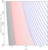Fig. A.1 Density vs. a/b using the rotational period as parameter. Different colors indicate different P-ranges: black (10 <P< 12 h), red (8 <P< 10 h), and blue 6 <P< 8 h.

All Figures

	Fig. 1 Composite visible-to-near-infrared spectrum of kx14 from Alvarez-Candal et al. (2008) and Guilbert et al. (2009). The spectrum is normalized at 0.55 μm. Photometric data from DeMeo et al. (2009) are shown as filled triangles. The infrared spectrum has been placed at an arbitrary reflectance scale because of the lack of near-infrared colors.
In the text

	Fig. 2 Observed lightcurve in the i′ filter of the system star plus kx14. The total flux before and after the event is normalized to enhance the depth of the event.
In the text

	Fig. 3 Simulation of centroid positions measured in the x′y′ frame relative to the highest S/N image per FWHM series. Different colors indicate different FWHM. The vertical lines indicate the S/N for kx14 and the occulted star in the stacked images. Top panel: the whole sample. Bottom panel: zoom to the inner zone for clarity.
In the text

	Fig. 4 Geometric schematics showing all parameters used in Eqs. (2)−(9). The scale is arbitrary and the angles, and distances are exaggerated for clarity. The star-symbol indicates the position of the occulted star at mid-occultation. The x- and y-axes are aligned with the axes of the ellipse.
In the text

	Fig. 5 Histogram of a/b in bins of 0.005, shown only for values higher than 1.1 (see Appendix A), following Sect. 4.1. The vertical line indicates the value a/b = 1.45 that halves the sample.
In the text

	Fig. 6 Resulting ellipse obtained for the second step in Sect. 4.1 corresponding to deq = 365 km. All distances are correctly scaled. The dashed line indicates the measured chord.
In the text

	Fig. 7 Histogram of a/b in bins of 0.005, shown only for values higher than 1.1 (see Appendix A), following Sect. 4.2. A clear maximum in the distribution appears at a/b = 1.203.
In the text

	Fig. 8 Resulting ellipse obtained in the fourth approach in Sect. 4.2. All distances are correctly scaled. The dashed line indicates the measured chord.
In the text

	Fig. A.1 Density vs. a/b using the rotational period as parameter. Different colors indicate different P-ranges: black (10 <P< 12 h), red (8 <P< 10 h), and blue 6 <P< 8 h.
In the text

References

- Alvarez-Candal, A., Fornasier, S., Barucci, M. A., et al. 2008, A&A, 487, 741 [NASA ADS] [CrossRef] [EDP Sciences] [Google Scholar]
- Barkume, K. M., Brown, M. E., & Schaller, E. L. 2008, AJ, 135, 55 [NASA ADS] [CrossRef] [Google Scholar]
- Benecchi, S. D., & Sheppard, S. S. 2013, AJ, 145, 124 [NASA ADS] [CrossRef] [Google Scholar]
- Braga-Ribas, F., Sicardy, B., Ortiz, J. L., et al. 2014, Nature, 508,72 [NASA ADS] [CrossRef] [Google Scholar]
- Brucker, M. J., Grundy, W. M., Stansberry, J. A., et al. 2009, Icarus, 201, 284 [NASA ADS] [CrossRef] [Google Scholar]
- Campo-Bagatin, A., & Benavidez, P. G. 2012, MNRAS, 423, 1254 [NASA ADS] [CrossRef] [Google Scholar]
- DeMeo, F. E., Fornasier, S., Barucci, M. A., et al. 2009, A&A, 493, 283 [NASA ADS] [CrossRef] [EDP Sciences] [Google Scholar]
- Dhillon, V. S., Marsh, T. R., Stevenson, M. J, et al. 2007, MNRAS, 378, 825 [NASA ADS] [CrossRef] [MathSciNet] [Google Scholar]
- Duffard, R. D., Ortiz, J. L., Thirouin, A., et al. 2009, A&A, 505, 1283 [NASA ADS] [CrossRef] [EDP Sciences] [Google Scholar]
- Duffard, R., Pinilla-Alonso, N., Santos-Sanz, P., et al. 2014, A&A, 564, A92 [NASA ADS] [CrossRef] [EDP Sciences] [Google Scholar]
- Ďurech, J., Kaasalainen, M., Herald, D., et al. 2011, Icarus, 214, 652 [NASA ADS] [CrossRef] [Google Scholar]
- Fornasier, S., Lellouch, E., Müller, T. G., et al. 2013, A&A, 555, A15 [NASA ADS] [CrossRef] [EDP Sciences] [Google Scholar]
- Guilbert, A., Alvarez-Candal, A., Merlin, F., et al. 2009, Icarus, 201, 272 [NASA ADS] [CrossRef] [Google Scholar]
- Gladman, B., Marsden, B. G., & VanLaerhoven, C. 2008, Nomenclature in the outer Solar System, in The Solar System Beyond Neptune, eds. M. A. Barucci, H. Boehnhardt, D. Cruikshank, & A. Morbidelli (Tucson: Univ. of Arizona Press), 43 [Google Scholar]
- Hovis, W. A., & Callahan, W. R. 1966, J. Opt. Soc. Am., 56, 639 [NASA ADS] [CrossRef] [Google Scholar]
- Jiménez-Teja, Y., & Benítez, N. 2012, ApJ, 745, id. 150 [Google Scholar]
- Müller, T. G., Lellouch, E., Böhnhardt, H., et al. 2009, Earth Moon and Planets, 105, 209 [CrossRef] [Google Scholar]
- Olkin, C. B., Elliot, J. L., Bus, S. J., et al. 1996, PASP, 108, 202 [NASA ADS] [CrossRef] [Google Scholar]
- Ortiz, J. L., Cikota, A., Cikota, S., et al. 2011, A&A, 525, A31 [NASA ADS] [CrossRef] [EDP Sciences] [Google Scholar]
- Ortiz, J. L., Sicardy, B., Braga-Ribas, F., et al. 2012, Nature, 491, 566 [NASA ADS] [CrossRef] [Google Scholar]
- Petit, J.-M., Kavelaars, J. J., Gladman, B., et al. 2008, Size distribution of multikilometer transneptunian objects, in The Solar System Beyond Neptune, eds. M. A. Barucci, H. Boehnhardt, D. Cruikshank, & A. Morbidelli (Tucson: Univ. of Arizona Press), 71 [Google Scholar]
- Plummer, H. C. 1919, MNRAS, 80, 26 [NASA ADS] [CrossRef] [Google Scholar]
- Romanishin, W., Tegler, S. C., & Consolmagno, G. J. 2010, AJ, 140, 29 [NASA ADS] [CrossRef] [Google Scholar]
- Roques, F., Doressoundiram, A., Dhillon, V., et al. 2006, AJ, 132, 819 [NASA ADS] [CrossRef] [Google Scholar]
- Schaller, E. L., & Brown, M. E. 2007, AJ, 659, L61 [NASA ADS] [CrossRef] [Google Scholar]
- Stansberry, J., Grundy, W., Brown, M., et al. 2008, Physical Properties of Kuiper Belt and Centaur Objects: Constraints form the Spitzer Space Telescope, in The Solar System Beyond Neptune, eds. M. A. Barucci, H. Boehnhardt, D. Cruikshank, & A. Morbidelli (Tucson: Univ. of Arizona Press), 161 [Google Scholar]
- Stone, R. C. 2002, PASP, 114, 1070 [NASA ADS] [CrossRef] [Google Scholar]
- Thirouin, A., Ortiz, J.L., Campo-Bagatin, A., et al. 2012, MNRAS, 242, 3156 [NASA ADS] [CrossRef] [Google Scholar]
- Timerson, B., Brooks, J., Conrad, S., et al. 2013, P&SS, 87, 78 [Google Scholar]
- van Belle, G. T. 1999, PASP, 111, 1515 [NASA ADS] [CrossRef] [Google Scholar]
- Vilenius, E., Kiss, C., Mommert, M., et al. 2012, A&A, 541, A94 [NASA ADS] [CrossRef] [EDP Sciences] [Google Scholar]