| Issue |
A&A
Volume 570, October 2014
|
|
|---|---|---|
| Article Number | A17 | |
| Number of page(s) | 6 | |
| Section | Numerical methods and codes | |
| DOI | https://doi.org/10.1051/0004-6361/201424463 | |
| Published online | 07 October 2014 | |
Genetic algorithm to design Laue lenses with optimal performance for focusing hard X- and γ-rays
Department of Physics and Earth Sciences and INFN-Ferrara, University of Ferrara, via Saragat 1/c, 44122 Ferrara, Italy
e-mail: This email address is being protected from spambots. You need JavaScript enabled to view it.
Received: 24 June 2014
Accepted: 18 August 2014
Abstract
To focus hard X- and γ-rays it is possible to use a Laue lens as a concentrator. With this optics it is possible to improve the detection of radiation for several applications, from the observation of the most violent phenomena in the sky to nuclear medicine applications for diagnostic and therapeutic purposes. We implemented a code named LaueGen, which is based on a genetic algorithm and aims to design optimized Laue lenses. The genetic algorithm was selected because optimizing a Laue lens is a complex and discretized problem. The output of the code consists of the design of a Laue lens, which is composed of diffracting crystals that are selected and arranged in such a way as to maximize the lens performance. The code allows managing crystals of any material and crystallographic orientation. The program is structured in such a way that the user can control all the initial lens parameters. As a result, LaueGen is highly versatile and can be used to design very small lenses, for example, for nuclear medicine, or very large lenses, for example, for satellite-borne astrophysical missions.
Key words: techniques: high angular resolution / telescopes / instrumentation: high angular resolution
© ESO, 2014
1. Introduction
Focalizing hard X- and γ-rays in the 100−1000 keV energy range is a topic of growing interest because of the wealth of physical experiments that could be performed and the technological spin-off that could be derived. Today, observing the photons in this energy range is comparable to old-fashioned naked-eye observations rather than observations with optic-equipped devices because it is impossible to concentrate such high-energy photons. Indeed, the lack of optical components that work in this energy range results in the impossibility of focusing, which in turn means a poor signal-to-noise ratio recorded by the detectors.
One nonfocusing method that has been implemented for several decades for X-ray detection consists of using of geometrical optics, such as collimators or coded masks (e.g. Ubertini et al. 2003). However, since the total interaction cross-section for γ-rays attains its minimum within 100−1000 keV, the efficiency of geometrical optics decreases while at the same time the background noise increases with respect to the signal because of the growing increase of shield leakage and/or nβ activation. Another nonfocusing solution consists of quantum optics based on Compton effect and tracking detectors (e.g. Schonfelder et al. 1984; Von Ballmoos et al. 2005a).
Focusing methods have a greater potential because they can concentrate the signal from a large collector onto a small detector and beat the instrumental background that may hamper the observation. Bragg diffraction can be used to concentrate the signal with high efficiency . As focusing optics, grazing incidence depth-graded multilayer optics have been proven to be capable of focusing up to 80 keV photons with high-efficiency Madsen et al. (2009). More recently, it was demonstrated that multilayer reflective optics can operate efficiently and according to classical-wave physics up to photon energies of at least 600 keV (Fernández-Perea et al. 2013; Brejnholt et al. 2014). However, these new reflective optics work at very low grazing incidence angles, below 0.1°, which means that they have a very low acceptance area for the incident photons, and beyond these energy limits their efficiency critically deteriorates.
If X-ray diffraction occurs in Laue geometry, that is, if traverses the crystals, the hard X-rays can be focused via a Laue lens (Lund 1992). A Laue lens is conceived as an ensemble of many crystals arranged in such a way that as much radiation as possible is diffracted onto the lens focus over a selected energy band (see Fig. 1). A Laue lens can be employed for astrophysical purposes for high-sensitivity observations of many cosmic phenomena. Indeed, X- and γ-ray emissions occur in several places in the Universe, from near solar flares to compact binary systems, pulsars, and supernova remnants within our Galaxy, and finally to extremely distant objects such as active galactic nuclei and γ-ray bursts (GRBs) at redshifts z> 8.
A Laue lens can also be used for high-quality diagnosis in nuclear medicine. For instance, it would improve γ-ray detection in single-photon emission computed tomography (SPECT) and in positron emission tomography (PET) by providing better scan resolution. This, in turn, would lead to a lower radioactive dose being imparted to the patient, since there would be no need for tomography scanning (Roa et al. 2005).
A Laue lens can also be used to concentrate hard X-rays for therapy purposes. Indeed, radiation therapy uses high-energy radiation to kill cancer cells by damaging their DNA. Since the radiation therapy can damage normal cells as well as cancer cells, the treatment must be carefully planned to minimize side effects. With a Laue lens it would be possible to minimize the collateral effects of the radiation therapy and to improve its functionality.
 |
Fig. 1 Schematic representation of a Laue lens. The red arrows represent an X-ray beam that is diffracted toward a detector placed on the focal point of the lens. |
Diffracting crystals are the optical elements of a Laue lens. To date, several materials have been proposed for diffracting X- and γ-rays. The first Laue lens telescope was built by Lindquist, who flew it with a stratospheric balloon in 1967 (Lindquist & Webber 1968). Progress has been made since then, both in the growth of high-quality crystals and in processing them.
To build a high-efficiency Laue lens, the choice and arrangement of the crystals are key points. The diffraction response of crystals in a Laue lens is a function of material, crystallographic orientation, and position of the crystals in the lens. It can be useful to mix different materials and crystallographic orientations for the X-ray diffraction to achieve the highest integrated reflectivity together with smoothing the energy dependence of the collected photons, or in other words, smoothing the lens effective area curve. Smoothing the spectral response is important to simplify the deconvolution of the collected signal, while the high-reflectivity of the optical elements is fundamental to increase the signal-to-noise ratio of the lens.
Since the implementation of a Laue lens may be very expensive, an appropriate simulation of its features before its realization is fundamental. However, the optimized arrangement of the crystals on a Laue lens cannot be approached analytically. A genetic algorithm might be the best method to resolve the problem. A genetic algorithm is a search heuristic that mimics the process of natural selection. With a genetic algorithm, a population of candidate solutions to an optimization problem is evolved toward better solutions. In particular, a Laue lens can be optimized through a pseudo-evolutionistic process. The process favors the usage of the crystals that have the best characteristics, to configure the system with the desired features.
We here propose the LaueGen genetic algorithm is proposed. It is capable of selecting and arranging the crystal tiles in a Laue lens in such a way as to maximize its integrated reflectivity smoothing the energy dependence of the collected photons. In next section we report the description and the theoretical reflectivity of the crystals proposed so far for a Laue lens. Then we describe the code, and finally we give some examples.
2. Crystals for high-efficiency diffraction
To realize a Laue lens, crystals that can diffract the radiation with high efficiency and with a controlled passband response are needed. For this purpose, the scientific community has proposed several types of crystals: mosaic crystals (Zachariasen 1945) and crystals with curved diffracting planes (CDP; Keitel et al. 1999). More recently, a particular optical element based on CDPs has been proposed: the quasi-mosaic (QM) crystal, which has two different curvatures in two lyings of perpendicular planes (Sumbaev 1968). The features of these crystals are quite different, and we describe them in the next subsections.
2.1. Mosaic crystals
A mosaic crystal can be described using Darwin’s model as an assembly of tiny identical small perfect crystals, called crystallites, each slightly misaligned with respect to the others according to an angular distribution, usually taken as Gaussian, spread about a nominal direction (Zachariasen 1945). Misaligned crystallites provide an enlarged bandpass for the diffracted photons. For a mosaic crystal, reflectivity is given by (Barrière et al. 2009) 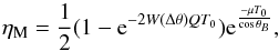 (1)where T0 is the crystal thickness traversed by radiation, Δθ the difference between the angle of incidence and the Bragg angle θB, μ the linear absorption coefficient within the crystal, and W(Δθ) the distribution function of crystallite orientations. In turn, W(Δθ) is defined as
  (2)where ΩM is called mosaicity, or mosaic spread, and represents the full width at half maximum (FWHM) of the angular distribution of the crystallites. Finally, by considering the dynamical theory of diffraction (Malgrange 2002), Q is given by the dynamical theory of diffraction
  (3)where dhkl is the d-spacing of the diffracting planes, and Λ0 the extinction length as defined in Authier (2001) for the Laue symmetric case. For this case, f(A) is given by
  (4)This approximation is always valid for energies above 100 keV because θB is small. B0 is the Bessel function of zero order integrated between 0 and 2A, with A being
  (5)where t0 is the crystallite thickness.
2.2. CDP crystals
Perfect crystals with curved diffracting planes (CDP crystals) represent an alternative to mosaic crystals. The curvature of the diffracting planes results in a very well controlled of the energy bandpass because it is proportional to the angular distribution of the diffracting planes. For CDP crystals, the reflectivity is given by (Malgrange 2002)  (6)where, in this case, ΩC represents the bending angle of the curved diffracting planes. The angular distribution of the diffracting planes WC(Δθ) is a uniform distribution with the width being the angular spread ΩC. It is
  (7)
(7)
2.3. QM crystals
A QM crystal features two curvatures of two different lying of crystallographic planes. As a crystal is bent by external forces, another curvature can be generated within the crystal under very specific orientations. This is the QM curvature. Because of the external curvature, this crystal permits focalizing the radiation on the scattering plane (Guidi et al. 2011). Since QM crystals belong to the CDP class, their reflectivity is given by Eq. (6). However, the angular distribution of the diffracting planes is the convolution between the external and the QM curvature:  (8)Some examples of QM crystals employed for high-focusing diffraction are reported in Camattari et al. (2013, 2014a). For these crystals, the external curvature of the samples (obtained with external forces) has to be the same as that of the lens calotte to guarantee a continuous energy band-pass response. The QM curvature is needed to increase the integrated reflectivity, because this curvature provides CDPs for the photon diffraction.
3. LaueGen algorithm
The particular characteristics of a Laue lens may vary substantially according to the application the lens is needed for. To be general and highly versatile, the program allows the user to set several initial parameters. These parameters are
-
the focal length f;
-
the energy band;
-
the size of the crystals;
-
the smallest and the largest radius of the Laue lens Rmin and Rmax;
-
the material of the crystals (including the type, for instance, mosaic, CDP, or QM);
-
the diffracting planes.
The focal length of a Laue lens for astrophysical purposes can change depending on the structure on which the lens has to be mounted. For example, in the case of a balloon, the focal length must not exceed a few meters (von Ballmoos et al. 2005b). If the lens is launched through a satellite, the focal length may be up to 20 m (Frontera et al. 2012; Virgilli et al. 2013). Finally, for two satellites flying in formation, the focal length may be up to 100 m (Barrière et al. 2006; von Ballmoos et al. 2010). In contrast, the focal length of a Laue lens designed for nuclear medicine applications is limited to 10−50 cm (Smither et al. 2005).
The diameter of a Laue lens depends on the energy band that it has to cover and on the crystals chosen as optical elements. The distance R from the axis of the lens at which a crystal diffracts the radiation onto the detector is proportional to the Bragg angle, that is, R depends on the crystallographic planes used for diffraction. By using the small-angle approximation, it is  (9)where (h,k,l) are the Miller indices of the planes used for diffraction. The diffraction efficiency for planes with high Miller indices is lower than for the planes with small indices. However, their external position in the Laue lens guarantees a large geometric area, resulting in a large effective area. The effective area of a Laue lens at a certain energy is defined as the geometric area of the lens, as seen by the X-ray beam, times the diffraction reflectivity of the crystals at the energy of interest. This parameter is important to quantify the number of events that an ideal detector located on the focus of the Laue lens would count under exposure to a given photon flux.
The selection of the energy range of the Laue lens depends on the purpose of the lens itself. Accordingly, the user has to select the crystals that the code has to take into account. Then, during the run, LaueGen calculates which material has to be used and how to arrange the different crystals. The convergence speed of the code depends on the degrees of freedom with which the code is initialized.
After the parameters have been set, the code begins to run. First, the number of crystals for each ring is calculated as the integer part of  (10)where B is the distance between two neighboring samples, needed to prevent them from touching. Ltan is the side length of the samples along the direction perpendicular to the ring radius, that is, the tangential direction.
The angular spread of the diffracting planes Ω is calculated to be proportional to the radial size of the tiles Lrad to prevent the formation of voids between two neighboring rings in the effective area  (11)The thickness T0 of each crystals is optimized as a function of the energy and the angular spread of the diffracting planes, following the procedure reported in Barrière et al. (2009).
In the first stage of the run, the program calculates all the effective areas as a function of energy for each type of crystal and for their position in every ring that constitute the lens. The effective area AEff for a single crystal is  (12)where η(E) is the reflectivity of the crystals as a function of the energy of the impinging beam and Atile is the geometric area of each tile. All the values are stored in a file. The code reads this file during the population of the lens and calculates its whole effective area, which is the sum of the effective areas of the tiles composing the lens itself. The effective area is calculated in the code as a discrete function of the energy, with the step ΔE being selected as a tradeoff between accuracy and computational time.
To estimate the smoothness of the effective area as a function of the photon energy, the quantity SEff is defined in the following way: first, the moving average maEff of AEff is calculated for n sequential steps of energy by starting from the minimum,  (13)where k represents the window position of the moving average. At the first step, k = 0. Then, the distance between the values of AEff to their average value maEff(k) is calculated and the largest distance is selected,
  (14)This procedure has to be repeated by shifting the window under analysis along the energy axis up to the highest energy, that is, by starting from k = 0 to k = Emax − Emin − nΔE. Then, the quantity SEff is the sum of all the collected contributions of largest distances
  (15)At this stage, the Laue lens can be initialized. The starting point is achieved by filling the rings with the selected crystals for the simulation. The filling can be performed either randomly or with an a priori initial guess for the tile arrangement. Then, the program proceeds to simultaneously maximize and smoothen the effective area of the simulated Laue lens through the following genetic algorithm. This may be considered as an evolution of the code described in Pisa (2004). For each iteration, a tile of the lens is chosen casually and is randomly transformed into a tile of different species by changing the material and/or the crystallographic orientation. Then, the new configuration is evaluated in terms of the integrated reflectivity of the Laue lens, that is, the integral of its effective area, and the smoothness of the effective area itself as a function of energy. If the transformation is considered favorable in terms of effective area, the change is accepted, otherwise it is rejected. A control parameter that can evaluate the effective area of the lens and its dependence on energy can be written as a function of AEff and SEff in this way:
 ![Mathematical equation: \begin{equation} \label{eq:genetic} k[i]=w_1\frac{\int_{E_{\rm min}}^{E_{\rm max}} A_{\rm Eff}(E)[i+1]\, {\rm d}E}{\int_{E_{\rm min}}^{E_{\rm max}} A_{\rm Eff}(E)[i]\, {\rm d}E}-w_2\frac{S_{\rm Eff}[i+1]}{S_{\rm Eff}[i]}, \end{equation}](/articles/aa/full_html/2014/10/aa24463-14/aa24463-14-eq58.png) (16)where the index [i] represents the configuration before the crystal transformation, while the index [i+1] represents the configuration after the crystal transformation. w1 and w2 are weights to be assigned to the two terms in Eq. (16). By increasing w1 it is possible to favor a high value of the total effective area, while an increase of w2 favors a better smoothness. The minus sign before the second term indicates that the second quantity has to be minimized, while the first has to be maximized. Since the spectral response of the crystals are generally different, it is not possible to obtain a completely smooth effective area. The final result depends on the crystals selected to populate the Laue lens and on the selected weights w1 and w2.
(16)where the index [i] represents the configuration before the crystal transformation, while the index [i+1] represents the configuration after the crystal transformation. w1 and w2 are weights to be assigned to the two terms in Eq. (16). By increasing w1 it is possible to favor a high value of the total effective area, while an increase of w2 favors a better smoothness. The minus sign before the second term indicates that the second quantity has to be minimized, while the first has to be maximized. Since the spectral response of the crystals are generally different, it is not possible to obtain a completely smooth effective area. The final result depends on the crystals selected to populate the Laue lens and on the selected weights w1 and w2.
To speed up the calculation, the integral ![Mathematical equation: \hbox{$\int_{E_{\rm min}}^{E_{\rm max}} A_{\rm Eff}[i]\, {\rm d}E$}](/articles/aa/full_html/2014/10/aa24463-14/aa24463-14-eq61.png) can be calculated only one time at the beginning of the genetic algorithm. The term [i + 1] is
can be calculated only one time at the beginning of the genetic algorithm. The term [i + 1] is
![Mathematical equation: \begin{eqnarray} \int_{E_{\rm min}}^{E_{\rm max}} A_{\rm Eff}[i+1]\, {\rm d}E= \nonumber\\ \int_{E_{\rm min}}^{E_{\rm max}} A_{\rm Eff}[i]\, {\rm d}E-A_{\rm Eff}(E)_{{\rm tile}(i)}+A_{\rm Eff}(E)_{{\rm tile}(i+1)}, \end{eqnarray}](/articles/aa/full_html/2014/10/aa24463-14/aa24463-14-eq63.png) (17)
where the subscript tile(i) signifies the contribution to the effective area of the removed crystal, while tile(i + 1) is the contribution of the added crystal.
(17)
where the subscript tile(i) signifies the contribution to the effective area of the removed crystal, while tile(i + 1) is the contribution of the added crystal.
If k [i + 1] >k [i], the crystal exchange is held, otherwise it is rejected. The program runs until the system reaches the thermalization, that is, once the maximum of k [i] has been attained.
4. Example
We give an example of the code output. The program was initialized to consider the 500−850 keV energy range. This energy range was chosen because it represents a window of great interest for an astrophysical mission. The origin of the positrons that are annihilated in the Galactic center might be visible through the e+/e− annihilation line at 511 keV. Studying the distribution of this emission line would thus bring new clues concerning the still-elusive sources of antimatter. Another significant observation is the 847 keV line, produced in the decay of 56Co nuclei in supernovae Ia, which is a γ-ray line of highest astrophysical relevance.
Germanium, silicon, and copper were chosen as optical elements because they have been tested most for hard X-ray diffraction. In agreement with the literature, Ge and Si were chosen to be CDP crystals and Cu was chosen as a mosaic crystal. We chose (111) and (220) crystallographic planes because they highlight the most intense efficiencies for diffraction. A focal length f equal to 20 m was selected because it fits the case of an astrophysical mission based on a satellite.
The effective area was calculated as a discrete function of the energy, the step being 1 keV. This was a good compromise to obtain a precise calculation of the effective area while saving computational time. All the initial parameters are shown in Table 1.
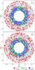 |
Fig. 2 Schematic representation of the simulated Laue lens. a) Code initialized with only Ge (111) crystals. b) Code initialized with a random crystal disposition. |
Initial parameters of the simulated Laue lens.
At this stage, the code calculated the number of crystals through Eq. (10) and the angular spread of the samples through Eq. (11). This latter is 56.72 arcsec.
The code was cycled until the system attained thermalization. To verify that the final arrangement was not affected by the initial guess and to control possible interferences of local maxima in the quantifier of Eq. (16), the algorithm was initialized with two different dispositions of the tiles. First, it was initialized with only Ge (111) CDP crystals, then with random crystals, chosen among the crystals selected at the beginning. In Fig. 2 we show the final arrangements of the crystals for the two cases, while Fig. 3 shows the effective area of the simulated Laue lens for the two cases. Finally, Table 2 lists the crystal disposition.
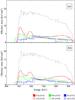 |
Fig. 3 Effective area per unit energy of the lens. The contributions of the tiles of different species are visible. Tiles were positioned in the lens to maximize the effective area in the energy range 500−850 keV and make the profile as smooth as possible with respect to energy variation. The dashed line is the total effective area. a) Code initialized with only Ge (111) crystals. b) Code initialized with a random crystal disposition. |
Crystals composing the simulated Laue lens.
After the two tests, Figs. 3 and 2 highlight an equivalent arrangement of the crystal tiles. Although the number of crystals per type and per ring are not exactly the same, very similar effective areas have been obtained, which were smooth and high for both cases. In Fig. 4 we show the photon distribution on the focal plane. The concentration of photons is high at the center of the spot and rapidly decreases farther from the center.
 |
Fig. 4 Photon distribution in the focal plane of the lens in arbitrary units. The concentration of photons is high in the focal point and rapidly decreases far from the center. The distribution is obtained with a Monte Carlo simulation. The bin width is 1 mm. |
Other examples of the use of LaueGen can be found in Bellucci et al. (2013) and Camattari et al. (2014b), who used the code to design very large Laue lenses, entirely based on quasi-mosaic crystals.
5. Conclusions
The LaueGen code has been implemented for the design of optimized Laue lenses. The program is based on a genetic algorithm. It can take into account any type of diffracting crystals and combine them to obtain the best results in terms of integrated reflectivity. In particular, the user can decide whether to prefer a lens with a high effective area or a smooth spectral response of the diffracted photons. Moreover, we showed that the final configuration of the crystals in the lens does not depend on the initial guess of initialization, that is, the global maximum can be attained by the code.
The code LaueGen can also manage the minimum distance between two neighboring samples to allow for mechanical tolerances in their assembly on the lens frame. The tolerance on crystal positioning and quality has not been implemented, but it could be easily included by introducing a random offset in the crystal position on the Laue lens and an attenuation coefficient in the theoretical reflectivity.
Since the lenses designed by the code LaueGen are not cylindrically symmetric, the photon distribution and the effective area for a source off-axis may depend on the source azimuthal position. However, this dependence is very weak because the crystals are small with respect to the lens size.
LaueGen can generate lens configurations for very different applications, from astrophysical to medical purposes. Depending on the selected degrees of freedom needed to generate a Laue lens, the code can take from tens of minutes to a few hours to run. The code has been proven to work with an example shown in this paper and with another two examples reported in the literature (Bellucci et al. 2013; Camattari et al. 2014b). The code can be a valuable tool for designing future experiments based on Laue lenses.
Acknowledgments
The authors are thankful to INFN for financial support through the LOGOS project.
References
- Authier, A. 2001, Dynamical theory of X-ray diffraction (Oxford University Press) [Google Scholar]
- Barrière, N., Ballmoos, P., Halloin, H., et al. 2006, in Focusing Telescopes in Nuclear Astrophysics, ed. P. Von Ballmoos, 269 [Google Scholar]
- Barrière, N.,Rousselle, J., von Ballmoos, P., et al. 2009, J. App. Cryst., 42, 834 [CrossRef] [Google Scholar]
- Bellucci, V.,Camattari, R., &Guidi, V. 2013, A&A, 560, A58 [Google Scholar]
- Brejnholt, N. F.,Soufli, R.,Descalle, M., et al. 2014, Opt. Express, 22, 15364 [NASA ADS] [CrossRef] [Google Scholar]
- Camattari, R.,Guidi, V.,Bellucci, V.,Neri, I., &Jentschel, M. 2013, Rev. Sci. Instrum., 84, 053110 [Google Scholar]
- Camattari, R.,Paternò, G.,Battelli, A., et al. 2014a, J. Appl. Cryst., 47, 799 [CrossRef] [Google Scholar]
- Camattari, R., Battelli, A., Bellucci, V., & Guidi, V. 2014b, Exp. Astron., in press [Google Scholar]
- Fernández-Perea, M.,Descalle, M.-A.,Soufli, R., et al. 2013, Phys. Rev. Lett., 111, 027404 [NASA ADS] [CrossRef] [Google Scholar]
- Frontera, F.,Virgilli, E.,Liccardo, V., et al. 2012, Space Telescopes and Instrumentation 2012: Ultraviolet to Gamma Ray, Proc. SPIE, 8443, 84430 [CrossRef] [Google Scholar]
- Guidi, V.,Bellucci, V.,Camattari, R., &Neri, I. 2011, J. Appl. Cryst., 44, 1255 [CrossRef] [Google Scholar]
- Keitel, S.,Malgrange, C.,Niemöller, T., &Schneider, J. R. 1999, Acta Crystallogr. A, 55, 855 [CrossRef] [Google Scholar]
- Lindquist, T. R., &Webber, W. R. 1968, Can. J. Phys., 46, S1103 [CrossRef] [Google Scholar]
- Lund, N. 1992, Exp. Astron., 2, 259 [NASA ADS] [CrossRef] [Google Scholar]
- Madsen, K. K.,Harrison, F. A.,Mao, P. H., et al. 2009, Proc. SPIE, 7437, 743716 [CrossRef] [Google Scholar]
- Malgrange, C. 2002, Cryst. Res. Tech., 37, 654 [CrossRef] [Google Scholar]
- Pisa, A. 2004, Ph.D. Thesis, Università degli Studi di Ferrara [Google Scholar]
- Roa, D.,Smither, R.,Zhang, X., et al. 2005, Exp. Astron., 20, 229 [NASA ADS] [CrossRef] [Google Scholar]
- Schonfelder, V.,Diehl, R.,Lichti, G., et al. 1984, Nuclear Science, IEEE Trans., 31, 766 [NASA ADS] [Google Scholar]
- Smither, R. K.,Saleem, K. A.,Roa, D. E., et al. 2005, Exp. Astron., 20, 201 [NASA ADS] [CrossRef] [Google Scholar]
- Sumbaev, O. 1968, Sov. Phys. JETP, 5, 724 [NASA ADS] [Google Scholar]
- Ubertini, P.,Lebrun, F., Di Cocco, G., et al. 2003, A&A, 411, L131 [NASA ADS] [CrossRef] [EDP Sciences] [Google Scholar]
- Virgilli, E.,Frontera, F.,Valsan, V., et al. 2013, Proc. SPIE, 8861, 886107 [CrossRef] [Google Scholar]
- Von Ballmoos, P., Güdel, M., Kahn, S. M., & Sunjaev, R. 2005a, High energy spectroscopic astrophysics (Springer) [Google Scholar]
- von Ballmoos, P.,Halloin, H.,Evrad, J., et al. 2005b, Exp. Astron., 20, 253 [NASA ADS] [CrossRef] [Google Scholar]
- von Ballmoos, P.,Takahashi, T., &Boggs, S. E. 2010, Nucl. Instrum. Meth. A, 623, 431 [NASA ADS] [CrossRef] [Google Scholar]
- Zachariasen, W. H. 1945, Theory of X-ray diffraction in crystals (J. Wiley and Sons, Inc.) [Google Scholar]
All Tables
All Figures
|
Fig. 1 Schematic representation of a Laue lens. The red arrows represent an X-ray beam that is diffracted toward a detector placed on the focal point of the lens. |
| In the text | |
|
Fig. 2 Schematic representation of the simulated Laue lens. a) Code initialized with only Ge (111) crystals. b) Code initialized with a random crystal disposition. |
| In the text | |
|
Fig. 3 Effective area per unit energy of the lens. The contributions of the tiles of different species are visible. Tiles were positioned in the lens to maximize the effective area in the energy range 500−850 keV and make the profile as smooth as possible with respect to energy variation. The dashed line is the total effective area. a) Code initialized with only Ge (111) crystals. b) Code initialized with a random crystal disposition. |
| In the text | |
|
Fig. 4 Photon distribution in the focal plane of the lens in arbitrary units. The concentration of photons is high in the focal point and rapidly decreases far from the center. The distribution is obtained with a Monte Carlo simulation. The bin width is 1 mm. |
| In the text | |
Current usage metrics show cumulative count of Article Views (full-text article views including HTML views, PDF and ePub downloads, according to the available data) and Abstracts Views on Vision4Press platform.
Data correspond to usage on the plateform after 2015. The current usage metrics is available 48-96 hours after online publication and is updated daily on week days.
Initial download of the metrics may take a while.