| Issue |
A&A
Volume 570, October 2014
|
|
|---|---|---|
| Article Number | A121 | |
| Number of page(s) | 13 | |
| Section | Interstellar and circumstellar matter | |
| DOI | https://doi.org/10.1051/0004-6361/201424054 | |
| Published online | 30 October 2014 | |
A Herschel [C II] Galactic plane survey
III. [C II] as a tracer of star formation
Jet Propulsion Laboratory, California Institute of Technology,
4800 Oak Grove Drive,
Pasadena,
CA
91109-8099,
USA
e-mail:
Jorge.Pineda@jpl.nasa.gov
Received: 23 April 2014
Accepted: 27 August 2014
Context. The [C ii] 158 μm line is the brightest far-infrared cooling line in galaxies, representing 0.1 to 1% of their far-infrared continuum emission, and is therefore a potentially powerful tracer of star formation activity. The [C ii] line traces different phases of the interstellar medium (ISM), including the diffuse ionized medium, warm and cold atomic clouds, clouds in transition from atomic to molecular, and dense and warm photon dominated regions (PDRs). Therefore without being able to separate the contributions to the [C ii] emission, the relationship of this fine structure line emission to star formation has been unclear.
Aims. We study the relationship between the [C ii] emission and the star formation rate (SFR) in the Galactic plane and separate the relationship of different ISM phases to the SFR. We compare these relationships to those in external galaxies and local clouds, allowing examinations of these relationships over a wide range of physical scales.
Methods. We compare the distribution of the [C ii] emission, with its different contributing ISM phases, as a function of Galactocentric distance with the SFR derived from radio continuum observations. We also compare the SFR with the surface density distribution of atomic and molecular gas, including the CO-dark H2 component.
Results. The [C ii] and SFR are well correlated at Galactic scales with a relationship that is in general agreement with that found for external galaxies. By combining [C ii] and SFR data points in the Galactic plane with those in external galaxies and nearby star forming regions, we find that a single scaling relationship between the [C ii] luminosity and SFR applies over six orders of magnitude. The [C ii] emission from different ISM phases are each correlated with the SFR, but only the combined emission shows a slope that is consistent with extragalactic observations. These ISM components have roughly comparable contributions to the Galactic [C ii] luminosity: dense PDRs (30%), cold H i (25%), CO-dark H2 (25%), and ionized gas (20%). The SFR–gas surface density relationship shows a steeper slope compared to that observed in galaxies, but one that it is consistent with those seen in nearby clouds. The different slope is a result of the use of a constant CO-to-H2 conversion factor in the extragalactic studies, which in turn is related to the assumption of constant metallicity in galaxies. We find a linear correlation between the SFR surface density and that of the dense molecular gas.
Key words: galaxies: star formation / galaxies: ISM / galaxies: evolution
© ESO, 2014
1. Introduction
The [C ii] 158 μm line is the strongest far-infrared (FIR) spectral line in galaxies, representing 0.1 to 1% of their FIR continuum emission (Stacey et al. 1991; Genzel & Cesarsky 2000). The [C ii] line is an important ISM coolant and thus has been suggested to be a powerful indicator of the star formation activity in galaxies (e.g. Boselli et al. 2002; Stacey et al. 2010; de Looze et al. 2011; Sargsyan et al. 2012, 2014; De Looze et al. 2014). Ionized carbon1 is present in a variety of phases of the interstellar medium (ISM), including the diffuse ionized medium, warm and cold atomic clouds, clouds making a transition from atomic to molecular form, and dense and warm photon dominated regions (e.g. Pineda et al. 2013). Since the [C ii] line intensity is very sensitive to the physical conditions of the line-emitting gas, and as it is produced by gas that is not directly involved in the process of star formation, the origin of its correlation with the star formation activity is uncertain. This relationship can also be affected by different environmental conditions and may vary depending on the spatial scales at which it is studied.
In most extragalactic sources studied to date [C ii] is correlated with measurements of the star formation rate (SFR). However, in some external galaxies, such as the ultra luminous infrared galaxies (ULIRGs), observations suggest a deficit of [C ii] emission with respect to the FIR emission (used to trace the SFR; e.g. Malhotra et al. 1997; Luhman et al. 1998). This deficit, however, applies only to the extreme environments of their central regions, while their disks show a relationship between [C ii] and FIR emission that is similar to that observed in normal galaxies (Díaz-Santos et al. 2014). Additionally, ULIRGS represent a small fraction of the total population of galaxies in the Universe, and therefore the potential error in the determination of the SFR from [C ii] in large samples of galaxies even including ULIRGs should be small.
The [C ii] line is a potentially important tool for tracing star formation activity as well as the physical conditions of distant galaxies. As it is a spectral line, it can be used to determine the redshift and, if the line is resolved, to determine the dynamical mass of galaxies. Additionally, as mentioned above, the [C ii] line is sensitive to the density and temperature of the line-emitting gas, and therefore can be used as a diagnostic of physical conditions. For these reasons, redshifted [C ii] will be observed in a large sample of galaxies with ALMA. Studies at small spatial scales in the local Universe are important for understanding how and why this line traces star formation and how it can be used to determine the physical conditions of the gas. Such studies are an important input for the interpretation of the observations of [C ii] in high-redshift galaxies.
To understand the relationship between the [C ii] emission and star formation in external galaxies we need to establish their relationship in our Galaxy. However, our location within the Milky Way requires that we use spectrally resolved [C ii] to locate the source of the emission as a function of radius (or position). To date the only velocity resolved Galactic survey of [C ii] is the Galactic Observations of Terahertz C+ (GOT C+) survey taken with HIFI (de Graauw et al. 2010) on Herschel (Pilbratt et al. 2010). In Pineda et al. (2013), we used the GOT C+ survey to study the distribution of the [C ii] line as a function of Galactocentric distance in the plane of the Milky Way. We used the [C ii] emission, together with that of H i, 12CO, and 13CO to study the distribution of the different phases of the interstellar medium in the plane of the Milky Way. In the present paper we compare the distribution of the [C ii] emission, as well as that of the different phases of the ISM, with that of the SFR over a wide range of physical conditions in the plane of the Milky Way. By studying the Galactic plane, we aim to provide a connection between processes in individual star forming regions and those of entire galaxies.
The determination of the SFR in the Milky Way is complicated because the far-ultraviolet (FUV) or Hα observations traditionally used in external galaxies to measure the rate are highly extinguished by the interstellar dust in the Galactic plane. Instead, several other methods are used, including observations of radio free-free (bremsstrahlung) emission (Mezger 1978; Guesten & Mezger 1982; Murray & Rahman 2010), supernova remnants (Reed 2005), pulsar counts (Lyne et al. 1985), and dust continuum emission (Misiriotis et al. 2006). When using the same initial mass function (IMF) and models of massive stars, these different methods agree that the total SFR of the Galaxy is 1.9M⊙ yr-1 (Chomiuk & Povich 2011). In this paper we use radio continuum data to determine the radial distribution of the number of Lyman continuum photons (proportional to the SFR) that best reproduces the observed free-free emission in the Galactic plane. We will then use the radial distribution of the number of Lyman continuum photons to calculate the SFR as a function of radius and compare it with the [C ii] radial emission profile.
The relationship between the star-formation activity and the gas content in galaxies has been widely studied in recent decades. It has been found that the SFR per unit area and the gas surface density in galaxies are strongly correlated (Schmidt 1959; Kennicutt 1998). This correlation suggests that how molecular clouds form out of atomic gas and how they evolve to form dense cores, which are the sites where stars form, are fundamental processes governing the evolution of galaxies. Kennicutt (1998) compared the SFR and gas (H+2H2) surface densities of a large sample of galaxies, deriving a scaling relation characterized by a power law index of 1.4. Later studies have shown that the SFR is better correlated with the surface density of H2 rather than that of H (Wong & Blitz 2002; Bigiel et al. 2008, 2011; Schruba et al. 2011). Bigiel et al. (2008) found a linear scaling relation between the SFR and H2 surface density. Similarly, Gao & Solomon (2004) used emission from HCN as a tracer of dense gas in galaxies and also found a linear scaling relation with the IR luminosity and SFR. In nearby clouds (<1 kpc from the Sun), the relationship between gas content and star formation can be accurately studied, where the gas surface density is derived using dust extinction, and the SFR is derived by counting young stellar objects (YSOs; Heiderman et al. 2010; Lada et al. 2010; Gutermuth et al. 2011). These studies suggest a steeper slope, ~2, of the SFR–gas relationship, compared with extragalactic observations. But, above a certain surface density threshold, the relationship becomes linear, suggesting that the difference between the local and extragalactic SFR–gas relationships is produced by the different fractions of dense gas traced by the observations.
Most studies of external galaxies rely on a constant CO-to-H2 conversion factor to convert the bright but optically thick 12CO J = 1 → 0 line into a H2 surface density. In Pineda et al. (2013), we used [C ii], H i, 12CO, and 13CO observations to study the surface density distribution of the different phases of the ISM, including warm and cold atomic gas, CO-dark H2, and CO-traced H2, across the Galactic plane in a detail that currently is not possible for external galaxies. We showed that the XCO conversion factor varies with Galactocentric distance as a consequence of the Galactic metallicity gradient. Additionally, we determined the distribution of the CO-dark H2 component (molecular gas that is not traced by CO but by [C ii]; Madden et al. 1997, 2013; Langer et al. 2010, 2014b; Wolfire et al. 2010), which due to the lack of [C ii] maps has only been studied in a handful of nearby galaxies (e.g. Madden et al. 1997; Cormier et al. 2014). In the present paper we analyze how the different phases of the ISM studied in Pineda et al. (2013) are related to the SFR in the Galactic plane, with the aim to reconcile the local and extragalactic SFR–gas relationships.
This paper is organized as follows. In Sect. 2, we use the observed free-free emission as a function of Galactic longitude for b = 0° to determine the distribution of the SFR in the Galaxy, and in Sect. 3 we determine the [C ii] luminosity distribution of the Milky Way based on the azimuthally averaged [C ii] emissivities derived in Pineda et al. (2013) and the scale height of the [C ii] emission derived by Langer et al. (2014a). In Sect. 4 we compare the SFR of the Galaxy with the [C ii] emission arising from the different ISM phases. In Sect. 5, we study the relationship between the SFR and the gas content of these ISM phases, and in Sect. 6, we summarize our results.
2. Star formation rate distribution
The thermal radio continuum (free-free) emission arising from ionized gas can be used to determine the number of Lyman continuum (Lyc) photons, NLyc, produced by ionizing stars. NLyc can then be used to determine the SFR required to maintain a steady-state population of these stars. It has been shown that most O stars in the Galaxy are located in (and ionize) extended low density H ii regions (Mezger 1978), with only 10–20% of O stars being embedded in compact H ii regions (Mezger & Smith 1976). The extended free-free emission observed in the Galactic plane originates mostly from an ensemble of evolved H ii regions whose Strömgren spheres partially overlap. In the following, we refer to this component of the ionized gas as the extended low density warm ionized medium (ELDWIM).
We used the 1.4 GHz free-free intensity distribution as a function of Galactic longitude (l), and latitude (b = 0°), Iff(l,b = 0°), to derive the radial distribution of the SFR in the Galactic plane. The free-free intensities are taken from Guesten & Mezger (1982) and were derived by Mathewson et al. (1962) and Westerhout (1958) for the southern and northern parts of the Galaxy, respectively. The frequency and angular resolution of these data sets are (1.44 GHz, 50′) for the Mathewson et al. (1962) and (1.39 GHz, 34′) for the Westerhout (1958) data sets2. To isolate the contribution from free-free emission in the observed radio continuum distribution, Westerhout (1958) and Mathewson et al. (1962) subtracted the contribution from non-thermal synchrotron emission using the 85.5 MHz survey by Hill et al. (1958) (which is dominated by non-thermal emission) assuming a flux density spectral index (I ∝ νβ) for this emission mechanism of β = −2.6, between 85.5 MHz and 1.4 GHz. The uncertainties in the assumed spectral index of the non-thermal emission dominates the uncertainties in the separation between thermal and non-thermal contributions to the 1.4 GHz emission. To compare the free-free distribution from Westerhout (1958) and Mathewson et al. (1962) with modern-day data, we compared it with that derived for WMAP by Gold et al. (2011) at 23 GHz using the Maximum Entropy Method with 1° angular resolution. This data set includes the extended free-free emission originating from the ELDWIM plus that from compact H ii regions. We corrected for the difference in frequencies between the two data sets and reduced the emission derived for WMAP by 50% as suggested by Alves et al. (2012). We find that the longitudinal distribution of the ELDWIM free-free emission derived for WMAP and those derived by Westerhout (1958) and Mathewson et al. (1962) are in good agreement, with their intensities agreeing within 20–30%. We assumed uncertainties in the free-free distribution of 30%. Note that we prefer to use the free-free distribution from Westerhout (1958) and Mathewson et al. (1962) because point sources have been subtracted (by identifying closed contours in their maps having sizes close to that of their beam size), and therefore their data set corresponds to the free-free emission originating from the ELDWIM. The contribution from compact H ii in the derivation of the SFR will be added in later in our analysis. We first converted the free-free intensity to the radial distribution of the azimuthally averaged free-free emissivity. This emissivity can be converted into the radial distribution of the SFR as described below.
We assumed that the galaxy is axisymmetric and can be divided in a set of Nrings concentric rings of radius Ri with each having an azimuthally-averaged free-free emissivity ϵff(Ri). The free-free intensity for a given line-of-sight defined by its Galactic longitude lj is a linear sum over all rings that it intersects,  (1)where Lij describes the path length subtended over a Galactocentric ring Ri by a line-of-sight with Galactic longitude lj and MLOS is the number of sampled lines of sight. (For an illustration of the adopted geometry see Fig. A.1 in Pineda et al. 2013.) This set of MLOS × Nrings linear equations can in principle be inverted in the case where the number of samples of the free-free intensity (MLOS) is equal to the number of Galactocentric rings that produce the emission (Nrings), resulting in the distribution of ϵff(R) that reproduces the distribution of Iff(l). In practice, however, we do not expect to have an exact solution because the Galaxy is not axisymmetric and the number of rings typically available is not large enough to sample properly the Iff(l) distribution. We instead search for the distribution ϵff(R) that minimizes the χ2 calculated between the observed Iff(l) distribution and that resulting from a modeled ϵff(R) distribution. Because the contribution from outer galaxy rings to the free-free brightness temperature is likely to be very small, there could be solutions that will have an oscillatory behavior in the outer galaxy and still produce an integrated intensity along the line of sight that is close to zero. Additionally, rings close to the Galactic center are not well sampled by the Iff(l) distribution. Therefore, following Assef et al. (2008, 2010), we include a smoothing term H in the minimization that forces rings near the Galactic Center (Rgal< 3 kpc) and in the outer galaxy (Rgal> 8.5 kpc) to be close to zero. We tested the effect of varying these limits in Rgal in the solution of the χ2 minimization and found that while the solution does not vary significantly for 3 kpc <Rgal< 8.5 kpc, using the smoothing term does minimize the oscillatory behavior for the solution outside this range in Galactocentric distance. We therefore minimize the function
  (2)where η is a free parameter that can be adjusted to keep the values near the Galactic center and in the outer galaxy close to zero. The χ2 function is given by
 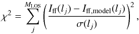 (3)where σ(lj) are the uncertainties in the free-free intensity and Iff,model(lj) is the free-free intensity predicted at lj for a given radial emissivity distribution. The smoothing term is given by
  (4)where Ri0 = 3 kpc and Ri1 = 8.5 kpc define the range in Galactocentric distance in which we expect to have most of the contribution to the observed free-free intensity. Minimizing the function G results in the set of equations
 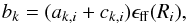 (5)where
 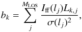 (6)
(6) (7)and
 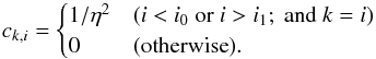 (8)This set of MLOS × MLOS equations can be written in vector-matrix form as
 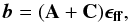 (9)and the radial distribution of the free-free emissivity that best reproduced the observed Iff(l) distribution can be determined by inverting the A + C matrix. The Iff(l) distribution used in our calculation is the average between that derived for the northern and southern parts of the Galaxy. Note that because all parameters involved in our calculation are linear, the solution we found by inverting the A + C matrix corresponds to the global minimum of the function G (Eq. (2)). In the upper panel of Fig. 1, we show the resulting distribution of the free-free emissivity as a function of Galactocentric distance. The uncertainties in the emissivity distribution are given by the square root of the diagonal terms in the (A + C)-1 matrix. The resulting free-free emissivity distribution is in good agreement with that derived by Guesten & Mezger (1982), which employed the same free-free data set but a different technique to determine the SFR.
 |
Fig. 1 Upper panel: radial distribution of the free-free emissivity resulting from the average of those from the north and south portions of the Galaxy for Rgal> 2 kpc. Lower panel : radial distribution of the SFR derived following the method described in Sect. 2 for Rgal> 2 kpc. |
The free-free luminosity is related to the flux density observed at a distance D as,  (10)where Sff is the flux density of the ring, which for D ≫ Rgal, is given by,
  (11)Here, Iff(Rgal) is the free-free continuum intensity at the surface of a ring centered at a Galactocentric distance Rgal. We assumed that the vertical distribution of the free-free emissivity is Gaussian with a peak emissivity given by that at b = 0° and a FWHM Δzff of 260 pc (Mezger 1978). Note that pulsar dispersion observations suggest the existence of a lower density ionized gas component that extends even further vertically than the ELDWIM (Δz = 1 kpc; Kulkarni & Heiles 1987; Reynolds 1989). Iff(Rgal) is related to the azimuthally averaged free-free emissivity at b = 0°, ϵff(Rgal), as
  (12)The free-free luminosity for a ring is therefore given by
  (13)We use the free-free luminosity distribution to calculate the number of Lyc photons per second absorbed by the gas at Galactocentric distance Rgal. The number of Lyc photons absorbed per second by the ionized gas with electron temperature Te and at distance D, which emits free-free luminosity Lff is given by Mezger (1978)
![\begin{eqnarray} \label{eq:1} \left[\frac{N_{\rm Lyc}(R_{\rm gal})}{\rm photons\,s^{-1}}\right]= \,\frac{1.25}{(1+y^+)}6.32\times10^{52}\!\left[\frac{T_{\rm e}}{\rm 10^4 \,K} \right]^{-0.45}\!\left[\frac{\nu}{\rm GHz} \right]^{0.1}\!\left[\frac{L_{\rm ff}(R_{\rm gal})}{\rm 10^{27}\, erg\,s^{-1}\,Hz^{-1}} \right], \end{eqnarray}](/articles/aa/full_html/2014/10/aa24054-14/aa24054-14-eq71.png) (14)where y+ = 0.08 corrects for the abundance of singly ionized He and the factor 1.25 accounts for the number of Lyc photons directly absorbed by dust (we assumed that the number of Lyc photons that can escape the Galactic disk is negligible). We assumed an electron temperature, Te = 7000 K (Mezger 1978). We also include in the radial distribution of the number of Lyc photons the contribution from Lyc photons ionizing compact H ii regions (Smith et al. 1978). This contribution is small compared with that from the ELDWIM (Mezger 1978), but it extends over a wider range of Galactocentric distances.
(14)where y+ = 0.08 corrects for the abundance of singly ionized He and the factor 1.25 accounts for the number of Lyc photons directly absorbed by dust (we assumed that the number of Lyc photons that can escape the Galactic disk is negligible). We assumed an electron temperature, Te = 7000 K (Mezger 1978). We also include in the radial distribution of the number of Lyc photons the contribution from Lyc photons ionizing compact H ii regions (Smith et al. 1978). This contribution is small compared with that from the ELDWIM (Mezger 1978), but it extends over a wider range of Galactocentric distances.
The SFR required to maintain a steady-state population of ionizing stars that produces the observed number of Lyman continuum photons per second can be determined using the relationship SFR[M⊙ yr-1 ] = 7.5 × 10-54NLyc [ photons s-1 ] estimated by Chomiuk & Povich (2011) assuming a Kroupa IMF (Kroupa & Weidner 2003), Solar metallicity, and considering population models of O stars. The resulting radial distribution of the SFR in the Galactic plane for Rgal> 2 kpc is shown in the lower panel of Fig. 1. Integrating the SFR across the galaxy, we obtain a total SFR for the Milky Way of 1.8 ± 0.1 M⊙ yr-1, in excellent agreement with the 1.9 ± 0.4 M⊙ yr-1 estimated by Chomiuk & Povich (2011) using several independent methods. Note that our estimation of the total SFR of the Milky Way does not include the contribution from the Galactic center. The uncertainties in our estimation the Galactic SFR are likely a lower limit, as these are calculated by propagating the errors of the radial SFR distribution shown in Fig. 1, and do not account for uncertainties resulting from the conversion from NLyc to SFR and the assumption that the Galaxy is axisymmetric. Guesten & Mezger (1982) studied the effect on the radial distribution of NLyc of considering the spiral arm structure of the Milky Way, which is a barred spiral (SBc) galaxy. They show that within the accuracy of their estimation of NLyc(Rgal), accounting for spiral arms does not have a significant effect on the derived contribution compared to that derived under the assumption of azimuthal symmetry.
The free-free emission originates from H ii regions that are produced by massive stars (M> 15 M⊙), and therefore traces the star formation averaged over 3–10 Myr, which is the lifetime of O stars (e.g. Kennicutt & Evans 2012). On the other hand, the FUV that heats the neutral ISM, which is later cooled by [C ii], also originates from B-stars with masses above 5 M⊙ (Parravano et al. 2003), thus tracing the SFR over a longer time scale (100 Myr). Note that the conversion between NLyc and the SFR needs to be evaluated over spatial scales that are sufficiently large that the IMF is well sampled (see e.g. Vutisalchavakul & Evans 2013). By dividing the Milky Way in a set of rings, we are averaging free-free continuum emission, and therefore evaluating the SFR, over scales between 10 to 30 kpc2, which correspond to the range of the ring areas considered here. For such areas, the IMF is expected to be fully sampled (Kennicutt & Evans 2012). Another assumption that we need to make to use the Lyc continuum photons to trace the SFR is a continuous star formation over the scales at which this SFR calibration works (3–10 Myr). This assumption is justified as the SFR in the Milky Way has been suggested to be nearly continuous over the last ~8 Gyr (Noh & Scalo 1990; Rocha-Pinto et al. 2000; Fuchs et al. 2009) with some variation on a period of ~400 Myr (Rocha-Pinto et al. 2000), thus the timescales for variation in the SFR are much longer than that on which the Lyc photons trace the SFR.
Note that the conversion from the number of Lyc photons to the SFR is sensitive to metallicity, which is known to vary with Galactocentric distance (e.g Rolleston et al. 2000). These effects have been studied with evolutionary synthesis models by Schaerer & Vacca (1998) and Smith et al. (2002) (see also Kennicutt & Evans 2012). According to the models of Smith et al. (2002), for continuous star formation at a rate of 1 M⊙ yr-1, the resulting ionizing photon luminosity varies by only 30% for a factor of 5 change in metallicity. In the range where most of the free-free emissivity is observed in the Galactic plane, 3 kpc <Rgal< 10 kpc, the metallicity varies by a factor of 1.5 from its average value (1.5 Z⊙), for the metallicity gradient fitted by Rolleston et al. (2000). We therefore expect that the dependence of the conversion from NLyc and SFR with metallicity is negligible in the Galactic plane, and we use the conversion for solar metallicity without any further correction.
3. [C II] luminosity of the Milky Way
We estimated the radial luminosity distribution of the different ISM components contributing to the observed [C ii] emissivity in the Galactic plane (dense photon dominated regions, hereafter PDRs, cold H i, CO-dark H2, and ionized gas). We determined the [C ii] luminosity distributions using the emissivity distributions derived in Pineda et al. (2013) following the same procedure used to determine the free-free luminosity, ![\begin{equation} L_{\rm [CII]}(R_{\rm gal})= \frac{2(2\pi)^{5/2}}{2.354} \epsilon_{\rm [CII]}(R_{\rm gal})\Delta z_{\rm [CII]} \Delta R_{\rm gal} R_{\rm gal}. \end{equation}](/articles/aa/full_html/2014/10/aa24054-14/aa24054-14-eq84.png) (15)Following the results presented by Langer et al. (2014a), we assume a scale height of the Galactic disk with a FWHM of 172 pc for the CO-dark H2 gas, 212 pc for the cold H i gas (Dickey & Lockman 1990), and 130 pc for the dense PDR component. We considered the diffuse ionized component discussed by Kulkarni & Heiles (1987) and Reynolds (1989), that has a FWHM of 1 kpc. This scale height is consistent with that constrained by pulsar dispersion in the NE2001 model (Cordes & Lazio 2003). The resulting [C ii] luminosity distributions are shown in Fig. 2. We also show the radial distribution of the total [C ii] luminosity of the Milky Way, which is the sum of the luminosity from all contributing ISM components. The total [C ii] luminosity of the Milky Way and the contributions to that from different ISM components are listed in Table 1. The [C ii] luminosity of the different ISM components is the sum of that for each Galactocentric ring,
(15)Following the results presented by Langer et al. (2014a), we assume a scale height of the Galactic disk with a FWHM of 172 pc for the CO-dark H2 gas, 212 pc for the cold H i gas (Dickey & Lockman 1990), and 130 pc for the dense PDR component. We considered the diffuse ionized component discussed by Kulkarni & Heiles (1987) and Reynolds (1989), that has a FWHM of 1 kpc. This scale height is consistent with that constrained by pulsar dispersion in the NE2001 model (Cordes & Lazio 2003). The resulting [C ii] luminosity distributions are shown in Fig. 2. We also show the radial distribution of the total [C ii] luminosity of the Milky Way, which is the sum of the luminosity from all contributing ISM components. The total [C ii] luminosity of the Milky Way and the contributions to that from different ISM components are listed in Table 1. The [C ii] luminosity of the different ISM components is the sum of that for each Galactocentric ring, ![\begin{equation} L_{\rm [CII]}=\sum^{N}_{i} L_{\rm [CII]}(R^i_{\rm gal}). \end{equation}](/articles/aa/full_html/2014/10/aa24054-14/aa24054-14-eq85.png) (16)The ISM components that contribute to the [C ii] luminosity of the Milky Way have roughly comparable contributions: dense PDRs (30%), cold H i (25%), CO-dark H2 (25%), and ionized gas (20%).
(16)The ISM components that contribute to the [C ii] luminosity of the Milky Way have roughly comparable contributions: dense PDRs (30%), cold H i (25%), CO-dark H2 (25%), and ionized gas (20%).
Note that the contribution from ionized gas to the total [C ii] luminosity of the Galaxy is much larger than its ~4% contribution to the total [C ii] emissivity at b = 0° estimated by Pineda et al. (2013), using the NE2001 (Cordes & Lazio 2002) model of the distribution of ionized gas in the Galaxy. The [C ii] emission associated with ionized gas is expected to be diffuse but much more vertically extended compared with the other [C ii]-emitting ISM components. Therefore, since the scale height of the ionized gas is much larger than that of either atomic and molecular gas, the [C ii] luminosity associated with ionized gas becomes significant despite its emissivity at b = 0° being relatively low. The larger contribution of ionized gas to the total [C ii] luminosity of the Milky Way is in agreement with the suggestion by Heiles (1994), that ionized gas could be a significant contributor to the [C ii] intensity observed by COBE. Note that the NE2001 model assumes a distribution of electron densities that is smooth on the order of kpc scales. Therefore, our estimate of the contribution of the ionized gas to the total [C ii] luminosity should be considered as a lower limit, in the case that the ELDWIM is clumpy.
 |
Fig. 2 The [C ii] luminosity of the Milky Way as a function of Galactocentric radius. The estimated contributions to the [C ii] luminosity from gas associated with dense PDRs, ionized gas, CNM H i gas, and CO-dark H2 gas are also shown. Typical uncertainties are 5% for the total [C ii] luminosity and the contribution from H i gas, 10% for the contribution from CO-dark H2 gas, and we assume 30% for the contribution from ionized gas. The black dots (and error bars) represent the radial distribution of the SFR derived in Sect. 2. |
 |
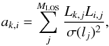
Fig. 3 Upper panel: comparison between the SFR and the observed [C ii] luminosity for different rings in the Milky Way. The dashed straight line represents a fit to the data while the solid straight line is the relationship between the SFR and [C ii] luminosity fitted by de Looze et al. (2011) for a set of nearby galaxies. Lower panel: comparison between the SFR surface density and the [C ii] luminosity per unit area. The dashed straight line represents a fit to the data. |
We estimate a total [C ii] luminosity of the Milky Way of ![\hbox{$L^{\rm MW}_{\rm [CII]}=1.0\times10^{41}$}](/articles/aa/full_html/2014/10/aa24054-14/aa24054-14-eq86.png) erg s-1. This value of
erg s-1. This value of ![\hbox{$L^{\rm MW}_{\rm [CII]}$}](/articles/aa/full_html/2014/10/aa24054-14/aa24054-14-eq87.png) is about half that estimated by Wright et al. (1991) of
is about half that estimated by Wright et al. (1991) of ![\hbox{$L^{\rm MW}_{\rm [CII]}=1.95\times10^{41}$}](/articles/aa/full_html/2014/10/aa24054-14/aa24054-14-eq88.png) erg s-1 using COBE data. Wright et al. (1991) derived the [C ii] luminosity using
erg s-1 using COBE data. Wright et al. (1991) derived the [C ii] luminosity using ![\hbox{$L^{\rm MW}_{\rm [CII]}=4\pi R_\odot^2[(1.35$}](/articles/aa/full_html/2014/10/aa24054-14/aa24054-14-eq89.png) sr)⟨ I[ CII ] ⟩], where ⟨ I[ CII ] ⟩ = 1.7 ± 0.07 × 10⁻⁵ erg cm-2 s-1 sr-1 is the mean [C ii] intensity observed by COBE. The average [C ii] intensity is derived over a solid angle of 1.35 sr, which is the result of the integral of a source function that is derived by fitting the distribution of dust continuum emission observed by COBE. Because the spatial distribution of the dust continuum distribution is not necessarily the same as that of [C ii], this might be the origin of the discrepancy. To understand the source of the difference with COBE we analyzed the GOT C+ data using an approach similar to that used for the COBE data as follows. We constructed a synthetic map of the Milky Way in [C ii] using the radial distribution of the [C ii] emissivity shown in Fig. 4 in Pineda et al. (2013) and assuming a FWHM of the [C ii] emission of 172 pc. This map is then convolved with a 7° beam to simulate the emission observed by COBE. Since Wright et al. (1991) do not provide the functional form of the source function, we used the publicly available FIRAS data (which was reprocessed by Bennett et al. 1994) to estimate the mean [C ii] intensity observed by COBE. Integrating the [C ii] emission in the COBE map using a 5σ threshold, where σ = 7 × 10⁻⁷ erg cm-2 s-1 sr-1, yields an average [C ii] intensity ⟨ I[ CII ] ⟩ = 1.8 × 10⁻⁵ erg cm-2 s-1 sr-1, which is consistent with that published by Wright et al. (1991). In our simulated map, the 5σ limit yields an averaged intensity of ⟨ I[ CII ] ⟩ = 1.6 × 10⁻⁵ erg cm-2 s-1 sr-1, which corresponds, using the equation used by Wright et al. (1991), to
sr)⟨ I[ CII ] ⟩], where ⟨ I[ CII ] ⟩ = 1.7 ± 0.07 × 10⁻⁵ erg cm-2 s-1 sr-1 is the mean [C ii] intensity observed by COBE. The average [C ii] intensity is derived over a solid angle of 1.35 sr, which is the result of the integral of a source function that is derived by fitting the distribution of dust continuum emission observed by COBE. Because the spatial distribution of the dust continuum distribution is not necessarily the same as that of [C ii], this might be the origin of the discrepancy. To understand the source of the difference with COBE we analyzed the GOT C+ data using an approach similar to that used for the COBE data as follows. We constructed a synthetic map of the Milky Way in [C ii] using the radial distribution of the [C ii] emissivity shown in Fig. 4 in Pineda et al. (2013) and assuming a FWHM of the [C ii] emission of 172 pc. This map is then convolved with a 7° beam to simulate the emission observed by COBE. Since Wright et al. (1991) do not provide the functional form of the source function, we used the publicly available FIRAS data (which was reprocessed by Bennett et al. 1994) to estimate the mean [C ii] intensity observed by COBE. Integrating the [C ii] emission in the COBE map using a 5σ threshold, where σ = 7 × 10⁻⁷ erg cm-2 s-1 sr-1, yields an average [C ii] intensity ⟨ I[ CII ] ⟩ = 1.8 × 10⁻⁵ erg cm-2 s-1 sr-1, which is consistent with that published by Wright et al. (1991). In our simulated map, the 5σ limit yields an averaged intensity of ⟨ I[ CII ] ⟩ = 1.6 × 10⁻⁵ erg cm-2 s-1 sr-1, which corresponds, using the equation used by Wright et al. (1991), to ![\hbox{$L^{\rm MW}_{\rm [CII]}=1.8\times 10^{41}$}](/articles/aa/full_html/2014/10/aa24054-14/aa24054-14-eq98.png) erg s-1, in excellent agreement with the [C ii] luminosity suggested by COBE. Therefore the difference between the [C ii] luminosities derived from GOT C+ and COBE likely arises from the different methods and assumptions used regarding the volume distribution of [C ii] emission. Note also that there may be some uncertainty on the absolute flux calibration of the COBE/FIRAS instrument, as suggested by the discrepancy between absolute [C ii] fluxes observed by COBE/FIRAS and FILM/IRTS (Makiuti et al. 2002), with the latter instrument showing ~50% lower flux. We suggest that our [C ii] luminosity estimation is better suited for comparison with external galaxies than that presented by Wright et al. (1991).
erg s-1, in excellent agreement with the [C ii] luminosity suggested by COBE. Therefore the difference between the [C ii] luminosities derived from GOT C+ and COBE likely arises from the different methods and assumptions used regarding the volume distribution of [C ii] emission. Note also that there may be some uncertainty on the absolute flux calibration of the COBE/FIRAS instrument, as suggested by the discrepancy between absolute [C ii] fluxes observed by COBE/FIRAS and FILM/IRTS (Makiuti et al. 2002), with the latter instrument showing ~50% lower flux. We suggest that our [C ii] luminosity estimation is better suited for comparison with external galaxies than that presented by Wright et al. (1991).
4. [C II] as an indicator of the star formation rate
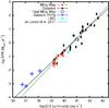 |
Fig. 4 Star formation rate as a function of [C ii] luminosity for different rings in the Galaxy, the LMC, the galaxies studied by de Looze et al. (2011), and for individual Galactic PDRs. The [C ii] luminosity of the LMC is taken from Rubin et al. (2009) and the SFR from Harris & Zaritsky (2009). The Galactic PDR data points include Orion (L[ CII ] from Stacey et al. 1993, and SFR from Lada et al. 2010), M17 (L[ CII ] from Stacey et al. 1991, and SFR from Lada et al. 2010), Rosette (L[ CII ] from Schneider et al. 1998 and SFR from Chomiuk & Povich 2011), and Carina (L[ CII ] from Brooks et al. 2003 and SFR from Chomiuk & Povich 2011). The [C ii] luminosities and SFRs for this sample are strongly correlated over 6 orders of magnitude. |
Correlation between the [C ii] luminosity of the different contributing ISM components and the SFR for different rings in the Galactic plane obtained using BES fits.
In Fig. 2, we show the radial distribution of the SFR together with that of the total [C ii] luminosity and the different contributing ISM components. The SFR and total [C ii] luminosity distributions are very similar with most of the star-formation taking place and the [C ii] emission being produced between 4 and 10 kpc. Both distributions show a peak at ~4.5 kpc from the Galactic center.
In the top panel of Fig. 3, we show the SFR as a function of the [C ii] luminosity between 4 and 10 kpc for bins in Galactocentric radius of 0.5 kpc width. As discussed in Pineda et al. (2013), we find that the bin width of 0.5 kpc over the range of Galactocentric distance used here allows us to study radial variations of the [C ii] emission while ensuring that each ring is sufficiently sampled by the GOT C+ data. The uncertainties in the [C ii] luminosity are derived by the propagation of the errors in the integrated intensities measured for all samples of a given ring (see Pineda et al. 2013). We fitted a straight line to the data using the orthogonal bi-variate error and intrinsic scatter method (BES; Akritas & Bershady 1996). The result of the fit ![\begin{equation} \log {\it SFR} = m \log L_{\rm [CII]}+b, \end{equation}](/articles/aa/full_html/2014/10/aa24054-14/aa24054-14-eq105.png) (17)where m is the slope and b the intercept, is shown in the top panel of Fig. 3 and listed in Table 1. We also include in Table 1 the standard deviation, which measures the dispersion of the observed SFRs from the fit, and the Spearman’s rank coefficient, ρ, which evaluates the strength of the correlation3. We also show the fit to the relationship between SFR and [C ii] luminosity for a sample of nearby galaxies presented by de Looze et al. (2011), who sampled 24 nearby star-forming galaxies, including starbursts and low-ionization nuclear emission-line region (LINERs) galaxies. The SFR and the total [C ii] luminosity we determined from the GOT C+ data are well correlated (ρ = 0.91), with a slope that is in very good agreement with that estimated by de Looze et al. (2011). The dispersion of the observed SFRs from the fit is 0.14 dex which is smaller than the 0.27 dex found by de Looze et al. (2011) for their sample of galaxies, which could be an indication that the variation in the ISM conditions (e.g. densities, temperatures, FUV fields) within the Milky Way is smaller than that among the galaxies in their sample. A factor that could enhance the observed correlation is the fact that both the [C ii] luminosity and SFR are functions of the area of a given ring, which is in turn a function of Galactocentric distance. In the bottom panel of Fig. 3 we show the SFR surface density (SFR/area) as a function of the [C ii] luminosity divided by area. We see that the correlation still holds, with a Spearman’s rank coefficient of 0.92, thus indicating that the ring area is not the source of the correlation seen above. The straight line fit, log (ΣSFR[M⊙ yr-1 kpc-2)] = (0.99 ± 0.06)log (L[ CII ]/ Area [erg s-1 pc-2] −(34.50 ± 1.80), also shows that the slope is very similar to that of derived for the correlation between [C ii] and SFR.
(17)where m is the slope and b the intercept, is shown in the top panel of Fig. 3 and listed in Table 1. We also include in Table 1 the standard deviation, which measures the dispersion of the observed SFRs from the fit, and the Spearman’s rank coefficient, ρ, which evaluates the strength of the correlation3. We also show the fit to the relationship between SFR and [C ii] luminosity for a sample of nearby galaxies presented by de Looze et al. (2011), who sampled 24 nearby star-forming galaxies, including starbursts and low-ionization nuclear emission-line region (LINERs) galaxies. The SFR and the total [C ii] luminosity we determined from the GOT C+ data are well correlated (ρ = 0.91), with a slope that is in very good agreement with that estimated by de Looze et al. (2011). The dispersion of the observed SFRs from the fit is 0.14 dex which is smaller than the 0.27 dex found by de Looze et al. (2011) for their sample of galaxies, which could be an indication that the variation in the ISM conditions (e.g. densities, temperatures, FUV fields) within the Milky Way is smaller than that among the galaxies in their sample. A factor that could enhance the observed correlation is the fact that both the [C ii] luminosity and SFR are functions of the area of a given ring, which is in turn a function of Galactocentric distance. In the bottom panel of Fig. 3 we show the SFR surface density (SFR/area) as a function of the [C ii] luminosity divided by area. We see that the correlation still holds, with a Spearman’s rank coefficient of 0.92, thus indicating that the ring area is not the source of the correlation seen above. The straight line fit, log (ΣSFR[M⊙ yr-1 kpc-2)] = (0.99 ± 0.06)log (L[ CII ]/ Area [erg s-1 pc-2] −(34.50 ± 1.80), also shows that the slope is very similar to that of derived for the correlation between [C ii] and SFR.
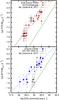 |
Fig. 5 Upper panel: comparison between the SFR and the contribution to the [C ii] luminosity from PDRs and electrons, and bottom panel: from cold H i and CO-dark H2 gas. In both panels the dashed straight lines represent fits to the data and the solid straight line is the relationship between the SFR and [C ii] luminosity fitted by de Looze et al. (2011) in a set of nearby galaxies. Typical uncertainties are 5% for the total [C ii] luminosity and the contribution from H i gas, 10% for the contribution from CO-dark H2 gas, and 30% for the contribution from ionized gas. |
In Fig. 4, we show the SFR as a function of [C ii] luminosity for rings in the Galaxy, the LMC, the Galaxies studied by de Looze et al. (2011), and Galactic PDRs. To determine the SFR in their sample of Galaxies, de Looze et al. (2011) used the FUV+24 μm emission, while the SFR of Galactic star-forming regions was determined using YSO counts (Chomiuk & Povich 2011; Lada et al. 2010). The different methods used for determining the SFR are likely one of the main reasons for the large scatter (0.3 dex) in the relationship (Vutisalchavakul & Evans 2013). Nevertheless, we see that the SFR and [C ii] luminosity are correlated (ρ = 0.98) over 6 orders of magnitude. We fitted a straight line to the combined data resulting in the relationship, log (SFR[M⊙ yr-1]) = (0.89 ± 0.04)log (L[ CII ][erg s-1 ] ) − (36.3 ± 1.5). The good correlation between the [C ii] luminosity and SFR suggests that [C ii] is a good tracer of the star formation activity in the Milky Way, as well as in nearby galaxies dominated by star formation.
We also investigated the relationship between the SFR and [C ii] luminosity emerging from the different contributing ISM components. In Fig. 5 we compare the SFR versus the [C ii] luminosity arising from dense PDRs, cold H i gas, ionized gas, and CO-dark H2 gas for bins in Galactocentric radius of 0.5 kpc. We list the results of straight line fits in Table 1, and we show the resulting fits in Fig. 5. For comparison we also include the fit for nearby galaxies by de Looze et al. (2011). The [C ii] luminosity for the different contributing components are well correlated with the SFR (ρ = 0.86−0.94) with dispersions in the 0.1–0.2 dex range. The slope of the relationships between the SFR and the [C ii] luminosity arising from PDRs and ionized gas are similar to that found for the relationship involving the total [C ii] luminosity. For the relationship involving the cold H i gas, the relationship is somewhat shallower, while for the relationship involving the CO-dark H2 gas, the slope is significantly steeper. At larger Galactocentric distances (8−10 kpc), where there is little star formation, the [C ii] luminosity associated with H i is a weak contributor, while CO-dark H2 dominates the [C ii] luminosity. The [C ii] luminosity arising from PDRs, ionized gas, and atomic gas show an steeper increase at smaller Galactocentric distances compared to that originating from the CO-dark H2 gas. This increase in the [C ii] luminosity is a result of the combined effect of an increased column density and thermal pressure. The column density of the CO-dark H2, however, stays constant between 4 and 10 kpc (Pineda et al. 2013), as the increased H2 column densities, which is associated with a greater dust shielding, enhances the abundance of CO. The constant CO-dark H2 column density results in a shallower increase in the [C ii] luminosity for reduced Galactocentric distances, which in turn results in an steeper relationship with the SFR compared with that involving the other ISM contributing components. The difference between the slopes of the different ISM contributing components to the [C ii] luminosity suggests that the observed correlation between the total L[ CII ] and SFR is the result of the combined emission of the different contributing ISM phases. Most FUV photons produced by young stars are involved in heating the gas. As the gas becomes warmer, the  level of C+ can be more readily populated by collisions, and the rate of emission of [C ii] photons is increased. Therefore, the [C ii] emission is indirectly related to the process of star formation, regardless from which ISM phase it emerges.
In thermal equilibrium, the gas heating, which is dominated by the photo-electric effect of FUV photons in dust grains and is thus proportional to the SFR, is expected to be balanced by the gas cooling, which is dominated by [C ii] emission (except in the brightest and densest PDRs, where [O i] emission also contributes, and in ionized gas regions where excitation of low lying electronic states of trace species such as O++ and N+ dominates). For Gaussian distributions of the [C ii] intensity and H column density, we can calculate the midplane cooling rate per hydrogen nucleus for a given Galactocentric radius as Λ(Rgal) = L[ CII ](Rgal) /MH(Rgal), where L[ CII ](Rgal) is the [C ii] luminosity and MH(Rgal) is the H mass of a given ring. To calculate the cooling rate, we used the luminosity distribution of the different ISM components presented in Fig. 2, and we estimated their H mass from the surface density distributions presented in Pineda et al. (2013), with the exception of the dense PDR component (see below). In the upper panel of Fig. 6 we compare the cooling rate from the different ISM components with the SFR for different Galactocentric radii. As expected, we see a good correlation between Λ and the SFR, with the different ISM components having relationships with the SFR that have similar slopes.
We can understand the slope of the relationship between the cooling rate of the different ISM components considering the distribution of Λ as a function of Galactocentric radius. In the lower panel of Fig. 6 we see that the cooling rate increases with decreasing Galactocentric radius. It can be shown that for [C ii] in the optically thin and subthermal regime, the cooling rate per H nuclei is proportional to the C+ to H abundance ratio, the collisional rate coefficient, the H volume density, and is a function of the kinetic temperature (Wiesenfeld & Goldsmith 2014; Goldsmith et al. 2012). Thus, the increase in the cooling rate for decreasing Galactocentric radius is produced by volume density and abundance gradients. This trend is exemplified by the straight lines seen for the CO-dark H2 and cold H i (CNM) components which are a reflection of the adopted thermal pressure gradient from Wolfire et al. (2003), which is used to calculate the volume density assuming a constant kinetic temperature, and the carbon abundance gradient from Rolleston et al. (2000). Both the volume density and the C+ relative abundance increase by a factor ~3 going from 10 kpc to 4 kpc. Therefore, we suggest that the slope of the relationship between the cooling rate and the SFR is a result of a combined effect of the volume density and carbon abundance gradients in the Galactic plane.
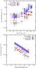 |
Fig. 6 Upper panel: the [C ii] cooling rate per H atom as a function of the SFR for line-emitting gas associated with dense PDRs, cold H i gas, CO-dark H2 gas, and ionized gas. Lower panel: the [C ii] cooling rate as a function of Galactocentric radius for the different contributing ISM phases discussed in the text. |
Note that we estimated the H mass distribution associated with dense PDRs using 12CO and 13CO observations using the method described in Pineda et al. (2013) for pixels in the position-velocity map where [C ii], 12CO, and 13CO are detected. The derived column density does not necessarily represent the column of gas associated with [C ii] emission as there might be gas that is shielded from the FUV photons where most of the carbon is in the form of CO. Therefore, we consider the derived cooling rate for dense PDRs as a lower limit. This effect should also vary as a function of Galactocentric radius, as the average gas column density (and the fraction of shielded gas) increases with Galactocentric distance (see Fig. 9). This effect might explain the flatter slope seen in the cooling rate as a function of Galactocentric distance.
5. The relationship between gas content and star-formation in the disk of the Milky Way
Starting with the work by Schmidt (1959) and Kennicutt (1998), numerous studies have focused on the relationship between the star formation activity and gas content in galaxies. The relationship between SFR and gas surface density has been evaluated over a wide range of spatial scales including entire galaxies, within resolved disks of nearby galaxies (e.g. Bigiel et al. 2008, 2011; Schruba et al. 2011; Ford et al. 2013), and nearby molecular clouds (e.g. Heiderman et al. 2010; Lada et al. 2010; Gutermuth et al. 2011). The SFR and total hydrogen (H+2H2) surface densities have been found to be correlated with a slope of 1.4 (Kennicutt 1998), while a linear relationship has been found between the SFR and molecular gas surface density in resolved disks of galaxies (Bigiel et al. 2008). A linear relationship is also found when the emission from dense gas tracers (e.g. HCN) in galaxies is compared with the SFR (Gao & Solomon 2004). Most of the studies of external galaxies rely on a CO-to-H2 conversion factor (XCO) to convert the optically thick 12CO J = 1 → 0 line into H2 surface densities, as observing times required for mapping the nearly optically thin but weaker 13CO J = 1 → 0 line are prohibitive. Additionally, there are not many [C ii] observations in galaxies where the CO-dark H2 gas contribution can be studied. In nearby clouds it is possible to estimate accurately the SFR by counting YSOs and the gas surface density by using dust extinction mapping. Thus the determination of the gas surface density is not sensitive to uncertainties resulting from the use of the XCO conversion factor. These studies in nearby clouds show that SFR and molecular gas surface density are correlated with a slope ~2, which is steeper than that found in extragalactic studies (Heiderman et al. 2010; Gutermuth et al. 2011; Lombardi et al. 2014). A power law of index ~2 can be explained in terms of thermal fragmentation of an isothermal self-gravitating layer (Gutermuth et al. 2011). For gas surface densities above a certain threshold, the ΣSFR–Σgas relationship becomes linear (Heiderman et al. 2010; Lada et al. 2010).
In Pineda et al. (2013) we used [C ii], H i, 12CO, and 13CO observations to derive the surface density distribution of the different phases of the ISM across the Galactic plane, including warm and cold atomic gas, CO-dark H2 gas, and CO-traced H2 gas. A study in such detail can currently only be carried out in the Milky Way. In the following we analyze how the different phases of the ISM studied in Pineda et al. (2013) are related to the SFR in the Galactic plane with the aim to connect the results observed in nearby clouds (pc scales) with those observed in entire galaxies (kpc scales).
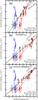 |
Fig. 7 a) Star formation surface density (ΣSFR) as a function of the molecular, atomic, and total hydrogen (H+2H2) gas surface density, as determined by Pineda et al. (2013) in the Galactic plane. b) ΣSFR as function of gas surface density as above, but with the molecular and total hydrogen surface densities calculated by using the 12CO J = 1 → 0 intensity distribution and a constant CO-to-H2 conversion factor of 1.74 × 1020 cm-2 (K km s-1)-1. c) ΣSFR as function of gas surface density as above, but with Σgas derived assuming constant C+ and CO abundances and 12C/13C isotopic ratio. The straight lines are linear fits to the data (with matching color code). We also include the relationships determined for external galaxies by Kennicutt (1998) and Bigiel et al. (2008). All gas surface densities have been corrected to account for the contribution of He. |
In Fig. 7a, we show the relationship between the SFR and the molecular, atomic, and total hydrogen (H+2H2) surface densities as estimated by Pineda et al. (2013). We also include the ΣSFR − Σgas relationship derived for external galaxies by Kennicutt (1998) (for H+2H2) and by Bigiel et al. (2008) (for H2 only). These relationships, and all gas surface densities presented here, have been corrected to account for the contribution of He. Additionally, for comparison, because the extragalactic relationships were derived using different values of XCO, we scaled them so they correspond to those derived using XCO = 1.74 × 1020 cm-2 (K km s-1)-1 (Grenier et al. 2005). The result of the BES fits are listed in Table 2. Using the 12CO, 13CO, and [C ii] to derive the molecular gas surface density results in a relationship with the SFR with a slope ~2 that is steeper than that derived by Bigiel et al. (2008), but one that is consistent with that observed in nearby clouds. Adding the contribution from H to the surface density results in a slope (~3.1) that is steeper than that derived by Kennicutt (1998). As the gas depletion time is defined as  , the steeper slope of the relationship found here implies that the gas is converted into stars at a faster rate in high-Σgas regions. By itself the atomic gas shows no correlation with the SFR. This lack of correlation also holds when we separate the atomic gas in the warm and cold neutral medium components as determined by Pineda et al. (2013).
In Fig. 7b, we show the ΣSFR − Σgas relationship resulting when the molecular gas contribution is estimated by simply multiplying the 12CO emissivity distribution by a constant CO-to-H2 conversion factor, XCO = 1.74 × 1020 cm-2 (K km s-1)-1, a method routinely used in extragalactic studies. We find that the slope of the ΣSFR − Σgas relationship for molecular gas, ~1.0, is in excellent agreement with that derived by Bigiel et al. (2008). Because we use a constant value of XCO, we overestimate the gas surface density as we move inwards in the Galaxy. In the case where the contribution from H i is considered, we find a relationship with a slope ~1.5 that approaches the slope derived by Kennicutt (1998). The differences in the slope resulting from using different approaches to determine the molecular gas surface density suggest that the slopes found in extragalactic studies are strongly influenced by the assumption of a constant XCO factor. External galaxies exhibit a wide range of slopes in the abundance gradients (− 0.1 to −0.9; Moustakas et al. 2010), with the slope we use for the Milky Way (−0.07) being at the lower end of this range. This wide range of slopes can be an important factor contributing to the scatter in the ΣSFR − Σgas relationship observed in large samples of external galaxies, when a constant value of XCO is used. Note that metallicity is often measured in terms of the oxygen abundance, while for the Milky Way we use the slope of the abundance gradient derived by Rolleston et al. (2000) for carbon. The carbon and oxygen abundance gradients might not be necessarily equal considering the different production mechanisms of both elements. However, in the Milky Way, Rolleston et al. (2000) derives an slope for the [O/H] gradient of −0.067 which is similar, within the uncertainties, to that derived for [C/H] (−0.07). Therefore, the results from Rolleston et al. (2000) suggest that the possible difference between [O/H] and [C/H] gradients is not significant. In summary, we suggest that the steeper relationships between ΣSFR and the surface density of molecular gas and total hydrogen (H+2H2) gas found in the Milky Way could also apply to external galaxies.
In Pineda et al. (2013), we showed that XCO varies with Galactocentric distance (see their Fig. 20), and that this variation is mostly produced by the metallicity gradient of the Galaxy, which affects the conversion of the 12CO column density to that of H2. To study the influence of the metallicity gradient, we recalculated the molecular gas surface density assuming constant fractional abundances of [C+]/[H2] = 2.8 × 10⁻⁴ and [CO]/[H2] = 1 × 10⁻⁴ (these values are discussed in Sect. 5.2.2 in Pineda et al. 2013) and a constant 12C/13C isotopic ratio of 65. We compare the SFR and gas surface densities in this case in Fig. 7c. By using a constant abundance, we find relationships with slopes ~1.1 for H2 gas and ~1.6 for H+2H2 gas, which are now consistent with those derived using a constant XCO and therefore with those derived by Bigiel et al. (2008) and Kennicutt (1998). Note that the steeper slope of the ΣSFR − Σgas relationship in Fig. 7a is dominated by the metallicity gradient, with the 12C/13C ratio gradient playing a minor role. The results presented here suggest that metallicity gradients play an important role setting the slope of the relationship between SFR and gas surface densities in galaxies.
The variation of the XCO factor as a function of metallicity in the disk of galaxies has been studied by Sandstrom et al. (2013), see also Magrini et al. (2011), and their results were applied to the ΣSFR − Σgas relationship by Leroy et al. (2013). Sandstrom et al. (2013) find no significant variations in XCO as a function of Galactocentric radius with the exception of the center of galaxies (see also Blanc et al. 2013). Note, however, that the gradient in XCO seen in Pineda et al. (2013) suggest a variation of XCO in the inner Galaxy of about 0.3 dex which is similar to uncertainties in the derivation of XCO in Sandstrom et al. (2013). Thus, if the magnitude of the XCO variations in the inner disk of galaxies are similar to those in the Milky Way, then the gradient would have been obscured by the uncertainties in their derivation of XCO.
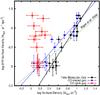 |
Fig. 8 ΣSFR as a function of the CO-dark H2, CO-traced H2, and total molecular gas surface densities, as determined by Pineda et al. (2013). The straight lines are linear fits to the data. We also include the relationship between the SFR and molecular gas surface densities determined for external galaxies by Bigiel et al. (2008). All gas surface densities have been corrected to account for the contribution of He. |
Correlation between the star formation and gas surface densities for different rings in the Galactic plane obtained using BES fits.
In Fig. 8 we show ΣSFR as a function of the CO-dark H2, CO-traced H2 gas, and total molecular gas surface densities, as determined by Pineda et al. (2013). The slope ~2 found for the relationship between star formation and total molecular gas surface density in Fig. 7a is the result of the combination of the contributions from the CO-dark H2 gas and the CO-traced molecular gas. As listed in Table 2, the slope of the relationship involving the CO-traced H2 gas is ~1.3. Although the CO-dark H2 gas is not correlated with the SFR, its contribution makes the slope of the relationship between SFR and total molecular gas steeper, because the CO-dark H2 and CO-traced H2 gas have similar contributions to the total surface density at low values.
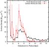 |
Fig. 9 Radial distribution of the azimuthally-averaged surface density of dense molecular gas, derived from C18O observations. We also include the azimuthally-averaged surface density distribution of the total H2 gas derived from 12CO, 13CO, and [C ii] observations which also includes a contribution from diffuse molecular gas. All gas surface densities have been corrected to account for the contribution of He. |
As mentioned above, the relationship between star formation and gas surface density in nearby clouds becomes linear above a certain threshold surface density. Additionally, observations of dense gas tracers (e.g. HCN) also suggest a linear relationship between the dense gas and SFR surface density in local clouds (Wu et al. 2005) and external galaxies (Gao & Solomon 2004). These results indicate that there is a different relationship between star formation and dense molecular gas surface densities compared with that involving the total molecular gas surface density, which also contains diffuse molecular gas. In order to test whether this result also applies to kpc scales in the Galactic plane, we use observations of C18O to derive the radial distribution of the surface density of dense gas as shown in Fig. 9.
Due to its low abundance, large H2 column densities are needed for C18O emission to be detected at the sensitivity of our observations. Molecular clouds are expected to be compact compared with, for example, those of H i gas. Thus, the large H2 column densities required to detect C18O are likely a result of relatively large volume density gas. The C18O observations were taken with the Mopra 20m telescope and are described in Pineda et al. (2013). We first calculated the C18O column density following the procedure described in Pineda et al. (2010, 2013), which first assumes optically thin C18O emission, an excitation temperature derived from 12CO where both this line and C18O are detected, and finally includes an opacity correction. We converted the C18O column density to a 12CO column density using a 12CO/C18O ratio that varies with Galactocentric distance so that it follows the slope derived by Savage et al. (2002) for the 12CO/13CO ratio and corresponds to 12CO/C18O = 557 (Wilson 1999) at Rgal = 8.5 kpc. Similarly, we converted the 12CO column density to that of H2 by applying a [CO]/[H2] gradient with a slope derived by Rolleston et al. (2000) and [CO]/[H2] = 1 × 10⁻⁴ at Rgal = 8.5 kpc. In Fig. 9, we see that the azimuthally-averaged distribution of the dense molecular gas is similar to that of the total molecular gas derived from 12CO, 13CO, and [C ii] (which also includes diffuse molecular gas), but that it extends over a narrower range of Galactocentric radius (4–7 kpc) while showing a pronounced peak at about 4.5 kpc.
In Fig. 10, we show how the surface density of dense H2 gas is related the SFR surface density. We consider rings between 4 and 7 kpc, which correspond to the range where most of the dense H2 gas is detected. The result of the BES fit to the relationship between the dense gas and SFR surface densities is listed in Table 2. Similar to studies of external galaxies and nearby clouds, the dense gas and SFR surface densities are almost linearly correlated in the plane of the Milky Way. We also show in the figure the relationship between star formation and molecular gas (from 12CO and 13CO) to illustrate the difference in the slopes.
The linear correlation between ΣSFR and  can be understood as a consequence of the fact that massive star clusters form nearly exclusively in dense, massive cores. The more dense cores a cloud (or galaxy) has, the more massive stars it will form. The slope of the relationship between ΣSFR and Σgas for the total molecular gas is steeper than that between ΣSFR and because it traces in addition diffuse gas that is not directly associated with star formation but which dominates the gas surface density at low values.
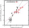 |
Fig. 10 Star formation rate surface density as a function of that of dense molecular gas, as estimated from C18O observations. We also include the ΣSFR − Σgas relationship for the total molecular gas which also accounts for the contribution of diffuse molecular gas. All gas surface densities have been corrected to account for the contribution of He. |
6. Conclusions
In this paper we studied the relationship between the [C ii] emission and SFR in the plane of the Milky Way. We also studied how the SFR surface density is related to that of the different phases of the ISM. We compared these relationships with those observed in external galaxies and local clouds. Our results can be summarized as follows:
-
1.
We find that the[C ii] luminosity and SFR arewell correlated on Galactic scales with a relationship that isconsistent with that found for external galaxies.
-
2.
We find that the [C ii] luminosities arising from the different phases of the ISM are correlated with the SFR, but only the combined emission shows a slope that is consistent with extragalactic observations.
-
3.
We find that the different ISM phases contributing to the total [C ii] luminosity of the Galaxy have roughly comparable contributions: dense PDRs (30%), cold H i (25%), CO-dark H2 (25%), and ionized gas (20%). The contribution from ionized gas to the [C ii] luminosity of the Milky way is larger than that for the emissivity at b = 0° because of the larger scale height of this ISM component relative to the other contributing phases.
-
4.
By combining [C ii] luminosity and SFR data points in the Galactic plane with those observed in external galaxies and nearby star forming regions, we find that a single scaling relationship between the [C ii] luminosity and SFR, log (SFR[M⊙ yr-1]) = (0.89 ± 0.04)log (L[ CII ][erg s-1 ] ) − (36.3 ± 1.5), applies over six orders of magnitude in these quantities.
-
5.
We find that the [C ii] cooling rate for the different contributing ISM components and the SFR are well correlated, as expected for the case of [C ii] cooling balancing the gas heating which is dominated by FUV photons from young stars. The slope in the relationship between cooling rate and SFR is determined by the radial volume density and metallicity gradients.
-
6.
We studied how star formation is related to the gas surface density in the Galactic plane. We find that the SFR and gas surface density relationships show a steeper slope compared to that observed by Kennicutt (1998) and Bigiel et al. (2008), but one that is consistent with that seen in nearby clouds. We find that the different slope is a result of the use of a constant CO-to-H2 conversion factor in the extragalactic studies, which in turn is related to the assumption of constant metallicity in galaxies.
-
7.
We find that the SFR surface density in the Milky way is linearly correlated with that of dense molecular gas, as traced by C18O.
The different scaling relationships between star formation, [C ii] emission, and gas surface density apply over a large range of spatial scales going from those of nearby clouds to those of entire distant galaxies. These multiscale relationships suggest that understanding the process of star formation locally provides insights into the process of star formation in the early universe.
Carbon is ionized by photons with energies ≥11.6 eV and C+ can be excited by collisions with H, H2 and electrons, with critical densities of 3 × 103 cm-3, 6.1 × 103 cm-3 (at Tkin = 100 K), and 44 cm-3 (at Tkin = 8000 K), respectively (see e.g. Goldsmith et al. 2012).
The angular resolution of the Mathewson et al. (1962) and Westerhout (1958) data sets correspond to 40 pc and 50 pc at a distance of 4 kpc from the sun, respectively.
Acknowledgments
This research was conducted at the Jet Propulsion Laboratory, California Institute of Technology under contract with the National Aeronautics and Space Administration. We thank the staffs of the ESA and NASA Herschel Science Centers for their help. We would like to thank Roberto Assef, Moshe Elitzur, Tanio Diaz-Santos, Guillermo Blanc, and Rodrigo Herrera-Camus for enlightening discussions. We also thank an anonymous referee for a number of useful comments.
References
- Akritas, M. G., & Bershady, M. A. 1996, ApJ, 470, 706 [NASA ADS] [CrossRef] [Google Scholar]
- Alves, M. I. R., Davies, R. D., Dickinson, C., et al. 2012, MNRAS, 422, 2429 [NASA ADS] [CrossRef] [Google Scholar]
- Assef, R. J., Kochanek, C. S., Brodwin, M., et al. 2008, ApJ, 676, 286 [NASA ADS] [CrossRef] [Google Scholar]
- Assef, R. J., Kochanek, C. S., Brodwin, M., et al. 2010, ApJ, 713, 970 [NASA ADS] [CrossRef] [Google Scholar]
- Bennett, C. L., Fixsen, D. J., Hinshaw, G., et al. 1994, ApJ, 434, 587 [CrossRef] [Google Scholar]
- Bigiel, F., Leroy, A., Walter, F., et al. 2008, AJ, 136, 2846 [NASA ADS] [CrossRef] [Google Scholar]
- Bigiel, F., Leroy, A. K., Walter, F., et al. 2011, ApJ, 730, L13 [NASA ADS] [CrossRef] [Google Scholar]
- Blanc, G. A., Schruba, A., Evans, II, N. J., et al. 2013, ApJ, 764, 117 [NASA ADS] [CrossRef] [Google Scholar]
- Boselli, A., Gavazzi, G., Lequeux, J., & Pierini, D. 2002, A&A, 385, 454 [NASA ADS] [CrossRef] [EDP Sciences] [Google Scholar]
- Brooks, K. J., Cox, P., Schneider, N., et al. 2003, A&A, 412, 751 [NASA ADS] [CrossRef] [EDP Sciences] [Google Scholar]
- Chomiuk, L., & Povich, M. S. 2011, AJ, 142, 197 [NASA ADS] [CrossRef] [Google Scholar]
- Cordes, J. M., & Lazio, T. J. W. 2002, unpublished [arXiv:astro-ph/0207156] [Google Scholar]
- Cordes, J. M., & Lazio, T. J. W. 2003, unpublished [arXiv:astro-ph/0301598] [Google Scholar]
- Cormier, D., Madden, S. C., Lebouteiller, V., et al. 2014, A&A, 564, A121 [NASA ADS] [CrossRef] [EDP Sciences] [Google Scholar]
- de Graauw, T., Helmich, F. P., Phillips, T. G., et al. 2010, A&A, 518, L6 [NASA ADS] [CrossRef] [EDP Sciences] [Google Scholar]
- de Looze, I., Baes, M., Bendo, G. J., Cortese, L., & Fritz, J. 2011, MNRAS, 416, 2712 [Google Scholar]
- De Looze, I., Cormier, D., Lebouteiller, V., et al. 2014, A&A, 568, A62 [NASA ADS] [CrossRef] [EDP Sciences] [Google Scholar]
- Díaz-Santos, T., Armus, L., Charmandaris, V., et al. 2014, ApJ, 788, L17 [NASA ADS] [CrossRef] [Google Scholar]
- Dickey, J. M., & Lockman, F. J. 1990, ARA&A, 28, 215 [NASA ADS] [CrossRef] [MathSciNet] [Google Scholar]
- Ford, G. P., Gear, W. K., Smith, M. W. L., et al. 2013, ApJ, 769, 55 [NASA ADS] [CrossRef] [Google Scholar]
- Fuchs, B., Jahreiß, H., & Flynn, C. 2009, AJ, 137, 266 [NASA ADS] [CrossRef] [Google Scholar]
- Gao, Y., & Solomon, P. M. 2004, ApJ, 606, 271 [NASA ADS] [CrossRef] [Google Scholar]
- Genzel, R., & Cesarsky, C. J. 2000, ARA&A, 38, 761 [NASA ADS] [CrossRef] [Google Scholar]
- Gold, B., Odegard, N., Weiland, J. L., et al. 2011, ApJS, 192, 15 [Google Scholar]
- Goldsmith, P. F., Langer, W. D., Pineda, J. L., & Velusamy, T. 2012, ApJS, 203, 13 [Google Scholar]
- Grenier, I. A., Casandjian, J.-M., & Terrier, R. 2005, Science, 307, 1292 [NASA ADS] [CrossRef] [PubMed] [Google Scholar]
- Guesten, R., & Mezger, P. G. 1982, Vist. Astron., 26, 159 [Google Scholar]
- Gutermuth, R. A., Pipher, J. L., Megeath, S. T., et al. 2011, ApJ, 739, 84 [NASA ADS] [CrossRef] [Google Scholar]
- Harris, J., & Zaritsky, D. 2009, AJ, 138, 1243 [NASA ADS] [CrossRef] [Google Scholar]
- Heiderman, A., Evans, II, N. J., Allen, L. E., Huard, T., & Heyer, M. 2010, ApJ, 723, 1019 [NASA ADS] [CrossRef] [Google Scholar]
- Heiles, C. 1994, ApJ, 436, 720 [NASA ADS] [CrossRef] [Google Scholar]
- Hill, E. R., Slee, O. B., & Mills, B. Y. 1958, Austr. J. Phys., 11, 530 [Google Scholar]
- Kennicutt, Jr., R. C. 1998, ARA&A, 36, 189 [Google Scholar]
- Kennicutt, R. C., & Evans, N. J. 2012, ARA&A, 50, 531 [NASA ADS] [CrossRef] [Google Scholar]
- Kroupa, P., & Weidner, C. 2003, ApJ, 598, 1076 [NASA ADS] [CrossRef] [Google Scholar]
- Kulkarni, S. R., & Heiles, C. 1987, in Interstellar Processes, eds. D. J. Hollenbach, & H. A. Thronson, Jr., Astrophys. Space Sci. Lib., 134, 87 [Google Scholar]
- Lada, C. J., Lombardi, M., & Alves, J. F. 2010, ApJ, 724, 687 [NASA ADS] [CrossRef] [Google Scholar]
- Langer, W. D., Velusamy, T., Pineda, J. L., et al. 2010, A&A, 521, L17 [Google Scholar]
- Langer, W. D., Pineda, J. L., & Velusamy, T. 2014a, A&A, 564, A101 [NASA ADS] [CrossRef] [EDP Sciences] [Google Scholar]
- Langer, W. D., Velusamy, T., Pineda, J. L., Willacy, K., & Goldsmith, P. F. 2014b, A&A, 561, A122 [NASA ADS] [CrossRef] [EDP Sciences] [Google Scholar]
- Leroy, A. K., Walter, F., Sandstrom, K., et al. 2013, AJ, 146, 19 [NASA ADS] [CrossRef] [Google Scholar]
- Lombardi, M., Bouy, H., Alves, J., & Lada, C. J. 2014, A&A, 566, A45 [NASA ADS] [CrossRef] [EDP Sciences] [Google Scholar]
- Luhman, M. L., Satyapal, S., Fischer, J., et al. 1998, ApJ, 504, L11 [NASA ADS] [CrossRef] [Google Scholar]
- Lyne, A. G., Manchester, R. N., & Taylor, J. H. 1985, MNRAS, 213, 613 [NASA ADS] [CrossRef] [Google Scholar]
- Madden, S. C., Poglitsch, A., Geis, N., Stacey, G. J., & Townes, C. H. 1997, ApJ, 483, 200 [NASA ADS] [CrossRef] [MathSciNet] [Google Scholar]
- Madden, S. C., Rémy-Ruyer, A., Galametz, M., et al. 2013, PASP, 125, 600 [NASA ADS] [CrossRef] [Google Scholar]
- Magrini, L., Bianchi, S., Corbelli, E., et al. 2011, A&A, 535, A13 [NASA ADS] [CrossRef] [EDP Sciences] [Google Scholar]
- Makiuti, S., Shibai, H., Nakagawa, T., et al. 2002, A&A, 382, 600 [NASA ADS] [CrossRef] [EDP Sciences] [Google Scholar]
- Malhotra, S., Helou, G., Stacey, G., et al. 1997, ApJ, 491, L27 [NASA ADS] [CrossRef] [Google Scholar]
- Mathewson, D. S., Healey, J. R., & Rome, J. M. 1962, Austr. J. Phys., 15, 369 [NASA ADS] [CrossRef] [Google Scholar]
- Mezger, P. G., & Smith, L. F. 1976, in Stars and Galaxies from Observational Points of View, ed. E. K. Kharadze, 369 [Google Scholar]
- Mezger, P. O. 1978, A&A, 70, 565 [NASA ADS] [Google Scholar]
- Misiriotis, A., Xilouris, E. M., Papamastorakis, J., Boumis, P., & Goudis, C. D. 2006, A&A, 459, 113 [NASA ADS] [CrossRef] [EDP Sciences] [Google Scholar]
- Moustakas, J., Kennicutt, Jr., R. C., Tremonti, C. A., et al. 2010, ApJS, 190, 233 [NASA ADS] [CrossRef] [Google Scholar]
- Murray, N., & Rahman, M. 2010, ApJ, 709, 424 [NASA ADS] [CrossRef] [Google Scholar]
- Noh, H.-R., & Scalo, J. 1990, ApJ, 352, 605 [NASA ADS] [CrossRef] [Google Scholar]
- Parravano, A., Hollenbach, D. J., & McKee, C. F. 2003, ApJ, 584, 797 [NASA ADS] [CrossRef] [Google Scholar]
- Pilbratt, G. L., Riedinger, J. R., Passvogel, T., et al. 2010, A&A, 518, L1 [CrossRef] [EDP Sciences] [Google Scholar]
- Pineda, J. L., Goldsmith, P. F., Chapman, N., et al. 2010, ApJ, 721, 686 [NASA ADS] [CrossRef] [Google Scholar]
- Pineda, J. L., Langer, W. D., Velusamy, T., & Goldsmith, P. F. 2013, A&A, 554, A103 [NASA ADS] [CrossRef] [EDP Sciences] [Google Scholar]
- Reed, B. C. 2005, AJ, 130, 1652 [NASA ADS] [CrossRef] [Google Scholar]
- Reynolds, R. J. 1989, ApJ, 339, L29 [NASA ADS] [CrossRef] [Google Scholar]
- Rocha-Pinto, H. J., Scalo, J., Maciel, W. J., & Flynn, C. 2000, ApJ, 531, L115 [NASA ADS] [CrossRef] [Google Scholar]
- Rolleston, W. R. J., Smartt, S. J., Dufton, P. L., & Ryans, R. S. I. 2000, A&A, 363, 537 [NASA ADS] [Google Scholar]
- Rubin, D., Hony, S., Madden, S. C., et al. 2009, A&A, 494, 647 [NASA ADS] [CrossRef] [EDP Sciences] [Google Scholar]
- Sandstrom, K. M., Leroy, A. K., Walter, F., et al. 2013, ApJ, 777, 5 [NASA ADS] [CrossRef] [Google Scholar]
- Sargsyan, L., Lebouteiller, V., Weedman, D., et al. 2012, ApJ, 755, 171 [NASA ADS] [CrossRef] [Google Scholar]
- Sargsyan, L., Samsonyan, A., Lebouteiller, V., et al. 2014, ApJ, 790, 15 [NASA ADS] [CrossRef] [Google Scholar]
- Savage, C., Apponi, A. J., Ziurys, L. M., & Wyckoff, S. 2002, ApJ, 578, 211 [NASA ADS] [CrossRef] [Google Scholar]
- Schaerer, D., & Vacca, W. D. 1998, ApJ, 497, 618 [NASA ADS] [CrossRef] [Google Scholar]
- Schmidt, M. 1959, ApJ, 129, 243 [NASA ADS] [CrossRef] [Google Scholar]
- Schneider, N., Stutzki, J., Winnewisser, G., Poglitsch, A., & Madden, S. 1998, A&A, 338, 262 [NASA ADS] [Google Scholar]
- Schruba, A., Leroy, A. K., Walter, F., et al. 2011, AJ, 142, 37 [NASA ADS] [CrossRef] [Google Scholar]
- Smith, L. F., Biermann, P., & Mezger, P. G. 1978, A&A, 66, 65 [NASA ADS] [Google Scholar]
- Smith, L. J., Norris, R. P. F., & Crowther, P. A. 2002, MNRAS, 337, 1309 [NASA ADS] [CrossRef] [Google Scholar]
- Stacey, G. J., Geis, N., Genzel, R., et al. 1991, ApJ, 373, 423 [NASA ADS] [CrossRef] [Google Scholar]
- Stacey, G. J., Jaffe, D. T., Geis, N., et al. 1993, ApJ, 404, 219 [CrossRef] [Google Scholar]
- Stacey, G. J., Hailey-Dunsheath, S., Ferkinhoff, C., et al. 2010, ApJ, 724, 957 [NASA ADS] [CrossRef] [Google Scholar]
- Vutisalchavakul, N., & Evans, II, N. J. 2013, ApJ, 765, 129 [NASA ADS] [CrossRef] [Google Scholar]
- Westerhout, G. 1958, Bull. Astron. Inst. Netherlands, 14, 215 [NASA ADS] [Google Scholar]
- Wiesenfeld, L., & Goldsmith, P. F. 2014, ApJ, 780, 183 [NASA ADS] [CrossRef] [Google Scholar]
- Wilson, T. L. 1999, Rep. Prog. Phys., 62, 143 [Google Scholar]
- Wolfire, M. G., McKee, C. F., Hollenbach, D., & Tielens, A. G. G. M. 2003, ApJ, 587, 278 [NASA ADS] [CrossRef] [Google Scholar]
- Wolfire, M. G., Hollenbach, D., & McKee, C. F. 2010, ApJ, 716, 1191 [NASA ADS] [CrossRef] [Google Scholar]
- Wong, T., & Blitz, L. 2002, ApJ, 569, 157 [NASA ADS] [CrossRef] [Google Scholar]
- Wright, E. L., Mather, J. C., Bennett, C. L., et al. 1991, ApJ, 381, 200 [NASA ADS] [CrossRef] [Google Scholar]
- Wu, J., Evans, II, N. J., Gao, Y., et al. 2005, ApJ, 635, L173 [NASA ADS] [CrossRef] [Google Scholar]
All Tables
Correlation between the [C ii] luminosity of the different contributing ISM components and the SFR for different rings in the Galactic plane obtained using BES fits.
Correlation between the star formation and gas surface densities for different rings in the Galactic plane obtained using BES fits.
All Figures
|
Fig. 1 Upper panel: radial distribution of the free-free emissivity resulting from the average of those from the north and south portions of the Galaxy for Rgal> 2 kpc. Lower panel : radial distribution of the SFR derived following the method described in Sect. 2 for Rgal> 2 kpc. |
| In the text | |
|
Fig. 2 The [C ii] luminosity of the Milky Way as a function of Galactocentric radius. The estimated contributions to the [C ii] luminosity from gas associated with dense PDRs, ionized gas, CNM H i gas, and CO-dark H2 gas are also shown. Typical uncertainties are 5% for the total [C ii] luminosity and the contribution from H i gas, 10% for the contribution from CO-dark H2 gas, and we assume 30% for the contribution from ionized gas. The black dots (and error bars) represent the radial distribution of the SFR derived in Sect. 2. |
| In the text | |
|
Fig. 3 Upper panel: comparison between the SFR and the observed [C ii] luminosity for different rings in the Milky Way. The dashed straight line represents a fit to the data while the solid straight line is the relationship between the SFR and [C ii] luminosity fitted by de Looze et al. (2011) for a set of nearby galaxies. Lower panel: comparison between the SFR surface density and the [C ii] luminosity per unit area. The dashed straight line represents a fit to the data. |
| In the text | |
|
Fig. 4 Star formation rate as a function of [C ii] luminosity for different rings in the Galaxy, the LMC, the galaxies studied by de Looze et al. (2011), and for individual Galactic PDRs. The [C ii] luminosity of the LMC is taken from Rubin et al. (2009) and the SFR from Harris & Zaritsky (2009). The Galactic PDR data points include Orion (L[ CII ] from Stacey et al. 1993, and SFR from Lada et al. 2010), M17 (L[ CII ] from Stacey et al. 1991, and SFR from Lada et al. 2010), Rosette (L[ CII ] from Schneider et al. 1998 and SFR from Chomiuk & Povich 2011), and Carina (L[ CII ] from Brooks et al. 2003 and SFR from Chomiuk & Povich 2011). The [C ii] luminosities and SFRs for this sample are strongly correlated over 6 orders of magnitude. |
| In the text | |
|
Fig. 5 Upper panel: comparison between the SFR and the contribution to the [C ii] luminosity from PDRs and electrons, and bottom panel: from cold H i and CO-dark H2 gas. In both panels the dashed straight lines represent fits to the data and the solid straight line is the relationship between the SFR and [C ii] luminosity fitted by de Looze et al. (2011) in a set of nearby galaxies. Typical uncertainties are 5% for the total [C ii] luminosity and the contribution from H i gas, 10% for the contribution from CO-dark H2 gas, and 30% for the contribution from ionized gas. |
| In the text | |
|
Fig. 6 Upper panel: the [C ii] cooling rate per H atom as a function of the SFR for line-emitting gas associated with dense PDRs, cold H i gas, CO-dark H2 gas, and ionized gas. Lower panel: the [C ii] cooling rate as a function of Galactocentric radius for the different contributing ISM phases discussed in the text. |
| In the text | |
|
Fig. 7 a) Star formation surface density (ΣSFR) as a function of the molecular, atomic, and total hydrogen (H+2H2) gas surface density, as determined by Pineda et al. (2013) in the Galactic plane. b) ΣSFR as function of gas surface density as above, but with the molecular and total hydrogen surface densities calculated by using the 12CO J = 1 → 0 intensity distribution and a constant CO-to-H2 conversion factor of 1.74 × 1020 cm-2 (K km s-1)-1. c) ΣSFR as function of gas surface density as above, but with Σgas derived assuming constant C+ and CO abundances and 12C/13C isotopic ratio. The straight lines are linear fits to the data (with matching color code). We also include the relationships determined for external galaxies by Kennicutt (1998) and Bigiel et al. (2008). All gas surface densities have been corrected to account for the contribution of He. |
| In the text | |
|
Fig. 8 ΣSFR as a function of the CO-dark H2, CO-traced H2, and total molecular gas surface densities, as determined by Pineda et al. (2013). The straight lines are linear fits to the data. We also include the relationship between the SFR and molecular gas surface densities determined for external galaxies by Bigiel et al. (2008). All gas surface densities have been corrected to account for the contribution of He. |
| In the text | |
|
Fig. 9 Radial distribution of the azimuthally-averaged surface density of dense molecular gas, derived from C18O observations. We also include the azimuthally-averaged surface density distribution of the total H2 gas derived from 12CO, 13CO, and [C ii] observations which also includes a contribution from diffuse molecular gas. All gas surface densities have been corrected to account for the contribution of He. |
| In the text | |
|
Fig. 10 Star formation rate surface density as a function of that of dense molecular gas, as estimated from C18O observations. We also include the ΣSFR − Σgas relationship for the total molecular gas which also accounts for the contribution of diffuse molecular gas. All gas surface densities have been corrected to account for the contribution of He. |
| In the text | |
Current usage metrics show cumulative count of Article Views (full-text article views including HTML views, PDF and ePub downloads, according to the available data) and Abstracts Views on Vision4Press platform.
Data correspond to usage on the plateform after 2015. The current usage metrics is available 48-96 hours after online publication and is updated daily on week days.
Initial download of the metrics may take a while.