© ESO, 2014

1. Introduction

One of the well-known properties of rotating stars is their ability to allow matter and angular momentum to be transported across their radiative zone. Indeed, unlike non-rotating stars, a rotating, stably stratified radiative zone cannot be at rest in any (rotating) frame. This property was pointed out long ago by von Zeipel (1924), but refer to Rieutord (2006b) for a recent presentation. The mixing induced by rotation, known as rotational mixing, is usually invoked to explain some features of surface abundances in stars (Li-depletion or nitrogen enrichment for instance). Just as the rotation itself, however, variations of rotation are also known to be an important source of mixing. The spin-down associated with angular momentum loss, itself a consequence of a stellar wind, generates a strong meridional circulation known as Ekman circulation (e.g. Rieutord 1992; Zahn 1992; Rieutord & Zahn 1997).

These features of the dynamics of rotating stars have been included in stellar models using various recipes and assumptions. The main difficulty is that the flows are essentially two-dimensional and therefore can hardly be cast into a one-dimensional model. When this is done, the azimuthal component of the flow field is the only remaining part of the velocity field, which reads v = rΩ(r) sin θe_ϕ. This is the so-called “shellular” differential rotation. The meridional flows cannot be computed as such, since they are intrinsically 2D. Early work (e.g. Pinsonneault 1997) modelled transport as a diffusive process, but Zahn (1992) proposed another approach, now quite popular, which takes the advective process of a meridional circulation into account. Two-dimensional quantities are expanded in spherical harmonics and averaged over isobars. Provided that horizontal diffusion dominates vertical transport, advection of chemical elements by a meridional circulation can be incorporated into a vertical effective diffusion.

The main difficulty with 1D models is that they only apply to slowly rotating stars, since the spherical harmonics series is usually severely truncated (up to ℓ = 2), which produces a poor representation of the Coriolis effect (Rieutord 1987). Actually, the trouble is that we do not know the limiting rotation rate for a reliable use of 1D models making hazardous the use of these models for rapidly rotating stars, or stars that have been rapidly rotating. Thus, even if 1D models have been appropriate guides in the interpretations of abundances observations, a complete understanding of the effects of rotation is still missing.

To go beyond one-dimensional models, we need to study the flows that take place in rotating stars so as to understand their dependence with respect to the main features of stellar conditions (Brunt-Väisälä frequency profiles, turbulence, thermal diffusivity, etc.). This kind of study was initiated by Rieutord (2006a) or Espinosa Lara & Rieutord (2007) with no account of a possible angular momentum loss of the star, however, the spin-down induced by such a process is likely to be a very important part of the dynamics of massive stars (e.g. Lau et al. 2011) or of young stars (Lignières et al. 1996), and therefore deserves a detailed study.

In order to progress in the understanding of the dynamics in these stars, we investigate the effect of the spin-down using a Boussinesq model of a star, thus completing the work of Rieutord (2006a). Although such a model is quite unrealistic as far as direct comparisons to observational data are concerned, it is a useful step to enlight the basic mechanisms operating in a spinning down mass-losing star, and to later deal with more realistic models.

With such a model, we wish to determine the relative influence of baroclinicity and Ekman circulation associated with spin-down on meridional advective transport, and appreciate, when possible, the dynamical consequences of a given mass-loss rate. A review of spin-up/spin-down flows, from the viewpoint of fluid dynamics and including somehow the effect of stratification, may be found in Duck & Foster (2001).

The paper is organized as follows: in the next section, we detail the model that we are using, especially the physics that is included. In the following section, we analyse the spin-down flow when it is either driven by an imposed velocity field at the top of the stellar interior, or when it is driven by stresses imposed by the spinning-down layer where the stellar wind is rooted. The results of the foregoing fluid dynamics section are then discussed in the astrophysical context in term of the wind strength (Sect. 4). We then summarize the hypothesis and results of this work in the last section. The hurried reader solely interested in the astrophysical conclusions may jump directly to this final section.

2. The model

2.1. Description

We consider a self-gravitating, viscous fluid of almost constant density, enclosed in a spherical box of radius R. With this boundary we try to mimic an upper turbulent boundary layer, likely threaded by magnetic fields, which is rotating rigidly or differentially and thickening with time.

The dynamical interaction of a stellar wind with the stellar interior is far from being fully understood. Most studies rely on a global balance of angular momentum (e.g. Zahn 1992; Lau et al. 2011). Following Lignières et al. (2000), we imagine that the friction between the angular momentum losing layer makes it turbulent and that this turbulence entrains lower layers, by the well-known turbulent entrainment process (Turner 1986). The turbulent layer thus slowly deepens while extracting angular momentum from the star’s interior, however, at the same time the star slowly expands as mass is removed, and some outward radial flow also contributes to the spin-down process.

To mimic this complex phenomenon, we assume that the turbulent layer is like a highly viscous fluid that is absorbing some mass flux from the interior. At the interface, the conditions met by the velocity field demands the continuity of both the velocity field and the associated stresses. Since these conditions are quite involved (they need the mean flow field in the turbulent layer), we shall reduce them to two ideal cases: (i) the turbulent layer rotates rigidly and therefore imposes a solid body rotation at the interface, whose angular velocity evolves as , with and ; (ii) the turbulent layer imposes a stress, which brakes the fluid below. In both cases, however, some mass flow crosses the boundary.

Such a modelling is inspired from the work of Friedlander (1976) who considered a similar configuration of a Boussinesq stably stratified fluid inside a sphere, which experiences spin-down by a given surface stress. She discussed this problem using linearized equations thus considering a weak spin-down. One result of this work is that the solutions of this linear problem split into two components: first, a component growing linearly with time and identifiable to a solid body rotation (the actual spinning down rotation) and second, steady, a component made of a meridional circulation that carries the angular momentum, and a differential rotation. As a result, Friedlander (1976) could relate the torque imposed by the surface stress and the angular deceleration of the fluid.

Our rigid condition (i) therefore extends this previous work, but, as we shall see, many features of the solutions are common to the two cases. We sketch out this model in Fig. 1.

2.2. Equations of motion

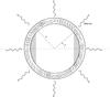Fig. 1 Schematic view of the system: the spinning down turbulent envelope surrounds stably stratified fluid where the spin-down flow develops. The scale-filled outer cylinder of fractional radius s = cosα = 2/$\sqrt{\mathrm{7}}$ is an unstable region that may exist in some cases (see Sect. 3.1.3).

The gravity field inside the fluid is simply g = −g_sr where g_s is the surface gravity and r is the reduced radial coordinate (i.e. r = 0 at the centre and r = 1 at the outer boundary). At equilibrium, the fluid is governed by: 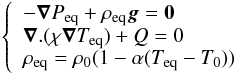$\begin{array}{ccc}\{\begin{array}{c}\\ \\ \\ \end{array}& & \end{array}$(1)where α is the dilation coefficient, χ the thermal conductivity, and Q the heat sinks (inserting heat sinks in the fluid is a trick to impose a stable stratification). Here, P_eq,ρ_eq and T_eq are the equilibrium values of the pressure, density, and temperature respectively. We shall need the Brunt-Väisälä frequency, namely 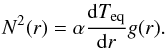$\begin{array}{ccc}{\mathit{N}}^{\mathrm{2}}\mathrm{\left(}\mathit{r}\mathrm{\right)}\mathrm{=}\mathit{\alpha }\frac{\mathrm{d}{\mathit{T}}_{\mathrm{eq}}}{\mathrm{d}\mathit{r}}\mathit{g}\mathrm{\left(}\mathit{r}\mathrm{\right)}\mathit{.}& & \end{array}$(2)As in Rieutord (2006a), we mimic the Brunt-Väisälä frequency profile of stars with the simplified profile shown in Fig. 2.

We now let the system rotate at an angular velocity Ω around the z-axis but, contrary to Rieutord (2006a), we assume that Ω slowly decreases with time, thus 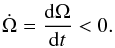$\begin{array}{ccc}\mathrm{\Omega ̇}\mathrm{=}\frac{\mathrm{d\Omega }}{\mathrm{d}\mathit{t}}\mathit{<}\mathrm{0.}& & \end{array}$By slow we mean that , namely that the rotation rates varies very little during a rotation period. In the co-rotating frame, steady flows are the solution to the following equations: 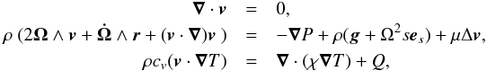$\begin{array}{ccc}{\nabla }\mathrm{·}{v}& \mathrm{=}& \mathrm{0}\mathit{,}\\ \mathit{\rho }\mathrm{(}\mathrm{2}{\Omega }\mathrm{\wedge }{v}\mathrm{+}{\Omega ̇}\mathrm{\wedge }{r}\mathrm{+}\mathrm{(}{v}\mathrm{·}{\nabla }\mathrm{)}{v}\mathrm{)}& \mathrm{=}& \mathrm{-}{\nabla }\mathit{P}\mathrm{+}\mathit{\rho }\mathrm{(}{g}\mathrm{+}{\mathrm{\Omega }}^{\mathrm{2}}\mathit{s}{{e}}_{\mathit{s}}\mathrm{)}\mathrm{+}\mathit{\mu }\mathrm{\Delta }{v}\mathit{,}\\ \mathit{\rho }{\mathit{c}}_{\mathit{v}}\mathrm{(}{v}\mathrm{·}{\nabla }\mathit{T}\mathrm{)}& \mathrm{=}& \end{array}$(3)which express the conservations of mass, momentum, and energy, respectively. There, μ is the dynamical shear viscosity, c_v the specific heat capacity at constant volume, s the radial cylindrical coordinate, and e_s the associated unit vector. These equations differ from those of Rieutord (2006a) by the new term , also called the Euler acceleration. Introducing fluctuations with respect to the equilibrium set-up described by (1) and following Rieutord (2006a) we derive the vorticity equation, which we complete with the equations of energy and mass conservation, namely 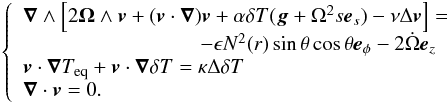$\begin{array}{ccc}\{\begin{array}{c}\\ \\ \\ \\ \end{array}& & \end{array}$(4)Here, κ is the thermal diffusivity, and 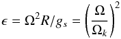$\begin{array}{ccc}\mathit{ϵ}\mathrm{=}{\mathrm{\Omega }}^{\mathrm{2}}\mathit{R}\mathit{/}{\mathit{g}}_{\mathit{s}}\mathrm{=}{\left(\frac{\mathrm{\Omega }}{{\mathrm{\Omega }}_{\mathit{k}}}\right)}^{\mathrm{2}}& & \end{array}$is the ratio of centrifugal acceleration to surface gravity, Ω_k being the associated keplerian angular velocity.

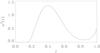Fig. 2 Adopted profile for the Brunt-Väisälä frequency in our calculations. We take the core radius at r = 0.15.

2.3. Scaled equations

Our problem is forced. We need now to scale these equations to get solutions of order unity. Thus, we set 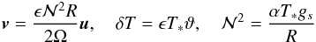$\begin{array}{ccc}{v}\mathrm{=}\frac{\mathit{ϵ}{\mathrm{𝒩}}^{\mathrm{2}}\mathit{R}}{\mathrm{2}\mathrm{\Omega }}{u}\mathit{,} \mathit{\delta T}\mathrm{=}\mathit{ϵ}{\mathit{T}}_{\mathrm{\ast }}\mathit{\vartheta ,} {\mathrm{𝒩}}^{\mathrm{2}}\mathrm{=}\frac{\mathit{\alpha }{\mathit{T}}_{\mathrm{\ast }}{\mathit{g}}_{\mathit{s}}}{\mathit{R}}& & \end{array}$(5)where is the scale of the Brunt-Väisälä frequency. Finally, we obtain the equations for dimensionless dependent variables: 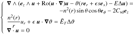$\begin{array}{ccc}\{\begin{array}{c}\\ \\ \\ \\ \end{array}& & \end{array}$(6)where n²(r) is the scaled Brunt-Väisälä frequency, and 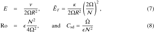$\begin{array}{ccc}\mathit{E}& \mathrm{=}& \frac{\mathit{\nu }}{\mathrm{2}\mathrm{\Omega }{\mathit{R}}^{\mathrm{2}}}\mathit{,} \begin{array}{c}\mathrm{˜}\\ {\mathit{E}}_{\mathit{T}}\end{array}\mathrm{=}\frac{\mathit{\kappa }}{\mathrm{2}\mathrm{\Omega }{\mathit{R}}^{\mathrm{2}}}{\left(\frac{\mathrm{2}\mathrm{\Omega }}{\mathrm{𝒩}}\right)}^{\mathrm{2}}\mathit{,}\\ \mathrm{Ro}& \mathrm{=}& \mathit{ϵ}\frac{{\mathrm{𝒩}}^{\mathrm{2}}}{\mathrm{4}{\mathrm{\Omega }}^{\mathrm{2}}}\mathit{,} \mathrm{and} {\mathit{C}}_{\mathrm{sd}}\mathrm{=}\frac{\mathrm{\Omega ̇}}{\mathit{ϵ}{\mathrm{𝒩}}^{\mathrm{2}}}\end{array}$where E is the Ekman number, which measures the ratio of the viscous force to the Coriolis force, $\begin{array}{c}{\mathrm{˜}}_{}\\ {\mathit{E}}_{\mathit{T}}\end{array}$ measures heat diffusion, Ro is the Rossby number and C_sd is the non-dimensional torque density due to spin-down. For later use we also introduce 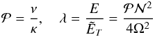$\begin{array}{ccc}\mathrm{𝒫}\mathrm{=}\frac{\mathit{\nu }}{\mathit{\kappa }}\mathit{,} \mathit{\lambda }\mathrm{=}\frac{\mathit{E}}{\begin{array}{c}\mathrm{˜}\\ {\mathit{E}}_{\mathit{T}}\end{array}}\mathrm{=}\frac{\mathrm{𝒫}{\mathrm{𝒩}}^{\mathrm{2}}}{\mathrm{4}{\mathrm{\Omega }}^{\mathrm{2}}}& & \end{array}$(9)namely, the Prandtl number and its product with the scaled Brunt-Väisälä frequency.

2.4. Boundary conditions

System (6) needs to be completed by boundary conditions.

In the first case (i) where the spinning-down layer rotates rigidly and since we are using a frame co-rotating with this layer, the continuity of the velocity field at the interface of the turbulent layer leads to the no-slip conditions¹ on the velocity field. Looking for steady state solutions, we neglect the motion of the interface but include a mass flux at the boundary as in Hypolite & Rieutord (2014). Thus, we impose: $\begin{array}{ccc}{u}\mathrm{=}{\mathit{u}}_{\mathit{e}}{{e}}_{\mathit{r}} \mathrm{at} \mathit{r}\mathrm{=}\mathrm{1.}& & \end{array}$(10)In the second case (ii), we impose the tangential (azimuthal) component of the stress, depending on co-latitude θ, namely $\frac{\mathit{\partial }}{\mathit{\partial r}}\left(\frac{{\mathit{u}}_{\mathit{\varphi }}}{\mathit{r}}\right)\mathrm{=}\mathrm{-}\mathit{\tau }\mathrm{\left(}\mathit{\theta }\mathrm{\right)}\mathit{,} \frac{\mathit{\partial }}{\mathit{\partial r}}\left(\frac{{\mathit{u}}_{\mathit{\theta }}}{\mathit{r}}\right)\mathrm{=}\mathrm{0} \mathrm{at} \mathit{r}\mathrm{=}\mathrm{1}$(11)and ${\mathit{u}}_{\mathit{r}}\mathrm{\left(}\mathrm{1}\mathrm{\right)}\mathrm{=}\mathit{u}e$(12)where we used non-dimensional quantities. The dimensionless stress τ(θ) is related to the dimensional stress τ_∗(θ) by $\mathit{\tau }\mathrm{=}\frac{\mathrm{2}\mathrm{\Omega }{\mathit{\tau }}_{\mathrm{\ast }}}{\mathit{ϵ}{\mathrm{𝒩}}^{\mathrm{2}}\mathit{\mu }}\mathrm{·}$(13)Here, we choose τ ≥ 0 so that condition (11) imposes the braking of the fluid.

As far as the temperature field is concerned, we impose zero temperature fluctuations on this surface, namely $\begin{array}{ccc}\mathit{\vartheta }\mathrm{\left(}\mathrm{1}\mathrm{\right)}\mathrm{=}\mathrm{0.}& & \end{array}$(14)As shown by Friedlander (1976), this condition is of little importance for the flow.

2.5. Relation between spin-down and mass loss

As mentioned above, the expansion of the envelope is also driving a differential rotation and a meridional circulation. To make things tractable, we need to parametrize the mass flux while keeping its association with the direct spin-down drivers (stress or velocity conditions).

To this end, let be the angular momentum loss of the star. This flux is supplied at the base of the turbulent layer (where we set boundary conditions) by a viscous torque and an angular momentum flux associated with the outflowing mass. If we assume that the associated dimensional viscous stress in (11) is τ_∗(θ) = τ_∗ sin θ as suggested by Friedlander (1976), the conservation of angular momentum flux across the layer leads to $\begin{array}{ccc}\mathrm{-}\frac{\mathrm{8}\mathit{\pi }}{\mathrm{3}}{\mathit{R}}^{\mathrm{3}}{\mathit{\tau }}_{\mathrm{\ast }}\mathrm{+}\frac{\mathrm{2}}{\mathrm{3}}\mathit{Ṁ}{\mathit{R}}^{\mathrm{2}}\mathrm{\Omega }\mathrm{=}\mathit{J̇}& & \end{array}$(15)where we assume that the rotation at the boundary is almost uniform. We now parametrize as $\mathit{\beta }\frac{\mathrm{2}}{\mathrm{3}}\mathit{Ṁ}{\mathit{R}}^{\mathrm{2}}\mathrm{\Omega }$. The total angular momentum flux in the layer is therefore split into a fraction β^-1 of simple advection and 1 − β^-1 of viscous stress. We thus write $\begin{array}{ccc}\mathrm{-}\frac{\mathrm{8}\mathit{\pi }}{\mathrm{3}}{\mathit{R}}^{\mathrm{3}}{\mathit{\tau }}_{\mathrm{\ast }}\mathrm{=}\mathrm{(}\mathit{\beta }\mathrm{-}\mathrm{1}\mathrm{)}\frac{\mathrm{2}}{\mathrm{3}}\mathit{Ṁ}{\mathit{R}}^{\mathrm{2}}\mathrm{\Omega }\mathit{.}& & \end{array}$Moving to non-dimensional quantities, the previous equation leads to ${\mathit{u}}_{\mathit{e}}\mathrm{=}\frac{\mathrm{2}\mathit{E\tau }}{\mathit{\beta }\mathrm{-}\mathrm{1}}$(16)which relates the expansion velocity and the stress.

In the case where spin-down is imposed by the velocity field (case (i) of our boundary conditions), things are more involved because we still need the stress to evaluate the angular momentum flux. Since the associated torque is due to the angular deceleration of the turbulent layer, however, dimensional analysis leads to the following equation: $\mathit{k\rho }\mathrm{\Omega ̇}{\mathit{R}}^{\mathrm{5}}\mathrm{+}\frac{\mathrm{2}}{\mathrm{3}}\mathit{Ṁ}{\mathit{R}}^{\mathrm{2}}\mathrm{\Omega }\mathrm{=}\mathit{J̇}\mathit{,}$(17)where k is a non-dimensional constant to be determined from the flow. Introducing parameter β as before, we have $\begin{array}{ccc}\frac{\mathrm{\Omega ̇}}{\mathrm{\Omega }}\mathrm{=}\frac{\mathrm{2}\mathrm{(}\mathit{\beta }\mathrm{-}\mathrm{1}\mathrm{)}}{\mathrm{3}\mathit{k}}\frac{\mathit{Ṁ}}{\mathit{\rho }{\mathit{R}}^{\mathrm{3}}}\mathrm{·}& & \end{array}$Turning to non-dimensional quantities, we find that the expansion velocity is related to the non-dimensional torque density of the spin-down C_sd by ${\mathit{u}}_{\mathit{e}}\mathrm{=}\mathrm{-}\frac{\mathrm{3}\mathit{k}}{\mathrm{4}\mathit{\pi }\mathrm{(}\mathit{\beta }\mathrm{-}\mathrm{1}\mathrm{)}}{\mathit{C}}_{\mathrm{sd}}\mathit{.}$(18)

2.6. Linearization

We shall further simplify the problem by letting and ϵ → 0, but keeping C_sd finite: 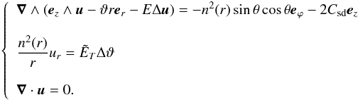$\begin{array}{ccc}\{\begin{array}{c}\\ \\ \\ \\ \\ \end{array}& & \end{array}$(19)These PDE are completed by the following boundary conditions at r = 1: $\begin{array}{ccc}{\mathit{u}}_{\mathit{r}}\mathrm{=}{\mathit{u}}_{\mathit{e}}& & \end{array}$and $\begin{array}{ccc}\frac{\mathit{\partial }}{\mathit{\partial r}}\left(\frac{{\mathit{u}}_{\mathit{\theta }}}{\mathit{r}}\right)\mathrm{=}\mathrm{0} \mathrm{\&} \frac{\mathit{\partial }}{\mathit{\partial r}}\left(\frac{{\mathit{u}}_{\mathit{\varphi }}}{\mathit{r}}\right)\mathrm{=}\mathrm{-}\mathit{\tau }\mathrm{\left(}\mathit{\theta }\mathrm{\right)} \mathrm{or} {\mathit{u}}_{\mathit{\theta }}\mathrm{=}{\mathit{u}}_{\mathit{\varphi }}\mathrm{=}\mathrm{0.}& & \end{array}$We thus get a linear system where the velocity field results from the superposition of three forcings:

• the baroclinic torque −n²(r) sin θ cos θe_ϕ, $\begin{array}{ccc}\mathrm{-}\{\begin{array}{c}\\ \\ \\ \end{array}& & \end{array}$

• the expansion flow.

The effects of the baroclinic torque have been studied in Rieutord (2006a). We thus focus on the spin-down part, which actually contains two drivers: the friction between layers and the expansion flow.

2.7. Typical numbers

Before that and to fix ideas, we computed in Table 1 the main numbers for two ZAMS stars of intermediate masses. These models of solar compositions have been computed with the TGEC code (Toulouse-Geneva Evolution Code, see Hui-Bon-Hoa 2008). From these models, we estimate the typical values of the Brunt-Väisälä frequency squared , the mean Prandtl number , the mean kinematic (radiative) viscosity ⟨ ν ⟩, the typical turbulent values of the kinematic viscosity estimated from Zahn (1992; see below), and the associated Ekman number. We shall also consider two typical rotation periods, namely 0.5 day and 36 days, so as to represent a fast and slow rotation. These figures directly control the λ-parameter, whose two extreme values are given. The rotation period also influences the Ekman number, but in view of the uncertainties on the turbulent transport, we prefer keeping a single value for this parameter. We also give the break-up period below which the star loses mass at its equator (see Rieutord & Espinosa Lara 2013; Espinosa Lara & Rieutord 2013).

3. The spin-down flow

3.1. Driven by velocity boundary conditions

We first concentrate on the case where the outer turbulent layer spins down as a solid body. In a frame co-rotating with this layer, the non-dimensional velocity field u is forced by the torque density −2C_sde_z and meets no-slip boundary conditions with an outflowing mass (10).

3.1.1. Case of a negligible buoyancy

As a first step, we neglect the buoyancy term θ_Tre_r and give below the circumstances in which it is indeed negligible. Thus, we first solve: 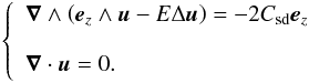$\begin{array}{ccc}\{\begin{array}{c}\\ \\ \\ \end{array}& & \end{array}$(20)System (20) may be solved by a boundary layer analysis in the limit of small Ekman numbers following Rieutord (1987). As in Hypolite & Rieutord (2014), we change the outflow driving of the boundary conditions into a volumic force by setting 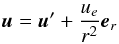$\begin{array}{ccc}{u}\mathrm{=}{{u}}^{\mathrm{\prime }}\mathrm{+}\frac{{\mathit{u}}_{\mathit{e}}}{{\mathit{r}}^{\mathrm{2}}}{{e}}_{\mathit{r}}& & \end{array}$so that (20) now reads 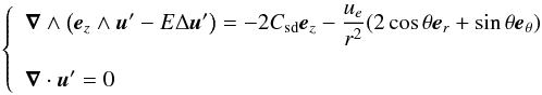$\begin{array}{ccc}\{\begin{array}{c}\\ \\ \\ \end{array}& & \end{array}$(21)and u′ = 0 at r = 1.

When E = 0, these equations are solved by 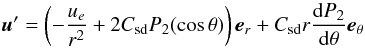${{u}}^{\mathrm{\prime }}\mathrm{=}\left(\mathrm{-}\frac{{\mathit{u}}_{\mathit{e}}}{{\mathit{r}}^{\mathrm{2}}}\mathrm{+}\mathrm{2}{\mathit{C}}_{\mathrm{sd}}{\mathit{P}}_{\mathrm{2}}\mathrm{\left(}\cos \mathit{\theta }\mathrm{\right)}\right){{e}}_{\mathit{r}}\mathrm{+}{\mathit{C}}_{\mathrm{sd}}\mathit{r}\frac{\mathrm{d}{\mathit{P}}_{\mathrm{2}}}{\mathrm{d}\mathit{\theta }}{{e}}_{\mathit{\theta }}$(22)where P₂(cosθ) is the order 2 Legendre polynomial. This flow does not meet the inviscid boundary conditions u′·n = 0 at r = 1, however, it may be viewed as the meridional circulation associated with a differential rotation. In this case we need to evaluate the pumping² of the Ekman layer. In the boundary layer, the flow is ${\mathit{u}}_{\mathrm{0}}\mathrm{+}\begin{array}{c}{}_{\mathrm{˜}}\\ {\mathit{u}}_{\mathrm{0}}\end{array}$, where the boundary layer correction $\begin{array}{c}{\mathrm{˜}}_{}\\ {\mathit{u}}_{\mathrm{0}}\end{array}$ is given by $\begin{array}{ccc}\mathrm{(}{n}\mathrm{\wedge }\begin{array}{c}\mathrm{˜}\\ {\mathit{u}}_{\mathrm{0}}\end{array}\mathrm{+}\mathit{i}\begin{array}{c}\mathrm{˜}\\ {\mathit{u}}_{\mathrm{0}}\end{array}\mathrm{)}\mathrm{=}\mathrm{-}\mathrm{(}{n}\mathrm{\wedge }{\mathit{u}}_{\mathrm{0}}\mathrm{+}\mathit{i}{\mathit{u}}_{\mathrm{0}}{\mathrm{)}}_{\mathit{\alpha }\mathrm{=}\mathrm{0}}\exp \mathrm{(}\mathrm{-}\mathrm{(}\mathrm{1}\mathrm{+}\mathit{i}\mathrm{)}\mathit{\alpha }\mathrm{)}& & \end{array}$(23)where we dropped the primes (in u) and where 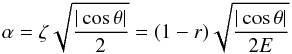$\begin{array}{ccc}\mathit{\alpha }\mathrm{=}\mathit{\zeta }\sqrt{\frac{\mathrm{\left|}\cos \mathit{\theta }\mathrm{\right|}}{\mathrm{2}}}\mathrm{=}\mathrm{(}\mathrm{1}\mathrm{-}\mathit{r}\mathrm{)}\sqrt{\frac{\mathrm{\left|}\cos \mathit{\theta }\mathrm{\right|}}{\mathrm{2}\mathit{E}}}& & \end{array}$(e.g. Greenspan 1969). Identifying the θ and ϕ components of the velocity we get: 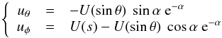$\{\begin{array}{c}\\ {\mathit{u}}_{\mathit{\theta }}& \mathrm{=}& \mathrm{-}\mathit{U}\mathrm{\left(}\sin \mathit{\theta }\mathrm{\right)}\sin \mathit{\alpha }{\mathrm{e}}^{\mathrm{-}\mathit{\alpha }}\\ {\mathit{u}}_{\mathit{\phi }}& \mathrm{=}& \mathit{U}\mathrm{\left(}\mathit{s}\mathrm{\right)}\mathrm{-}\mathit{U}\mathrm{\left(}\sin \mathit{\theta }\mathrm{\right)}\cos \mathit{\alpha }{\mathrm{e}}^{\mathrm{-}\mathit{\alpha }}\end{array}$(24)where the function U(s) is the azimuthal (zero-order) component of the geostrophic flow, which just depends on s, the radial cylindrical coordinate, as imposed by Taylor-Proudman theorem³.

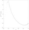Fig. 3 Comparison between the analytical (solid line) and numerical (+) solutions of the equatorial differential rotation of a spin-down flow (E = 10-6 and β = 3). s is the radial coordinate.

The differential equation verified by U(s) is derived from mass conservation in the boundary layer. Indeed, we know that $\mathrm{-}{\mathit{u}}_{\mathit{e}}\mathrm{+}\mathrm{2}{\mathit{C}}_{\mathrm{sd}}{\mathit{P}}_{\mathrm{2}}\mathrm{\left(}\cos \mathit{\theta }\mathrm{\right)}\mathrm{+}\begin{array}{c}\mathrm{˜}\\ {\mathit{u}}_{\mathit{r}}\end{array}\mathrm{=}\mathrm{0} \mathrm{at} \mathit{r}\mathrm{=}\mathrm{1}$(25)A ζ-integration of the continuity equation leads to 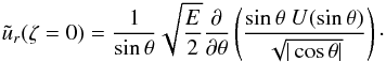$\begin{array}{ccc}\begin{array}{c}\mathrm{˜}\\ {\mathit{u}}_{\mathit{r}}\end{array}\mathrm{(}\mathit{\zeta }\mathrm{=}\mathrm{0}\mathrm{)}\mathrm{=}\frac{\mathrm{1}}{\sin \mathit{\theta }}\sqrt{\frac{\mathit{E}}{\mathrm{2}}}\frac{\mathit{\partial }}{\mathit{\partial \theta }}\left(\frac{\sin \mathit{\theta }\mathit{U}\mathrm{\left(}\sin \mathit{\theta }\mathrm{\right)}}{\sqrt{\mathrm{\left|}\cos \mathit{\theta }\mathrm{\right|}}}\right)\mathrm{·}& & \end{array}$Using (25), we finally get

$\mathit{U}\mathrm{\left(}\mathit{s}\mathrm{\right)}\mathrm{=}\mathrm{-}{\mathit{C}}_{\mathrm{sd}}\sqrt{\frac{\mathrm{2}}{\mathit{E}}}\frac{\mathrm{(}\mathrm{1}\mathrm{-}{\mathit{s}}^{\mathrm{2}}{\mathrm{)}}^{\mathrm{3}\mathit{/}\mathrm{4}}}{\mathit{s}}\left(\frac{{\mathit{u}}_{\mathit{e}}}{{\mathit{C}}_{\mathrm{sd}}}\mathrm{+}{\mathit{s}}^{\mathrm{2}}\right)\mathrm{·}$(26)From solution (26) and expressions (24), the viscous torque applied to the outer turbulent layer can be evaluated. It gives the nondimensional constant k of (17). It turns out that $\begin{array}{ccc}\mathit{k}\mathrm{=}\frac{\mathrm{8}\mathit{\pi }}{\mathrm{15}}\left(\mathrm{1}\mathrm{-}\frac{\mathrm{1}}{\mathit{\beta }}\right)& & \end{array}$and ${\mathit{u}}_{\mathit{e}}\mathrm{=}\mathrm{-}\frac{\mathrm{2}{\mathit{C}}_{\mathrm{sd}}}{\mathrm{5}\mathit{\beta }}$(27)therefore $\mathit{U}\mathrm{\left(}\mathit{s}\mathrm{\right)}\mathrm{=}\mathrm{-}{\mathit{C}}_{\mathrm{sd}}\sqrt{\frac{\mathrm{2}}{\mathit{E}}}\frac{\mathrm{(}\mathrm{1}\mathrm{-}{\mathit{s}}^{\mathrm{2}}{\mathrm{)}}^{\mathrm{3}\mathit{/}\mathrm{4}}}{\mathit{s}}\left(\mathrm{-}\frac{\mathrm{2}}{\mathrm{5}\mathit{\beta }}\mathrm{+}{\mathit{s}}^{\mathrm{2}}\right)\mathrm{·}$(28)We note that this solution is singular on the rotation axis because of the singular nature of the outflow at r = 0. In the numerics, we remove this singularity by assuming that the outflow starts at some finite radius (a core-envelope boundary here at r = 0.15). Figure 3 shows a comparison between the analytic and numerical solutions. At E = 10^-6, the difference in the envelope is hardly perceptible. Figure 4 illustrates the associated meridional circulation.

Fig. 4 Meridional circulation associated with a spin-down flow in the case of Fig. 3. The dotted isocontours show a clockwise circulation, while the solid lines are for anti-clockwise circulation. Numerical resolution used Nr = 150 Chebyshev polynomials radially and spherical harmonics up to order L = 160.

The foregoing analytical solution does not take the effects of buoyancy into account. However, these effects can be neglected in some range of parameters. Let us first observe that the meridional circulation induced by the spin-down should be associated with a temperature fluctuation that verifies $\begin{array}{ccc}{\mathit{\theta }}_{\mathit{T}}\mathrm{~}\frac{{\mathit{C}}_{\mathrm{sd}}}{\begin{array}{c}\mathrm{˜}\\ {\mathit{E}}_{\mathit{T}}\end{array}}\mathrm{=}{\mathit{C}}_{\mathrm{sd}}\mathit{\lambda }\mathit{/}\mathit{E}& & \end{array}$as given by the energy equation in (19). Since the Coriolis term is , the buoyancy can be neglected in the momentum equation if θ_T ≪ C_sdE^{− 1/2} or when $\mathit{\lambda }\mathrm{\ll }\sqrt{\mathit{E}}\mathit{.}$(29)This constraint is obviously not met in radiative region of the 3 M_⊙ star, but can be met in massive stars rotating near breakup as shown by the 7 M_⊙ model numbers.

We now further explore the properties of solution (28) in order to have a reference for numerical solutions. It will also turn out that some properties carry on in the domain of full coupling when $\mathit{\lambda }\gtrsim \sqrt{\mathit{E}}$.

3.1.2. Baroclinicity versus spin-down

The foregoing results allow us to determine the range of parameters where either baroclinicity or spin-down dominate the driving of the flows.

With the scaling leading to (19), the differential rotation arising from baroclinicity is of order unity (see Rieutord 2006a). Thus, from (28), we see that the differential rotation driven by the spin-down dominates if $\frac{{\mathit{C}}_{\mathrm{sd}}}{\sqrt{\mathit{E}}}\mathrm{\gg }\mathrm{1.}$(30)Joining this condition with (29), we find that the influence of a stable stratification on the differential rotation triggered by a spin-down is negligible when ${\mathit{C}}_{\mathrm{sd}}\mathrm{\gg }\sqrt{\mathit{E}}\mathrm{\gg }\mathit{\lambda }\mathit{.}$(31)Besides, the meridional circulation associated with the spin-down flow is as given by (22). It overwhelms the baroclinic circulation, which is , if ${\mathit{C}}_{\mathrm{sd}}\mathrm{\gg }\mathit{E}$(32)Since E ≪ 1, when (30) is met, (32) is also met. In this case, the flow is completely dominated by the spin-down flow. For a weaker spin-down, such that $\mathit{E}\mathrm{\ll }{\mathit{C}}_{\mathrm{sd}}\mathrm{\ll }\sqrt{\mathit{E}}$(33)the meridional circulation is triggered by the spin-down, while the differential rotation is essentially coming from the baroclinic torque. This result shows that the meridional circulation driven by baroclinicity is actually extremely weak because Ekman numbers are usually less than 10^-8.

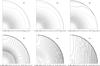Fig. 5 Differential rotation of a stably stratified rotating fluid in a sphere when the spin-down forcing Csd is strengthened. From left to right and top to bottom Csd = 0, − 10-6, − 10-5, − 10-4, − 10-3, − 10-2. Ekman and Prandtl numbers are E = 10-7, Pr = 10-4. All calculations have assumed β ≫ 1. Solid lines are for positive values, dotted for negative values. Numerical resolution used Nr = 200 Chebyshev polynomials radially and spherical harmonics up to order L = 250.

Fig. 6 Meridional circulation in a stably stratified rotating fluid in a sphere when the spin-down forcing Csd is increased (Csd = 0,10-6,10-5from left to right). Streamlines of the meridional circulations are shown in the same way as in Fig. 4. As in Fig. 5, E = 10-7, Pr = 10-4, and β ≫ 1. Numerical resolution is the same as in Fig. 5.

The foregoing inequalities show that three regimes may be distinguished: a strong wind regime occurs when (30) is verified, namely when the spin-down flows dominate both the circulations and the differential rotation, a moderate wind regime described by (33), when meridional circulation is that imposed by the spin-down and the differential rotation is controlled by baroclinicity, and finally a weak or null-wind regime when baroclinic flows are only slightly perturbed by the spin-down.

In Figs. 5 and 6, we illustrate this case where $\mathit{\lambda }\mathrm{\ll }\sqrt{\mathit{E}}$ so that the buoyancy is negligible and the analytic solution applies. We choose λ = 10^-4 and E = 10^-7 for various values of C_sd. The figures clearly illustrate the transitions that are expected from analytics, namely that, as the spin-down forcing increases, the meridional circulation first transits to the spin-down meridional circulation around C_sd = 10^-6, while the differential rotation reaches the asymptotic state enforced by spin-down when ${\mathit{C}}_{\mathrm{sd}}\gtrsim \sqrt{\mathit{E}}$.

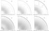Fig. 7 Differential rotation when the spin-down forcing Csd is strengthened while the buoyancy is influential. From left to right and top to bottom Csd = 0, − 10-6, − 10-5, − 10-4, − 10-3, − 10-2 We use E = 10-7, Pr = 3 × 10-2, $\mathit{\lambda }\mathrm{\simeq }\mathrm{3}\mathrm{\times }{\mathrm{10}}^{-2}\mathrm{=}\mathrm{100}\sqrt{\mathit{E}}$ and β ≫ 1. Top row: the flow is dominated by the baroclinic forcing. Bottom row: the flow is dominated by the spin-down forcing. Numerical resolution is the same as in Fig. 5.

3.1.3. Centrifugal instability

With the analytic expression of the azimuthal velocity (28) we can determine the conditions of the appearance of the centrifugal instability. Indeed, when the specific angular momentum of the fluid decreases with the distance to the axis, axisymmetric disturbances can grow. Noting that the specific angular momentum ℓ reads $\begin{array}{ccc}\mathit{\ell }\mathrm{=}{\mathit{s}}^{\mathrm{2}}\mathrm{+}\mathit{sU}\mathrm{\left(}\mathit{s}\mathrm{\right)}\mathit{,}& & \end{array}$the condition dℓ/ds ≤ 0 leads to $\mathrm{(}\mathrm{1}\mathrm{-}{\mathit{s}}^{\mathrm{2}}{\mathrm{)}}^{\mathrm{1}\mathit{/}\mathrm{4}}\mathrm{\le }\mathrm{|}{\mathit{C}}_{\mathrm{sd}}\mathrm{|}\sqrt{\frac{\mathrm{2}}{\mathit{E}}}\left(\frac{\mathrm{7}}{\mathrm{4}}{\mathit{s}}^{\mathrm{2}}\mathrm{-}\mathrm{1}\mathrm{+}\frac{\mathrm{3}}{\mathrm{10}\mathit{\beta }}\right)\mathit{,}$(34)which determines the region where the centrifugal instability develops.

If $\mathrm{\left|}{\mathit{C}}_{\mathrm{sd}}\mathrm{\right|}\mathrm{\ll }\sqrt{\mathit{E}}$, namely in the moderate wind condition, (34) only applies to a very small fraction of the volume. Indeed, the centrifugal instability develops when $\begin{array}{ccc}\mathit{s}\mathrm{\ge }\mathrm{1}\mathrm{-}\mathrm{𝒪}\mathrm{(}{\mathit{C}}_{\mathrm{sd}}^{\mathrm{4}}\mathit{/}{\mathit{E}}^{\mathrm{2}}\mathrm{)}\mathit{.}& & \end{array}$If we observe that this condition applies outside the Ekman layer, we need demanding ${\mathit{C}}_{\mathrm{sd}}^{\mathrm{4}}\mathit{/}{\mathit{E}}^{\mathrm{2}}\mathit{>}{\mathit{E}}^{\mathrm{1}\mathit{/}\mathrm{2}}$ or that $\begin{array}{ccc}{\mathit{E}}^{\mathrm{5}\mathit{/}\mathrm{8}}\mathit{<}{\mathit{C}}_{\mathrm{sd}}\mathit{<}{\mathit{E}}^{\mathrm{1}\mathit{/}\mathrm{2}}\mathit{,}& & \end{array}$which quite restricts the range of acceptable C_sd-values. Hence, in the moderate wind regime, the influence of the centrifugal instability is likely marginal.

On the other hand, in the strong wind regime, we only demand that the rhs of (34) be positive so that all the volume beyond $\begin{array}{ccc}{\mathit{s}}_{\mathit{m}}\mathrm{=}\frac{\mathrm{2}}{\sqrt{\mathrm{7}}}\left(\mathrm{1}\mathrm{-}\frac{\mathrm{3}}{\mathrm{20}\mathit{\beta }}\right)& & \end{array}$can develop the centrifugal instability. This region of the star is sketched out in Fig. 1 for infinite β. We thus expect that equatorial regions are more mixed than the polar regions.

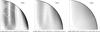Fig. 8 Change in the meridional circulation when the spin-down forcing is increased. We represent the streamlines of the meridional circulation for Csd = 0,10-6,10-5from left to right. As in Fig. 7E = 10-7, Pr = 3 × 10-2 and β ≫ 1. Solid line show counter-clockwise circulation. Numerical resolution is the same as in Fig. 5.

3.1.4. The influence of buoyancy

The foregoing derivation neglected the coupling of the spin-down flow with the temperature field, which occurs through buoyancy. As already noticed, this is not possible in the radiative region of stars when $\mathit{\lambda }\mathrm{\gg }\sqrt{\mathit{E}}$.

To investigate the fully coupled case, we resort to numerical solutions of the complete system (19). The numerical method is the same as in Rieutord (2006a) and will not be repeated here. It is based on a spectral method that uses spherical harmonics to represent the angular variations of the solutions and Chebyshev polynomials for the radial dependence.

In Fig. 7, as in Fig. 5, we investigate the transition from a pure baroclinic flow to a spin-down dominated flow. Obviously, the flow also makes this transition for values ${\mathit{C}}_{\mathrm{sd}}\mathrm{~}\sqrt{\mathit{E}}$ but reaches a new state close to a shellular rotation, especially in the central region.

The meridian streamlines, depicted in Fig. 8, show a transition to the spin-down dominated state at a lower value of C_sd, as in the uncoupled case.

The foregoing shellular rotation can be understood from (19), if we neglect the viscosity. The vorticity equation now reads: $\begin{array}{ccc}\frac{\mathit{\partial }{u}}{\mathit{\partial z}}\mathrm{=}\mathrm{(}{\mathit{\partial }}_{\mathit{\theta }}\mathit{\vartheta }\mathrm{+}{\mathit{n}}^{\mathrm{2}}\mathrm{(}\mathit{r}\mathrm{\left)}\sin \mathit{\theta }\cos \mathit{\theta }\mathrm{\right)}{{e}}_{\mathit{\varphi }}\mathrm{+}\mathrm{2}{\mathit{C}}_{\mathrm{sd}}{{e}}_{\mathit{z}}\mathit{.}& & \end{array}$Considering that the meridional circulation (22) compensates the spin-down torque 2C_sde_z, we note that the radial component reads u_r = C_sdr(3cos²θ − 1) = 2rC_sdP₂(cosθ). We easily see that the temperature perturbation associated with this circulation reads: $\begin{array}{ccc}\mathit{\vartheta }\mathrm{=}\frac{{\mathit{C}}_{\mathrm{sd}}}{\begin{array}{c}\mathrm{˜}\\ {\mathit{E}}_{\mathit{T}}\end{array}}{\mathit{\vartheta }}_{\mathrm{2}}\mathrm{\left(}\mathit{r}\mathrm{\right)}{\mathit{P}}_{\mathrm{2}}\mathrm{\left(}\cos \mathit{\theta }\mathrm{\right)}& & \end{array}$where ϑ₂(r) is a function determined by the Brunt-Väisälä frequency profile n²(r). When the amplitude of the temperature perturbation ${\mathit{C}}_{\mathrm{sd}}\mathit{/}\begin{array}{c}{}_{\mathrm{˜}}\\ {\mathit{E}}_{\mathit{T}}\end{array}$ is larger than unity, the baroclinic torque generated by the spin-down flow overwhelms the baroclinic torque resulting from the centrifugal force, −n²(r) sin θ cos θe_ϕ. This leads to an azimuthal velocity that may be written $\begin{array}{ccc}{\mathit{u}}_{\mathit{\varphi }}\mathrm{=}\frac{{\mathit{C}}_{\mathrm{sd}}}{\begin{array}{c}\mathrm{˜}\\ {\mathit{E}}_{\mathit{T}}\end{array}}\mathrm{\Omega }\mathrm{\left(}\mathit{r}\mathrm{\right)}\sin \mathit{\theta }\mathrm{+}\mathit{U}\mathrm{\left(}\mathit{s}\mathrm{\right)}& & \end{array}$where U(s) is the geostrophic flow that makes the boundary conditions verified and Ω(r) is determined by ϑ₂(r). If U is small enough, we see that a shellular differential rotation naturally emerges. This seems to be the case for the values chosen in Fig. 7.

If u_ϕ is $\mathrm{𝒪}\mathrm{(}{\mathit{C}}_{\mathrm{sd}}\mathit{/}\begin{array}{c}{\mathrm{˜}}_{}\\ {\mathit{E}}_{\mathit{T}}\end{array}\mathrm{)}$, internal balance of viscous force and Coriolis force gives a radial flow that is $\mathrm{𝒪}\mathrm{(}\mathit{E}{\mathit{C}}_{\mathrm{sd}}\mathit{/}\begin{array}{c}{\mathrm{˜}}_{}\\ {\mathit{E}}_{\mathit{T}}\end{array}\mathrm{)}$ or . On the other hand, Ekman pumping generates a $\mathrm{𝒪}\mathrm{(}\sqrt{\mathit{E}}{\mathit{C}}_{\mathrm{sd}}\mathit{/}\begin{array}{c}{\mathrm{˜}}_{}\\ {\mathit{E}}_{\mathit{T}}\end{array}\mathrm{)}$ or $\mathrm{𝒪}\mathrm{(}\mathit{\lambda }{\mathit{C}}_{\mathrm{sd}}\mathit{/}\sqrt{\mathit{E}}\mathrm{)}$ circulation. Numerical solutions show that the baroclinic circulation still disappears when C_sd>E, indicating that Ekman pumping is weak (it can be zero if the latitudinal flow varies appropriately) and therefore that condition (32), determining the domination of the spin-down driven circulation, likely extends for all λ less than unity.

3.2. Stress-driven spin-down

The case of a stress-driven spin-down has been fully analysed by Friedlander (1976), focusing on the slowing down rotation of the radiative zone of the Sun. We shall not repeat this complex analysis, but focus directly on our original question as to which condition characterizes the dominance of spin-down circulation compared to the baroclinic circulation.

For this, we reconsider the boundary layer analysis of Rieutord (2006a) in Sect. 3.2. The stress-free boundary conditions are now modified into $\frac{\mathit{\partial }}{\mathit{\partial r}}\left(\frac{{\mathit{u}}_{\mathit{\theta }}\mathrm{+}\mathit{i}{\mathit{u}}_{\mathit{\varphi }}}{\mathit{r}}\right)\mathrm{=}\mathrm{-}\mathit{i\tau }\mathrm{\left(}\mathit{\theta }\mathrm{\right)}$(35)where τ is the non-dimensional surface stress. The general expression of the flow in the Ekman layer is $\begin{array}{ccc}{\mathit{u}}_{\mathit{\theta }}\mathrm{+}\mathit{i}{\mathit{u}}_{\mathit{\varphi }}\mathrm{=}\mathit{C}\exp \left(\mathrm{-}\mathit{\zeta }\sqrt{\mathit{i}\mathrm{\left|}\cos \mathit{\theta }\mathrm{\right|}}\right)\mathrm{+}\mathit{i}{\mathit{u}}_{\mathit{\varphi }}^{\mathrm{0}}& & \end{array}$where ${\mathit{u}}_{\mathit{\varphi }}^{\mathrm{0}}$ is the interior inviscid solution that reads 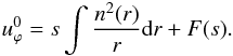$\begin{array}{ccc}{\mathit{u}}_{\mathit{\varphi }}^{\mathrm{0}}\mathrm{=}\mathit{s}\mathrm{\int }\frac{{\mathit{n}}^{\mathrm{2}}\mathrm{\left(}\mathit{r}\mathrm{\right)}}{\mathit{r}}\mathrm{d}\mathit{r}\mathrm{+}\mathit{F}\mathrm{\left(}\mathit{s}\mathrm{\right)}\mathit{.}& & \end{array}$The constant C is such that condition (35) is met. This leads to $\begin{array}{ccc}\mathit{C}\mathrm{\equiv }\mathit{C}\mathrm{\left(}\mathit{\theta }\mathrm{\right)}\mathrm{=}\mathrm{(}\mathrm{1}\mathrm{+}\mathit{i}\mathrm{)}\sqrt{\frac{\mathit{E}}{\mathrm{2}}}\mathrm{\Gamma }\mathrm{\left(}\mathit{\theta }\mathrm{\right)}& & \end{array}$with $\begin{array}{ccc}\mathrm{\Gamma }\mathrm{\left(}\mathit{\theta }\mathrm{\right)}\mathrm{=}\frac{\mathit{F}\mathrm{\left(}\sin \mathit{\theta }\mathrm{\right)}\mathrm{-}\sin \mathit{\theta }{\mathit{F}}^{\mathrm{\prime }}\mathrm{\left(}\sin \mathit{\theta }\mathrm{\right)}\mathrm{-}{\mathit{n}}^{\mathrm{2}}\mathrm{\left(}\mathrm{1}\mathrm{\right)}\sin \mathit{\theta }\mathrm{-}\mathit{\tau }\mathrm{\left(}\mathit{\theta }\mathrm{\right)}}{\sqrt{\mathrm{\left|}\cos \mathit{\theta }\mathrm{\right|}}}& & \end{array}$(36)where the prime indicates a derivative.

From this latter expression, it is clear that the stress driving will overtake the baroclinic driving when $\begin{array}{ccc}\mathit{\tau }\mathrm{\gg }{\mathit{n}}^{\mathrm{2}}\mathrm{\left(}\mathrm{1}\mathrm{\right)}\mathrm{~}\mathrm{1.}& & \end{array}$Indeed, the scaling has been chosen such that n²(r) is . We further note that when this inequality is met, both the circulation and the differential rotation overtake their baroclinic equivalent. This is because both flows meet boundary conditions on the stress.

As shown by Friedlander (1976), the radial driving of the circulation by the pumping of the boundary layer is similar as in the velocity driven case if τ(θ) = τ_e sin θ. In this case, one finds $\begin{array}{ccc}\begin{array}{c}\mathrm{˜}\\ {\mathit{u}}_{\mathit{r}}\end{array}\mathrm{=}\mathrm{-}\mathit{E}{\mathit{\tau }}_{\mathit{e}}{\mathit{P}}_{\mathrm{2}}\mathrm{\left(}\cos \mathit{\theta }\mathrm{\right)}& & \end{array}$similar to expression (25) when β ≫ 1.

4. Discussion

We now replace the foregoing results in the astrophysical context.

4.1. Stress-driven spin-down

4.1.1. A transition mass-loss rate

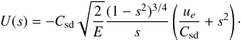
We may estimate the stress imposed by the turbulent layer if we follow the result of Lignières et al. (2000) that the angular velocity profile is such that the specific angular momentum in the layer remains constant. In such a case, ${\mathrm{\Omega }}_{\mathit{l}}\mathrm{\left(}\mathit{s}\mathrm{\right)}\mathrm{\propto }{\mathit{s}}^{-2}\mathit{,}$(37)and the azimuthal stress is $\begin{array}{ccc}{\mathit{\tau }}_{\mathrm{\ast }}\mathrm{=}{\mathit{\mu }}_{\mathit{t}}\mathit{s}\frac{\mathit{\partial }}{\mathit{\partial s}}\frac{{\mathit{v}}_{\mathit{\varphi }}}{\mathit{s}}\mathrm{=}\mathrm{-}\mathrm{2}{\mathit{\mu }}_{\mathit{t}}{\mathrm{\Omega }}_{\mathit{l}}\mathrm{\left(}\mathit{s}\mathrm{\right)}& & \end{array}$so that at the interface $\begin{array}{ccc}{\mathit{\tau }}_{\mathrm{\ast }}\mathrm{=}\mathrm{-}\mathrm{2}\mathrm{\Omega }{\mathit{\mu }}_{\mathit{t}}& & \end{array}$where Ω is the angular velocity of the fluid at the interface and μ_t is the turbulent viscosity.

If we further assume that the turbulent layer propagates in a stably stratified envelope without removing the stable stratification⁴, we can use the turbulent viscosity of Zahn’s model (Zahn 1992), namely $\begin{array}{ccc}{\mathit{\mu }}_{\mathit{t}}\mathrm{=}\mathit{\rho }\frac{\mathrm{Ri}\mathrm{c}\mathit{\kappa }}{\mathrm{3}}{\left(\frac{\mathit{s}}{\mathrm{𝒩}}\frac{\mathrm{d\Omega }}{\mathrm{d}\mathit{s}}\right)}^{\mathrm{2}}& & \end{array}$where Ri_c is the critical Richardson number. Assuming that the angular velocity profile verifies (37) and that Ri_c ~ 1/4, we get ${\mathit{\mu }}_{\mathit{t}}\mathrm{~}\frac{\mathit{\rho \kappa }}{\mathrm{12}}{\left(\frac{\mathrm{2}\mathrm{\Omega }}{\mathrm{𝒩}}\right)}^{\mathrm{2}}\mathrm{·}$(38)Note that the place where the boundary conditions are taken is arbitrary within the turbulent layer. The stress at the interface is ${\mathit{\tau }}_{\mathrm{\ast }}\mathrm{~}\mathrm{-}\frac{\mathit{\rho \kappa }\mathrm{\Omega }}{\mathrm{6}}{\left(\frac{\mathrm{2}\mathrm{\Omega }}{\mathrm{𝒩}}\right)}^{\mathrm{2}}\mathrm{·}$(39)We note that the Ekman number associated with this turbulent viscosity is ${\mathit{E}}_{\mathit{t}}\mathrm{=}\frac{{\mathit{\nu }}_{\mathit{t}}}{\mathrm{2}\mathrm{\Omega }{\mathit{R}}^{\mathrm{2}}}\mathrm{~}\frac{\mathit{\kappa }}{\mathrm{24}\mathrm{\Omega }{\mathit{R}}^{\mathrm{2}}}{\left(\frac{\mathrm{2}\mathrm{\Omega }}{\mathrm{𝒩}}\right)}^{\mathrm{2}}\mathrm{=}\begin{array}{c}\mathrm{˜}\\ {\mathit{E}}_{\mathit{T}}\end{array}\mathit{/}\mathrm{12}$(40)thus $\begin{array}{ccc}\mathit{\lambda }\mathrm{~}\mathrm{1}\mathit{/}\mathrm{12}& & \end{array}$when turbulence is fully developed. In passing, we note that the ratio between viscosity and turbulent viscosity is $\frac{\mathit{\mu }}{{\mathit{\mu }}_{\mathit{t}}}\mathrm{~}\mathrm{12}\mathit{\lambda }\mathit{.}$(41)Turbulence only increases momentum transport in fast rotating stars where 12λ< 1 (typically rotation periods less than 30 days).

Expression (39) shows that the stress imposed by the turbulence is determined by the local physical conditions of the interface.

We now reconsider the balance of angular momentum (15) together with (39). From the definition of β, we get the expression $\mathit{\beta }\mathrm{=}\mathrm{1}\mathrm{+}\frac{\mathrm{\left|}\mathit{Ṁ}\mathit{t}\mathrm{\right|}}{\mathrm{\left|}\mathit{Ṁ}\mathrm{\right|}}$(42)where we introduced the “transition” mass-loss rate $\mathit{Ṁ}\mathit{t}\mathrm{=}\frac{\mathrm{2}\mathit{\pi }}{\mathrm{3}}\mathit{\rho \kappa R}{\left(\frac{\mathrm{2}\mathrm{\Omega }}{\mathrm{𝒩}}\right)}^{\mathrm{2}}\mathrm{·}$(43)This expression shows that a characteristic mass flux exists that determines whether transport of angular momentum is dominated by advection or turbulent viscous diffusion. This is a consequence of the assumptions (37) together with the turbulence model. They make the turbulent angular momentum flux due to diffusion depending only on local conditions. Hence, the adjustment to the actual angular momentum loss rate is made by advection. Our restriction β ≫ 1 therefore selects mass losses smaller than | Ṁ_t |. The range | Ṁ | > | Ṁ_t | therefore naturally delineates a strong wind regime.

In Table 2, we have computed the transition mass-loss rate for our two stellar models. Quite remarkably, we find that the values are insensitive to the depth of the layer. This is because ρκ (the product of density and thermal diffusivity) is almost constant in the upper half (in radius) of the star (see Fig. 9). We find ρκ ~ 10⁸ cgs for the 3 M_⊙ star and ρκ ~ 10⁹ cgs for the 7 M_⊙ star.

The values of Table 2 show that for fast rotating stars rather strong winds are necessary to make advection dominating.

4.1.2. Baroclinic and spin-down flows

We now assume that the bulk of the star is decelerated by the turbulent stress of the upper layers, namely by ${\mathit{\tau }}_{\mathrm{\ast }}\mathrm{~}\mathrm{2}{\mathit{\mu }}_{\mathit{t}}\mathrm{\Omega }\mathit{.}$(44)The condition by which the spin-down flow supersedes the baroclinic flows is that the non-dimensional stress (cf. Eq. (13)) is larger than unity ${\mathit{\tau }}_{\mathrm{\ast }}\frac{\mathrm{2}\mathrm{\Omega }}{\mathit{\mu ϵ}{\mathrm{𝒩}}^{\mathrm{2}}}\mathit{>}\mathrm{1}$(45)or ${\mathit{\nu }}_{\mathit{t}}\mathit{>}\mathit{\nu }{\left(\frac{\mathrm{𝒩}}{\mathrm{2}{\mathrm{\Omega }}_{\mathit{k}}}\right)}^{\mathrm{2}}$(46)where Ω_k is the keplerian angular velocity at the layer’s radius.

If we use Zahn’s prescription on the turbulent viscosity, we may transform the previous inequality (46) into $\mathit{\lambda }\lesssim \frac{\mathrm{1}}{\mathrm{12}}{\left(\frac{\mathrm{2}{\mathrm{\Omega }}_{\mathit{k}}}{\mathrm{𝒩}}\right)}^{\mathrm{2}}\mathrm{·}$(47)For our two stars this inequality means $\mathit{\lambda }\lesssim \mathrm{0.02}$(48)independent of their mass.

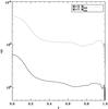Fig. 9 The product of density with thermal diffusivity as a function of the radius for our two stellar models.

The foregoing inequality is not very stringent: in the case that we are considering, only the slowly rotating models do not meet this inequality. This threshold means that if turbulence, as described by (38), exists, then the stress is large enough to remove baroclinic flows.

When the mass-loss rate decreases, however, there must be a threshold below which turbulence cannot be maintained. We surmise that this occurs when the angular momentum flux that characterizes the baroclinic flow equals the angular momentum loss of the star; hence $\begin{array}{ccc}\mathit{J̇}\mathrm{=}\frac{\mathrm{2}}{\mathrm{3}}\mathit{Ṁ}\mathrm{\Omega }{\mathit{R}}^{\mathrm{2}}\lesssim \mathrm{4}\mathit{\pi }{\mathit{R}}^{\mathrm{2}}{\mathit{V}}_{\mathit{r}}^{\mathrm{baroc}}\mathit{,}& & \end{array}$which also reads $\begin{array}{ccc}\mathit{Ṁ}\lesssim \mathit{Ṁ}\mathrm{c}\mathrm{=}\frac{\mathrm{3}\mathit{\pi }}{\mathrm{2}}\mathit{\mu R}{\left(\frac{\mathrm{𝒩}}{{\mathrm{\Omega }}_{\mathit{k}}}\right)}^{\mathrm{2}}\mathrm{·}& & \end{array}$We may compare this critical mass-loss rate to the transition one and we find $\mathit{Ṁ}\mathrm{c}\mathrm{~}\mathrm{4}\mathit{\lambda }{\left(\frac{\mathrm{𝒩}}{{\mathrm{\Omega }}_{\mathit{k}}}\right)}^{\mathrm{2}}\mathit{Ṁ}\mathit{t}\mathit{.}$(49)Since, for fast rotating models, λ ~ 2 × 10^-5, it turns out that Ṁ_c ~ 10^-3Ṁ_t for these stars, thus showing that a slight mass loss (~10^-11M_⊙/yr) may impose its dynamics on the stellar interior.

4.2. Spin-down by a rigid layer

We now turn to the other boundary condition where the spinning-down layer imposes its velocity. This case might represent a turbulent layer threaded by magnetic fields, which give some rigidity to the fluid. In these conditions, we can consider the case of Sect. 3.1. To further simplify the discussion, we assume that the layer is in a turbulent state triggered by internal shear and that buoyancy can be neglected so as to use the analytic solution (26).

The novelty introduced by these boundary conditions is that the transition from a baroclinic flow to the spin-down flow occurs in two steps. When the mass loss is increased, the meridional circulation first changes to that of the spin-down circulation. At a higher mass loss the differential rotation of baroclinic origin leaves the place to that of spin-down origin. The first threshold (meridional circulation) is reached when C_sd>E according to (32). With the help of (27), we find that this condition is equivalent to $\frac{\mathrm{5}\mathit{\beta }\mathrm{\left|}\mathit{Ṁ}\mathrm{\right|}\mathrm{\Omega }}{\mathrm{4}\mathit{\pi }{\mathit{R}}^{\mathrm{3}}\mathit{\rho }{\mathrm{𝒩}}^{\mathrm{2}}\mathit{\epsilon }}\mathit{>}\mathit{E}\mathit{.}$(50)In this expression β is arbitrary. As shown by (27), it is the parameter that connects the spin-down rate of the rigid layer and the mass-loss rate (or the angular momentum loss rate and Ṁ). Tentatively, we can estimate the product βṀ (or ) from (42) assuming high β. Then, inequality (50) leads to $\mathit{\lambda }\frac{\mathrm{3}{\mathrm{𝒩}}^{\mathrm{2}}{\mathit{R}}^{\mathrm{3}}}{\mathrm{5}\mathit{GM}}\mathit{<}\mathrm{1.}$(51)This new inequality is verified for fast rotating stars where λ ≪ 1 since $\frac{\mathrm{3}{\mathrm{𝒩}}^{\mathrm{2}}{\mathit{R}}^{\mathrm{3}}}{\mathrm{5}\mathit{GM}}\mathrm{~}\mathrm{10}$. This means that the meridional circulation is easily controlled by the spin-down process in fast rotating stars.

We shall not push the model further because we would clearly need a model for β namely for the relation between mass and angular momentum losses. We still note that criterion (51), as criterion (47), does not depend on the mass-loss rate, meaning that once the shear turbulence due to decelerating layers is settled, the baroclinic flows is replaced by the spin-down flow provided λ is small enough.

4.3. Comparison with previous estimates of Zahn (1992)

We may now compare our estimates of the amplitude of the circulation with the previous estimate of Zahn (1992). From his Eq. (4.15), he states that $\begin{array}{ccc}{\mathit{V}}_{\mathrm{mer}}^{\mathrm{Z}\mathrm{92}}\mathrm{\approx }\frac{\mathrm{15}}{\mathrm{8}\mathit{\pi }}\frac{\mathit{J̇}}{\mathit{\rho }{\mathit{R}}^{\mathrm{4}}\mathrm{\Omega }}\mathit{,}& & \end{array}$while our model with the rigid layer and β ≫ 1 says that $\begin{array}{ccc}{\mathit{V}}_{\mathrm{mer}}\mathrm{\simeq }\frac{\mathit{\epsilon }{\mathrm{𝒩}}^{\mathrm{2}}\mathit{R}}{\mathrm{2}\mathrm{\Omega }}{\mathit{C}}_{\mathrm{sd}}\mathrm{=}\frac{\mathrm{15}\mathit{J̇}}{\mathrm{16}\mathit{\pi \rho }\mathrm{\Omega }{\mathit{R}}^{\mathrm{4}}}\mathrm{·}& & \end{array}$Hence, up to an unimportant factor 2, the two expressions are identical. This is also the case for the stress-driven flow. Here,

$\begin{array}{ccc}{\mathit{V}}_{\mathrm{mer}}\mathrm{~}\frac{\mathit{\epsilon }{\mathrm{𝒩}}^{\mathrm{2}}\mathit{R}}{\mathrm{2}\mathrm{\Omega }}\mathit{E\tau }\mathrm{=}\frac{\mathrm{3}\mathit{J̇}}{\mathrm{16}\mathit{\pi \rho }\mathrm{\Omega }{\mathit{R}}^{\mathrm{4}}}& & \end{array}$where the two expressions are also of similar order of magnitude.

Zahn (1992) distinguishes two regimes for the mass loss: the strong wind and the moderate wind regimes. For Zahn the strong wind regime corresponds to an angular momentum loss timescale t_J shorter than k²t_ES, where k² is such that k²MR² is the moment of inertia of the star, and t_ES is the Eddington-Sweet timescale. Noting that and t_ES = t_KH/ε, the strong wind condition t_J<k²t_ES reads $\begin{array}{ccc}\frac{\mathit{J̇}}{\mathit{J}}\mathit{>}\frac{\mathit{\epsilon }}{{\mathit{k}}^{\mathrm{2}}{\mathit{t}}_{\mathrm{KH}}} \mathrm{or} \mathit{Ṁ}\mathit{>}\frac{\mathrm{3}\mathit{\epsilon M}}{\mathrm{2}{\mathit{t}}_{\mathrm{KH}}}\mathrm{=}\mathit{Ṁ}\begin{array}{c}\mathrm{Z}\mathrm{92}\\ \mathrm{c}\end{array}& & \end{array}$where t_KH is the Kelvin-Helmholtz timescale. Physically, Zahn’s critical mass-loss rate corresponds to the case where a circulation on the Eddington-Sweet time scale can no longer supply the wind with enough angular momentum.

This transition may be compared to our mass-loss rate where turbulence limits the extraction of angular momentum. We may therefore compare the two rates. We find that $\begin{array}{ccc}\mathit{Ṁ}\begin{array}{c}\mathrm{Z}\mathrm{92}\\ \mathrm{c}\end{array}\mathrm{=}\frac{\mathrm{3}}{\mathit{\pi }}\frac{\mathit{\epsilon }\mathrm{ℒ}}{\mathit{GM\rho \kappa }}{\left(\frac{\mathrm{𝒩}}{\mathrm{2}\mathrm{\Omega }}\right)}^{\mathrm{2}}\mathit{Ṁ}\mathit{t}& & \end{array}$where we used t_KH = 3GM²/ 4ℒR, ℒ being the luminosity of the star. A numerical evaluation of the ratio between these two mass-loss rates gives $\begin{array}{ccc}\mathit{Ṁ}\begin{array}{c}\mathrm{Z}\mathrm{92}\\ \mathrm{c}\end{array}\mathrm{~}\mathrm{30}\mathit{Ṁ}\mathit{t}\mathrm{·}& & \end{array}$Quite clearly, this mass-loss rate is in the regime of the advection dominated angular momentum transport as shown by (42) and our strong wind limit is lower than Zahn’s.

5. Summary and conclusions

Investigating the flows induced by mass loss in a rotating star brought us to a simple model where the star is represented by a ball of (almost) constant density fluid spun down either by a spinning down outer layer or by stresses applied to its surface. Both conditions are supplemented by an outward radial mass flux that mimics the expanding star. Since one open question about such stars is that of the transport of elements in their radiative region, the question about mass-losing rotating stars is how strong should this mass loss be to govern the rotational mixing that is otherwise triggered by baroclinic flows?

The first step towards an answer to this question is to understand the underlying fluid dynamics problem. This is the problem of a spin-down flow and, as the well-known spin-up flow much investigated in the sixties (Greenspan 1969; Pedlosky 1979; Duck & Foster 2001), it is a boundary driven flow. Velocity boundary conditions are unfortunately not well defined in a star: the spinning down layer, which feels the angular momentum loss, is part of the star and is likely thickening with time (Lignières et al. 1996). If we nevertheless define an interface between the star and this layer, interface conditions require the continuity of the velocity field and of the applied stress. In order to make the problem tractable we considered two idealized cases: In the first case, the layer is assumed to behave like a rigid shell that spins down and absorbs matter to feed the wind. That situation might describe a turbulent layer threaded by magnetic fields where magnetic fields provide some rigidity to an outer layer. The other idealized case assumes that the velocity field might be discontinuous at the interface but that the stresses are continuous. This condition is inspired by the ocean flows driven by wind stresses on our Earth.

This latter idealization turned out to be easier to deal with since it generalizes the results of Rieutord (2006a) in a simple way. It turns out that the baroclinic flows are overwhelmed by the spin-down flows when the non-dimensional stress is larger than unity. This simple change is due to the fact that both of these solutions (baroclinic and spin-down flows) meet boundary conditions on the stress (namely on the velocity derivatives).

The second case that we examined has a more complex behaviour. Here the velocity is prescribed at the interface. By writing the equations in a frame that co-rotates with the outer spinning-down layer, we can treat, at linear approximation, the spin-down flow and the baroclinic flow on an equal footing. When buoyancy can be neglected (needing a fast rotating star), an analytic solution of the spin-down flow may be derived.The main result is that as the forcing on spin-down increases, the transition from the baroclinic flow to the spin-down flow occurs in two steps: first, the meridional circulation transits to the spin-down circulation then the differential rotation does the same. The reason for that is that the baroclinic meridional circulation is of order of the Ekman number E (the non-dimensional measure of viscosity) compared to the associated differential rotation, while the spin-down meridional circulation is $\mathrm{𝒪}\mathrm{\left(}\sqrt{\mathit{E}}\mathrm{\right)}$ smaller than its associated differential rotation. Thus, when the baroclinic meridional circulation is replaced by the spin-down circulation, its differential rotation is still present.

These fluid dynamics results show that many thresholds might exist in terms of the spin-down drivings, or in terms of mass-loss rates.

Using the stress prescription, we could identify a transition mass-loss rate (Ṁ_t) that separates moderate wind regimes where the angular momentum flux is mainly realized through friction from a strong wind regime where angular momentum advection dominates. This peculiar mass-loss rate is determined by comparing advection of angular momentum and turbulent stresses that result from Zahn (1992) prescription together with the angular velocity profile associated with a constant specific angular momentum (Lignières et al. 1996). It turns out that this transition mass-loss rate reads $\mathit{Ṁ}\mathrm{t}\mathrm{=}\frac{\mathrm{2}\mathit{\pi }}{\mathrm{3}}\mathit{\rho \kappa R}{\left(\frac{\mathrm{2}\mathrm{\Omega }}{\mathrm{𝒩}}\right)}^{\mathrm{2}}\mathrm{·}$(52)For the two stellar models that we are using as test cases, we find that this mass-loss rate is 10^-8 and 4 × 10^-7 solar mass per year for a 3 M_⊙ and 7 M_⊙ ZAMS stars rotating rapidly (at 200 km s^-1 and 320 km s^-1 resp.). As shown by (52) this mass-loss rate decreases with rotation as Ω². For winds stronger or equal to the “transition” wind, the spin-down flow completely dominates over the baroclinic one. When the mass-loss rate decreases below Ṁ_t one may identify a threshold where the spin-down flow leaves the place to the baroclinic flows. This critical mass-loss rate is about three orders of magnitude less than Ṁ_t for the fast rotating stars that we are considering. Hence, the model where the spin-down is imposed via stresses at some boundary display three wind regimes:

• a weak wind case where the baroclinic flows dominate,

• a moderate wind case where spin-down flows have superseded baroclinic flows,

• a strong wind regime where angular momentum is essentially advected by the radial outflow.

The velocity prescription describing a rigid shell covering the star interior implies more restrictive conditions for the baroclinic flows to be superseded by the spin-down flows. The moderate wind threshold is the same as before, but at this strength the meridional circulation is the only part of the baroclinic flow that is changed. The mass-loss rate would need to be increased by a factor E^{− 1/2} for spin-down differential rotation to supersede the baroclinic differential rotation, but this conclusion is rather uncertain as it requires a modelling of the relation between mass and angular momentum losses.

We then compared these results with those of Zahn (1992) when this was possible. We found that his estimate of the meridional circulation in the case of a moderate wind well agreed with our estimates either with our rigid shell model or with the stress-driven spin-down. On the other hand, our estimate of the threshold for the strong wind regime is less by an order of magnitude than that of Zahn’s (for our two examples of stars). We understand this difference with the hypothesis underlying the two approaches. Zahn (1992) assumes a slow rotation where circulation is a transient flow independent of the viscosity, while ours is designed for fast rotating stars and uses steady solutions where viscosity plays a crucial role.

The reader may wonder how these results may apply to real stars where density is far from being constant. Compressibility is certainly one of the important improvements to make on such a modelling, however, time-dependence is likely as important especially in the strong wind regime. Finally, the interaction between the wind and the star is a process that requires more investigations. So the numerical estimates of some remarkable mass-loss rates, although reasonable, should not be taken at face value in view of the strong hypothesis that lead to them.

The important points of this work is rather the identification of the various mechanisms that may be at work when the angular momentum loss of a star is increased. We hope that this work will be a useful guide in the understanding of full-numerical multi-dimensional models of mass-losing rotating stars and that it clearly underscores the crucial points to be dealt with.

Acknowledgments

We are very grateful to Sylvie Théado for providing us with stellar models of ZAMS stars and to François Lignières for his remarks on an early version of the manuscript. We also thank the referee, Georges Meynet for his detailed and constructive criticism of the manuscript. We acknowledge support of the French Agence Nationale de la Recherche (ANR), under grant ESTER (ANR-09-BLAN-0140). This work was also supported by the Centre National de la Recherche Scientifique (C.N.R.S.), through the Programme National de Physique Stellaire (P.N.P.S.). The numerical calculations have been carried out on the CalMip machine of the “Centre Interuniversitaire de Calcul de Toulouse” (CICT) which is gratefully acknowledged.

References

All Tables

All Figures

	Fig. 1 Schematic view of the system: the spinning down turbulent envelope surrounds stably stratified fluid where the spin-down flow develops. The scale-filled outer cylinder of fractional radius s = cosα = 2/$\sqrt{\mathrm{7}}$ is an unstable region that may exist in some cases (see Sect. 3.1.3).
In the text

	Fig. 2 Adopted profile for the Brunt-Väisälä frequency in our calculations. We take the core radius at r = 0.15.
In the text

	Fig. 3 Comparison between the analytical (solid line) and numerical (+) solutions of the equatorial differential rotation of a spin-down flow (E = 10-6 and β = 3). s is the radial coordinate.
In the text

	Fig. 4 Meridional circulation associated with a spin-down flow in the case of Fig. 3. The dotted isocontours show a clockwise circulation, while the solid lines are for anti-clockwise circulation. Numerical resolution used Nr = 150 Chebyshev polynomials radially and spherical harmonics up to order L = 160.
In the text

Fig. 5 Differential rotation of a stably stratified rotating fluid in a sphere when the spin-down forcing Csd is strengthened. From left to right and top to bottom Csd = 0, − 10-6, − 10-5, − 10-4, − 10-3, − 10-2. Ekman and Prandtl numbers are E = 10-7, Pr = 10-4. All calculations have assumed β ≫ 1. Solid lines are for positive values, dotted for negative values. Numerical resolution used Nr = 200 Chebyshev polynomials radially and spherical harmonics up to order L = 250.

In the text

	Fig. 6 Meridional circulation in a stably stratified rotating fluid in a sphere when the spin-down forcing Csd is increased (Csd = 0,10-6,10-5from left to right). Streamlines of the meridional circulations are shown in the same way as in Fig. 4. As in Fig. 5, E = 10-7, Pr = 10-4, and β ≫ 1. Numerical resolution is the same as in Fig. 5.
In the text

Fig. 7 Differential rotation when the spin-down forcing Csd is strengthened while the buoyancy is influential. From left to right and top to bottom Csd = 0, − 10-6, − 10-5, − 10-4, − 10-3, − 10-2 We use E = 10-7, Pr = 3 × 10-2, $\mathit{\lambda }\mathrm{\simeq }\mathrm{3}\mathrm{\times }{\mathrm{10}}^{-2}\mathrm{=}\mathrm{100}\sqrt{\mathit{E}}$ and β ≫ 1. Top row: the flow is dominated by the baroclinic forcing. Bottom row: the flow is dominated by the spin-down forcing. Numerical resolution is the same as in Fig. 5.

In the text

	Fig. 8 Change in the meridional circulation when the spin-down forcing is increased. We represent the streamlines of the meridional circulation for Csd = 0,10-6,10-5from left to right. As in Fig. 7E = 10-7, Pr = 3 × 10-2 and β ≫ 1. Solid line show counter-clockwise circulation. Numerical resolution is the same as in Fig. 5.
In the text

	Fig. 9 The product of density with thermal diffusivity as a function of the radius for our two stellar models.
In the text

References

- Duck, P., & Foster, M. 2001, Ann. Rev. Fluid Mech., 33, 231 [Google Scholar]
- Espinosa Lara, F., & Rieutord, M. 2007, A&A, 470, 1013 [NASA ADS] [CrossRef] [EDP Sciences] [Google Scholar]
- EspinosaLara, F., & Rieutord, M. 2013, A&A, 552, A35 [NASA ADS] [CrossRef] [EDP Sciences] [Google Scholar]
- Friedlander, S. 1976, J. Fluid Mech., 76, 209 [NASA ADS] [CrossRef] [Google Scholar]
- Greenspan, H. P. 1969, The Theory of Rotating Fluids (Cambridge University Press) [Google Scholar]
- Hui-Bon-Hoa, A. 2008, Ast. Space Sc., 316, 55 [Google Scholar]
- Hypolite, D., & Rieutord, M. 2014, A&A, submitted [arXiv:1409.6129] [Google Scholar]
- Lau, H. H. B., Potter, A. T., & Tout, C. A. 2011, MNRAS, 415, 959 [NASA ADS] [CrossRef] [Google Scholar]
- Lignières, F., Catala, C., & Mangeney, A. 1996, A&A, 314, 465 [Google Scholar]
- Lignières, F., Catala, C., & Mangeney, A. 2000 [arXiv:astro-ph/0002026] [Google Scholar]
- Pedlosky, J. 1979, Geophysical fluid dynamics (Springer) [Google Scholar]
- Pinsonneault, M. 1997, ARA&A, 35, 557 [NASA ADS] [CrossRef] [Google Scholar]
- Rieutord, M. 1987, Geophys. Astrophys. Fluid Dyn., 39, 163 [Google Scholar]
- Rieutord, M. 1992, A&A, 259, 581 [Google Scholar]
- Rieutord, M. 2006a, A&A, 451, 1025 [NASA ADS] [CrossRef] [EDP Sciences] [Google Scholar]
- Rieutord, M. 2006b, in Stellar fluid dynamics and numerical simulations: From the sun to neutron stars, eds. M. Rieutord, & B. Dubrulle, 21, EAS, 275 [Google Scholar]
- Rieutord, M., & Espinosa Lara, F. 2013, in Lect. Notes Phys. (Berlin: Springer Verlag), 865, eds. M. Goupil, K. Belkacem, C. Neiner, F. Lignières, & J. J. Green, 49 [arXiv:1208.4926] [Google Scholar]
- Rieutord, M., & Zahn, J.-P. 1997, ApJ, 474, 760 [NASA ADS] [CrossRef] [Google Scholar]
- Turner, J. S. 1986, J. Fluid Mech., 173, 431 [NASA ADS] [CrossRef] [Google Scholar]
- von Zeipel, H. 1924, in Probleme der Astronomie (Festschrift für H. von Seeliger Springer), 144 [Google Scholar]
- Zahn, J.-P. 1992, A&A, 265, 115 [NASA ADS] [Google Scholar]