| Issue |
A&A
Volume 569, September 2014
|
|
|---|---|---|
| Article Number | A106 | |
| Number of page(s) | 21 | |
| Section | Stellar structure and evolution | |
| DOI | https://doi.org/10.1051/0004-6361/201424352 | |
| Published online | 30 September 2014 | |
Pulsating low-mass white dwarfs in the frame of new evolutionary sequences
I. Adiabatic properties
1 Grupo de Evolución Estelar y Pulsaciones. Facultad de Ciencias Astronómicas y Geofísicas, Universidad Nacional de La Plata, Paseo del Bosque s/n, 1900 La Plata, Argentina
2 IALP – CONICET, Argentina
e-mail: This email address is being protected from spambots. You need JavaScript enabled to view it.
, This email address is being protected from spambots. You need JavaScript enabled to view it.
Received: 6 June 2014
Accepted: 31 July 2014
Abstract
Context. Many low-mass white dwarfs with masses M∗/M⊙ ≲ 0.45, including the so-called extremely low-mass white dwarfs (M∗/M⊙ ≲ 0.20 − 0.25), have recently been discovered in the field of our Galaxy through dedicated photometric surveys. The subsequent discovery of pulsations in some of them has opened the unprecedented opportunity of probing the internal structure of these ancient stars.
Aims. We present a detailed adiabatic pulsational study of these stars based on full evolutionary sequences derived from binary star evolution computations. The main aim of this study is to provide a detailed theoretical basis of reference for interpreting present and future observations of variable low-mass white dwarfs.
Methods. Our pulsational analysis is based on a new set of He-core white-dwarf models with masses ranging from 0.1554 to 0.4352 M⊙ derived by computing the non-conservative evolution of a binary system consisting of an initially 1 M⊙ ZAMS star and a 1.4 M⊙ neutron star. We computed adiabatic radial (ℓ = 0) and non-radial (ℓ = 1,2) p and g modes to assess the dependence of the pulsational properties of these objects on stellar parameters such as the stellar mass and the effective temperature, as well as the effects of element diffusion.
Results. We found that for white dwarf models with masses below ~ 0.18 M⊙, g modes mainly probe the core regions and p modes the envelope, therefore pulsations offer the opportunity of constraining both the core and envelope chemical structure of these stars via asteroseismology. For models with M∗ ≳ 0.18 M⊙, on the other hand, g modes are very sensitive to the He/H compositional gradient and therefore can be used as a diagnostic tool for constraining the H envelope thickness. Because both types of objects have not only very distinct evolutionary histories (according to whether the progenitor stars have experienced CNO-flashes or not), but also have strongly different pulsation properties, we propose to define white dwarfs with masses below ~ 0.18 M⊙ as ELM (extremely low-mass) white dwarfs, and white dwarfs with M∗ ≳ 0.18 M⊙ as LM (low-mass) white dwarfs.
Key words: asteroseismology / stars: oscillations / white dwarfs / stars: evolution / stars: interiors / stars: variables: general
© ESO, 2014
1. Introduction
According to the current theory of stellar evolution, most low- and intermediate-mass (M∗ ≲ 11 M⊙; Siess 2007) stars that populate our Galaxy will end their lives as white dwarf (WD) stars. These old and compact stellar remnants have encrypted inside them a precious record of the evolutionary history of the progenitor stars, providing a wealth of information about the evolution of stars, star formation, and the age of a variety of stellar populations, such as our Galaxy and open and globular clusters (García-Berro et al. 2010; Althaus et al. 2010). Almost 80% of the WDs exhibit H-rich atmospheres; they define the spectral class of DA WDs. The mass distribution of DA WDs peaks at ~ 0.59 M⊙, and also exhibits high- and low-mass components (Kepler et al. 2007; Tremblay et al. 2011; Kleinman et al. 2013). The population of low-mass WDs has masses lower than 0.45 M⊙ and peaks at ~ 0.39 M⊙. In recent years, many low-mass WDs with M∗ ≲ 0.20−0.25 M⊙ have been detected through the ELM survey and the SPY and WASP surveys (see Koester et al. 2009; Brown et al. 2010, 2012; Maxted et al. 2011; Kilic et al. 2011, 2012); they are commonly referred to as extremely low-mass (ELM) WDs.
Low-mass WDs are probably produced by strong mass-loss episodes at the red giant branch (RGB) phase before the He-flash onset. Since the ignition of He is avoided, these WDs are expected to harbour He cores, in contrast to average mass WDs, which all probably contain C/O cores. For solar metallicity progenitors, mass-loss episodes must occur in binary systems through mass-transfer, since single-star evolution is not able to predict the formation of these stars in a Hubble time. This evolutionary scenario is confirmed by the fact that most of low-mass WDs are found in binary systems (e.g., Marsh et al. 1995), and usually as companions to millisecond pulsars (van Kerkwijk et al. 2005). In particular, binary evolution is the most likely origin for ELM WDs (Marsh et al. 1995). The evolution of low-mass WDs is strongly dependent on their stellar mass and the occurrence of element diffusion processes. Althaus et al. (2001) and Panei et al. (2007) have found that element diffusion leads to a dichotomy in the thickness of the H envelope, which translates into a dichotomy in the age of low-mass He-core WDs. Specifically, for stars with M∗ ≳ 0.18 − 0.20 M⊙, the WD progenitor experiences multiple diffusion-induced CNO thermonuclear flashes that engulf most of the H content of the envelope, and as a result, the remnant enters the final cooling track with a very thin H envelope. As a result, the star is unable to sustain stable nuclear burning while it cools, and the evolutionary timescale is rather short (~ 107 yr)1. On the other hand, if M∗ ≲ 0.18−0.20 M⊙, the WD progenitor does not experience H flashes at all, and the remnant enters its terminal cooling branch with a thick H envelope. This is thick enough for residual H nuclear burning to become the main energy source, which ultimately slows down the evolution, in which case the cooling timescale is of about ~ 109 yr. The age dichotomy has also been suggested by observations of the low-mass He-core WDs that are companions to millisecond pulsars (Bassa et al. 2003; Bassa 2006).
While some information such as surface chemical composition, temperature, and gravity of WDs can be inferred from spectroscopy, the internal structure of these compact stars can be unveiled only by means of asteroseismology, an approach based on the comparison between the observed pulsation periods of variable stars and appropriate theoretical models (Winget & Kepler 2008; Fontaine & Brassard 2008; Althaus et al. 2010). The first variable WD, HL Tau 76, was serendipitously discovered by Landolt (1968). Since then, many pulsating WDs have been detected. At present, there are several families of pulsating WDs known, which span a wide range in effective temperature and gravity (Fig. 1). Among them, the variables ZZ Ceti or DAVs (almost pure H atmospheres, 12 500 ≳ Teff ≳ 11 000 K) are the most numerous ones. The other classes comprise the DQVs (atmospheres rich in He and C, Teff ~ 20 000 K), the variables V777 Her or DBVs (atmospheres rich in He, 29 000 ≳ Teff ≳ 22 000 K), and the variables GW Vir (atmospheres dominated by C, O, and He) that include the DOVs and PNNVs objects (180 000 ≳ Teff ≳ 65 000 K). WD asteroseismology allows us to place constraints not only on global quantities such as gravity, effective temperature, or stellar mass, they provide, in addition, information about the thickness of the compositional layers, the core chemical composition, the internal rotation profile, the presence and strength of magnetic fields, the properties of the outer convective regions, and several other interesting properties (for a recent example in the context of ZZ Ceti stars, see Romero et al. 2012, 2013, and references therein).
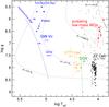 |
Fig. 1 Location of the several classes of pulsating WD stars in the log Teff − log g plane, marked with dots of different colours. In parenthesis we include the number of known members of each class. Two post-VLTP (Very Late Thermal Pulse) evolutionary tracks are plotted for reference. We also show the theoretical blue edge of the instability strip for the GW Vir stars, V777 Her stars, the DQV stars (Córsico et al. 2006, 2009a,b, respectively), the ZZ Ceti stars (Fontaine & Brassard 2008), and the pulsating low-mass WDs. For this last class, we show the blue edge according to Hermes et al. (2013a; dotted red line), Córsico et al. (2012; solid red line), and Steinfadt et al. (2010; dashed red line). For reference, we also include two evolutionary tracks of low-mass He-core white dwarfs from Althaus et al. (2013). Small black dots correspond to low-mass WDs that are non-variable or have not been observed yet to assess variability. |
The possible variability of low-mass WDs was first discussed by Steinfadt et al. (2010), who predicted that non-radial pulsation g modes with long periods should be excited in WDs with masses below ~ 0.2 M⊙. The various attempts to find pulsating objects of this type were unsuccessful, however (Steinfadt et al. 2012). This situation drastically changed with the exciting discovery of the first pulsating low-mass WD, SDSS J184037.78+642312.3, by Hermes et al. (2012). Subsequent searches resulted in the detection of two additional pulsating objects, SDSS J111215.82+111745.0 and SDSS J151826.68+065813.2 (Hermes et al. 2013b), and finally another two, SDSS J161431.28+191219.4 and SDSS J222859.93+362359.6 (Hermes et al. 2013a), all of them belonging to the DA spectral class and with masses below 0.24 M⊙. At present, this small group of five stars makes up a new, separate class of pulsating WDs. The effective temperatures of these stars are found to be between 10 000 K and 7800 K, which means that they are the coolest pulsating WDs known to date (see Fig. 1). Another distinctive feature of these stars is the length of their pulsation periods, Π ≳ 1180 s, longer than the periods found in ZZ Ceti stars (100 ≲ Π ≲ 1200 s). The period at Π = 6235 s detected in the power spectrum of SDSS J222859.93+362359.6 is the longest period ever measured in a pulsating WD star. On the other hand, SDSS J111215.82+111745.0 exhibits two short periods, at Π ~ 108 s and Π ~ 134 s, which might be caused by non-radial p modes or radial modes (ℓ = 0). If so, this would be the first detection of p or radial modes in a pulsating WD star. Finally, the existence of many non-variable stars in the region where pulsating objects are found (Fig. 1) suggests that the instability strip for low-mass WDs probably is not pure (Hermes et al. 2013a). This might be a hint that low-mass WDs that populate the same region in the log Teff − log g plane have substantially different internal structures and consequently quite different evolutionary origins.
Selected properties of our He-core WD sequences (final cooling branch) at Teff ≈ 10 000 K: the stellar mass, the mass of H in the outer envelope, the time it takes the star to cool from Teff ≈ 10 000 K to ≈ 8000 K, and the occurrence (or not) of CNO flashes on the early WD cooling branch.
The discovery of pulsating low-mass WDs constitutes a unique opportunity to probe the interiors of these stars and eventually to test their formation channels by employing the tools of asteroseismology. A first step in the theoretical study of these variable stars has been given by Córsico et al. (2012), who have thoroughly explored the g-mode adiabatic pulsation properties of the low-mass He-core WD models with masses in the range 0.17 − 0.46M∗ coming from high-metallicity progenitors (Z = 0.03) and single-star evolution computations. These authors also performed non-adiabatic pulsation computations and found many unstable g and p modes approximately at the correct effective temperatures and the correct range of the periods observed in pulsating low-mass WDs. This result has later been confirmed by Van Grootel et al. (2013).
To fully exploit the asteroseismological potential of this type of stars, accurate and realistic stellar models of low-mass WDs are crucial. To assess the correct thermo-mechanical structure of the WD and the thickness of the H envelope left by the pre-WD stage, the complete evolutionary history of the progenitor stars must be fully accounted for. A relevant physical ingredient that must be considered during the WD cooling phase is element diffusion to consistently account for the evolving shape of the internal chemical profiles (and, in particular, the chemical transition regions). Last but not least, stable H burning, which is particularly relevant in the case of ELM WDs (and might play a role in driving the pulsations), must be taken into account as well.
Motivated by the asteroseismological potential of pulsating low-mass WDs, and stimulated by the discovery of the first five variable objects of this type, we report a further step in the theoretical study of these stars by exploring the adiabatic pulsation properties of a new set of low-mass, He-core WD models with masses ranging from 0.1554 to 0.4352 M⊙ (including the mass range for ELM WDs, M∗/M⊙ ≲ 0.20−0.25, see Table 1) presented by Althaus et al. (2013), which were derived by computing the non-conservative evolution of a binary system consisting of an initially 1 M⊙ ZAMS star and a 1.4 M⊙ neutron star for various initial orbital periods. We here extend the study of Córsico et al. (2012) in two ways. First, we explore not only the non-radial g-mode pulsation spectrum of low-mas WD models, but we also study the non-radial p modes and the radial (ℓ = 0) pulsation spectrum. Second, thanks to the availability of five WD model sequences with progenitors that have not suffered from CNO-flashes (see Table 1), we are now able to explore the pulsation properties of ELM WDs in detail, which are characterised by very thick H envelopes. This is at variance with the work of Córsico et al. (2012), in which only one WD sequence (with mass M∗ = 0.17 M⊙) corresponded to a progenitor that did not experience H flashes. In this paper, we examine the possible differences in the pulsation properties of models with stellar masses near ~ 0.18−0.2 M⊙, which could be used as a seismic tool to distinguish stars that have undergone CNO flashes in their early-cooling phase from those that have not. We additionally discuss how our models match the observed properties of the known five pulsating low-mass WD stars. In particular, we determine whether our models are able to account for the short periods exhibited by SDSS J111215.82+111745.0 and evaluate the possibility that these modes might be p modes and/or radial modes. We also examine the hypothesis that one of these stars, SDSS J222859.93+362359.6, is not a genuine ELM WD, but instead a He pre-WD star undergoing a CNO flash episode. We defer to a second paper of this series a thorough non-adiabatic exploration of our complete set of He-core WD models.
The paper is organised as follows: In Sect. 2 we briefly describe our numerical tools and the main ingredients of the evolutionary sequences we use to assess the pulsation properties of low-mass He-core WDs. In Sect. 3 we present our pulsation results in detail. Section 4 is devoted to assessing how our models match the observations. Finally, in Sect. 5 we summarise our main findings.
2. Computational tools and evolutionary sequences
2.1. Evolutionary code and input physics
The evolutionary WD models employed in our pulsational analysis were generated with the evolutionary code LPCODE, which produces complete and detailed WD models that incorporate updated physical ingredients. While detailed information about LPCODE can be found in Althaus et al. (2005, 2009, 2013) and references therein, we list below only the ingredients employed that are relevant for our analysis of low-mass, He-core WD stars.
-
We adopted the standard mixing length theory (MLT) for convection (see, e.g., Kippenhahn et al. 2013) with the free parameter α = 1.6. With this value, the present luminosity and effective temperature of the Sun, log Teff = 3.7641 and L⊙ = 3.842 × 1033 erg s-1, at an age of 4570 Myr, are reproduced by LPCODE when Z = 0.0164 and X = 0.714 are adopted, in agreement with the Z/X value of Grevesse & Sauval (1998). A different convective efficiency that could change the temperature profiles of our models would have no direct impact on their adiabatic pulsation properties.
-
We assumed the metallicity of the progenitor stars to be Z = 0.01.
-
Radiative opacities for arbitrary metallicity in the range from 0 to 0.1 were taken from the OPAL project (Iglesias & Rogers 1996). At low temperatures, we used the updated molecular opacities with varying C/O ratios computed at Wichita State University (Ferguson et al. 2005) that were presented by Weiss & Ferguson (2009).
-
The conductive opacities were taken from Cassisi et al. (2007).
-
The equation of state during the main-sequence evolution is that of OPAL for a H- and He-rich composition.
-
Neutrino emission rates for pair, photo, and bremsstrahlung processes were taken from Itoh et al. (1996), and for plasma processes we included the treatment of Haft et al. (1994).
-
For the WD regime we employed an updated version of the Magni & Mazzitelli (1979) equation of state.
-
The nuclear network takes into account 16 elements and 34 thermonuclear reaction rates for pp-chains, CNO bi-cycle, He burning, and C ignition.
-
Time-dependent diffusion caused by gravitational settling and chemical and thermal diffusion of nuclear species was taken into account following the multi-component gas treatment of Burgers (1969).
-
Abundance changes were computed according to element diffusion, nuclear reactions, and convective mixing. This detailed treatment of abundance changes by different processes during the WD regime constitutes a key aspect in evaluating the importance of residual nuclear burning for the cooling of low-mass WDs.
-
For the WD regime and for effective temperatures lower than 10 000 K, outer boundary conditions for the evolving models were derived from non-grey model atmospheres (Rohrmann et al. 2012).
2.2. Pulsation codes
We carried out a detailed adiabatic radial (ℓ = 0) and non-radial p- and g-mode (ℓ = 1,2) pulsation analysis. The pulsation computations were performed with the adiabatic version of the pulsation code LP-PUL that is described in detail in Córsico & Althaus (2006), which is coupled to the LPCODE evolutionary code. The pulsation code is based on a general Newton-Raphson technique that solves the full fourth-order set of real equations and boundary conditions that govern linear, adiabatic, radial, and non-radial stellar pulsations following the dimensionless formulation of Dziembowski (1971) (see Unno et al. 1989). The prescription we followed to assess the run of the Brunt-Väisälä frequency (N) for a degenerate environment typical of the deep interior of a WD is the so-called Ledoux modified treatment (Tassoul et al. 1990). For our exploratory stability analysis described in Sect. 4.2, we employed the non-adiabatic version of the code LP-PUL described in Córsico et al. (2006). The code solves the full sixth-order complex system of linearised equations and boundary conditions as given by Unno et al. (1989). The caveat is that our non-adiabatic computations rely on the frozen-convection approximation, in which the perturbation of the convective flux is neglected. While this approximation is known to give unrealistic locations of the g-mode red edge of instability, it leads to satisfactory predictions for the location of the blue edge of the ZZ Ceti (DAV) instability strip (see, e.g., Brassard & Fontaine 1999; Van Grootel et al. 2012) and also for the V777 Her (DBV) instability strip (see, for instance, Beauchamp et al. 1999; Córsico et al. 2009a).
2.3. Evolutionary sequences
To derive realistic configurations for the low-mas He-core WDs, Althaus et al. (2013) mimicked the binary evolution of progenitor stars. Since H-shell burning is the main source of star luminosity during most of the evolution of ELM WDs, computating realistic initial WD structures is a fundamental requirement, in particular for correctly assessing the H-envelope mass left by progenitor evolution (see Sarna et al. 2000).
Binary evolution was assumed to be fully non-conservative, and the loss of angular momentum through mass loss, gravitational-wave radiation, and magnetic braking was considered. All of the He-core WD initial models were derived from evolutionary calculations for binary systems consisting of an evolving low-mass component of initially 1 M⊙ and a 1.4 M⊙ neutron star as the other component. Metallicity was assumed to be Z = 0.01. A total of 14 initial He-core WD models with stellar masses between 0.155 and 0.435 M⊙ were computed for initial orbital periods at the beginning of the Roche-lobe phase in the range 0.9 to 300 d. While full details about the procedure to obtain the initial models are provided in Althaus et al. (2013), we repeat here the prescriptions used by these authors to obtain the He-core WD models employed in this work. The formalism of Sarna et al. (2000) is followed. If M1 is the mass of the secondary (mass-losing) star, M2 the mass of the neutron star (primary), and Ṁ1 the mass-loss rate of the secondary, the change of the total orbital angular momentum (J) of the binary system can be written as 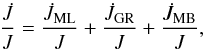 (1)where
  ,
,  , and
, and  are the angular momentum loss from the system through mass loss, gravitational-wave radiation, and magnetic braking (which is relevant when the secondary has an outer convection zone). To compute these quantities we follow Sarna et al. (2000) (see also Muslimov & Sarna 1993):
 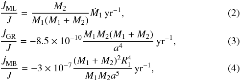 where a is the semi-axis of the orbit and R1 the radius of the secondary. All quantities are given in solar units. The mass-loss rate from the secondary is calculated as in Chen & Han (2002). Mass loss is considered as long as the secondary fills its Roche lobe rL, given by
 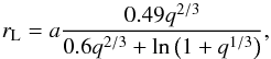 (5)where q = M1/M2 is the mass ratio. The semi-axis of the orbit is found by integrating the equation for the rate of change of a. If mass lost by the secondary is completely lost from the system, meaning that nothing of the mass lost by the secondary is accreted by the primary, a is given by (see Muslimov & Sarna 1993)
  (6)Mass loss is continued until the secondary star shrinks within its Roche lobe.
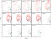 |
Fig. 2 log Teff − log g diagrams for the He-core WD sequences computed in Althaus et al. (2013). Sequences with masses in the range 0.18 ≲ M∗ ≲ 0.4 undergo CNO flashes during the early-cooling phase, which leads to the complex loops in the diagram. Green squares and magenta triangles correspond to the observed post-RGB low-mass stars from Silvotti et al. (2012) and Brown et al. (2013), and filled blue circles correspond to the five pulsating low-mass WDs detected so far (Hermes et al. 2013a). Numbers in the left upper corner of each panel correspond to the stellar mass at the WD stage. |
In Table 1, we provide some main characteristics of the whole set of He-core WD models. The evolution of these models was computed down to the range of luminosities of cool WDs, including the stages of multiple thermonuclear CNO flashes during the beginning of the cooling branch. The unstable H burning in CNO flashes occurs at the innermost tail of the H-abundance distribution. As the WD evolves along the cooling branch, chemical diffusion carries some H inwards to hotter and C-rich layers, where it burns unstably. In this region, the C abundance distribution is not modified by gravitational settling (Althaus et al. 2004). Column 1 of Table 1 shows the resulting final stellar masses (M∗/M⊙). The second column corresponds to the total amount of H contained in the envelope (MH/M∗) at Teff ≈ 10 000 K (at the final cooling branch), and Col. 3 displays the time spent by the models to cool from Teff ≈ 10 000 K to ≈ 8000 K. Finally, Col. 4 indicates the occurrence (or not) of CNO flashes on the early WD cooling branch. We note that, in good agreement with previous studies (Sarna et al. 2000; Althaus et al. 2001; Panei et al. 2007) there exists a threshold in the stellar mass value (at ~ 0.18 M⊙), below which CNO flashes on the early WD cooling branch are not expected to occur. Sequences with M∗ ≲ 0.18 M⊙ have thicker H envelopes and much longer cooling timescales than sequences with stellar masses above that threshold in mass. In numbers, this means that the H content is about four times higher and τ (the time to cool from Teff ≈ 10 000 K to Teff ≈ 8000 K) is about 22 times longer for the sequence with M∗ = 0.1762 M⊙ than for the sequence with M∗ = 0.1806 M⊙ (see Table 1). Note that in this example, we compare the properties of two sequences with virtually the same stellar mass (ΔM∗ ≈ 4 × 10⁻³ M⊙). The sequences without flashing evolve this slowly because the residual H-shell burning is the main source of surface luminosity, even at very advanced stages of evolution. It is clear that for these WDs, an appropriate treatment of progenitor evolution is required to correctly assess the evolutionary timescales. In contrast, an entirely different behaviour is expected for sequences that experience unstable H-shell burning on their early cooling branch. During the final cooling branch, evolution proceeds on a much shorter timescale than that characterising the sequences with M∗ ≲ 0.18 M⊙. This is because CNO flashes markedly reduce the H content of the star, with the result that residual nuclear burning is much less relevant when the remnant reaches the final cooling branch. The log Teff − log g diagrams for all the He-core WD sequences are shown in Fig. 2, which is an update of Fig. 2 of Althaus et al. (2013). Sequences that undergo CNO flashes during the early-cooling phase exhibit complex loops in the diagram. In contrast, sequences without flashes show very simple cooling tracks.
The mass limit below which low-mass WDs are classified as ELM WDs is not yet very clear in the literature. For instance, Brown et al. (2010, 2012, 2013) and Hermes et al. (2013b,a) defined low-mass WDs with M∗ ≲ 0.25 M⊙ as ELM WDs, while Kilic et al. (2011, 2012) classified objects with M∗ ≲ 0.20 M⊙as ELM WDs. Here, we propose to designate as ELM WDs those low-mass WDs that do not experience CNO flashes in their early-cooling branch. According to this classification, ELM WDs are low-mass WDs with masses below ~ 0.18 M⊙ in the frame of our computations2. This criterium is by no means arbitrary because both types of objects not only differ in their evolutionary history, but also show markedly different pulsation properties.
We conclude this section by showing in Fig. 3 the log Teff − log g plane in the region where pulsating low-mass WDs are found, along with the He-core low-mass WD evolutionary tracks of Althaus et al. (2013). Note that there is a gap between the two sets of tracks, corresponding to a stellar mass of ~ 0.18 M⊙. Interestingly, there are two pulsating stars, SDSS J184037.78+642312.3 and SDSS J111215.82+111745.0, which are located precisely in that transition region between ELM WDs and low-mass WDs, according to our definition. They are, therefore, very interesting targets for asteroseismology.
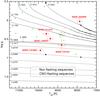 |
Fig. 3 Teff − log g plane showing the low-mass He-core WD evolutionary tracks of Althaus et al. (2013; thin black lines). Sequences with H flashes during the early-cooling phase are depicted with dashed lines, sequences without H flashes are displayed with solid lines. Numbers correspond to the stellar mass of each sequence. The locations of the five known pulsating low-mass WDs (Hermes et al. 2013a) are marked with a small circle (red). Stars not observed to vary are depicted with green triangles. Black circles and squares on the evolutionary tracks of M∗ = 0.1554 M⊙ and M∗ = 0.2389 M⊙ indicate the location of the template models analysed in Sect. 3.2. |
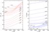 |
Fig. 4 Dipole (ℓ = 1) asymptotic period spacing of g modes (left panel) and the asymptotic frequency spacing of p modes (right panel) in terms of the effective temperature for all of our low-mass He-core evolutionary sequences. Dashed lines correspond to sequences with CNO flashes during the early-cooling phase, solid lines sequences without H flashes. |
3. Pulsation results
In this section we present the results of our detailed adiabatic survey of radial modes (ℓ = 0) and non-radial p and g modes (ℓ = 1,2) for the complete set of low-mass, He-core WD sequences of Althaus et al. (2013). We cover a wide range of effective temperatures (12 000 ≳ Teff ≳ 7000 K) and stellar masses (0.155 ≲ M∗/M⊙ ≲ 0.435). The set of the computed modes covers a very wide range of periods, embracing all the periodicities detected in pulsating low-mass WDs up to now. Specifically, the lower limit of the computed periods is between Πmin ~ 0.5 s (corresponding to M∗ = 0.4352 M⊙) and Πmin ~ 10 s (corresponding to M∗ = 0.1554 M⊙). They are associated with high-order radial modes and p modes, and were computed to account for the shortest periods detected in SDSS J111215.82+111745.0 (Π ~ 108 − 134 s). On the other hand, the upper limit of the computed periods (associated with high-order g modes) is Πmax ~ 7000 s, to account for the longest periods detected in SDSS J222859.93+362359.6 (Π ~ 6235 s).
In the next section we discuss our pulsational results by showing the predictions of the asymptotic theory of stellar pulsations.
3.1. Asymptotic period spacing (ΔΠa) and asymptotic frequency spacing (Δνa)
For g modes with high radial order k (long periods), the separation of consecutive periods (| Δk | = 1) becomes nearly constant at a value given by the asymptotic theory of non-radial stellar pulsations. Specifically, the asymptotic period spacing (Tassoul et al. 1990) is given by  (7)where
 ![Mathematical equation: \begin{equation} \label{asympeq} \Pi_0= 2 \pi^2 \left[\int_{r_1}^{r_2} \frac{N}{r} {\rm d}r\right]^{-1}. \end{equation}](/articles/aa/full_html/2014/09/aa24352-14/aa24352-14-eq108.png) (8)The squared Brunt-Väisälä frequency (N, one of the critical frequencies of non-radial stellar pulsations) is computed as
(8)The squared Brunt-Väisälä frequency (N, one of the critical frequencies of non-radial stellar pulsations) is computed as ![Mathematical equation: \begin{equation} N^2= \frac{g^2 \rho}{P}\frac{\chi_{T}}{\chi_{\rho}} \left[\nabla_{\rm ad}- \nabla + B\right], \label{bv} \end{equation}](/articles/aa/full_html/2014/09/aa24352-14/aa24352-14-eq109.png) (9)where the compressibilities are defined as
(9)where the compressibilities are defined as  (10)The Ledoux term B is computed as (Tassoul et al. 1990)
  (11)where
  (12)The expression in Eq. (7) is rigorously valid for chemically homogeneous stars. In this equation (see also Eq. (8)), the dependence of
  on the Brunt-Väisälä frequency is such that the asymptotic period spacing is larger when the mass and/or effective temperature of the model is lower. This trend is clearly visible in the left panel of Fig. 4, in which we depict the evolution of the asymptotic period spacing of g modes for all the sequences considered in this work. The higher values of for lower M∗ comes from the dependence N ∝ g, where g is the local gravity (
 ). On the other hand, the higher values of for lower Teff result from the dependence
  , with χT → 0 for increasing electronic degeneracy (T → 0). The abrupt change in the slope of the curves representing at certain effective temperatures (that decrease for decreasing stellar mass) is due to the appearance of surface convection in the models, which induces a lower value of the integral in Eq. (8) and the consequent increase of .
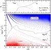 |
Fig. 5 Internal chemical profiles of He and H (upper panel) and the propagation diagram – the run of the logarithm of the squared critical frequencies (N, Lℓ) – (lower panel) corresponding to the ELM WD template model of M∗ = 0.1554 M⊙ and Teff ≈ 9600 K. Plus symbols (in red) correspond to the spatial location of the nodes of the radial eigenfunction of dipole (ℓ = 1) g modes, x symbols (in blue) represent the location of the nodes of dipole p modes. |
The strong dependence of the period spacing on M∗ shown in Fig. 4 might be used, in principle, to infer the stellar mass of pulsating low-mass WDs, provided that enough consecutive pulsation periods of g modes were detected. However, this prospect is severely complicated because the period spacing of pulsating WDs also depends on the thickness of the outer H envelope (Tassoul et al. 1990), being larger for thinner envelopes. This is particularly true in the context of low-mass He-core WDs, in which ELM WDs models, because of the absence of CNO flashes, harbour H envelopes that are several times thicker than more massive models. For the value of , and for a fixed Teff, therefore, a model with a low mass and a thick H envelope can readily mimic a more massive model with a thinner H envelope. A clear demonstration of this ambiguity can be found in Fig. 4, which shows a notorious degeneracy of the asymptotic period spacing. This figure shows for instance that for Teff ≳ 8500 K, ELM WD models with masses M∗ = 0.1762 M⊙ and M∗ = 0.1706 M⊙ have lower values of than the more massive models with M∗ = 0.1805 M⊙, which is caused by the much thicker H envelopes of the former models. If for a given pulsating star a rich spectrum of observed periods were available, this degeneracy might be broken by including additional information of the mode-trapping properties, which yield clues about the thickness of the H envelope.
The asymptotic frequency spacing of p modes (k ≫ 1), on the other hand, is given by (Unno et al. 1989) ![Mathematical equation: \begin{equation} \Delta \nu^{\rm a} = \left[2 \int_0^R \frac{{\rm d}r}{c_{\rm s}}\right]^{-1}, \label{afs} \end{equation}](/articles/aa/full_html/2014/09/aa24352-14/aa24352-14-eq128.png) (13)where cs is the local adiabatic sound speed, defined as
(13)where cs is the local adiabatic sound speed, defined as  . The asymptotic frequency spacing is related to the Lamb frequency (the other critical frequency of non-radial stellar pulsations) through cs by means of
 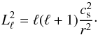 (14)In the right-hand panel of Fig. 4 we display the evolution of the asymptotic frequency spacing (in units of mHz ≡ 10-3 Hz) for all the sequences considered in this work. As can be seen, Δνa is larger for higher stellar masses and lower effective temperatures. This behaviour can be understood by realising that for higher M∗ and lower Teff, the values of the sound speed of the models globally increases, as a result of which the value of the integral in Eq. (13) is lower, and consequently, Δνa increases.
In contrast to what occurs for the for g modes, the asymptotic frequency spacing for p modes is not degenerate for sequences with CNO flashes (M∗ ≳ 0.18 M⊙) and those without (M∗ ≲ 0.18 M⊙, ELM WDs). This is because  is rather insensitive to the thickness of the H envelope. While an in-depth discussion of p modes in low-mass WDs is only of academic interest as yet, we can envisage that if these modes were confirmed in future observations, the eventual measurement of the mean frequency spacing for a real star might help in constraining its stellar mass.
3.2. Template models at the edges of the instability strip
To illustrate the adiabatic pulsation properties of our huge set of low-mass He-core WD models, which comprises more than 10 000 stellar structures, we focused on some selected, representative models. Since the instability domain of the known pulsating low-mass WDs in the log Teff − log g diagram is comprised between Teff ~ 10 000 K (the empirical blue edge) and Teff ~ 7800 K (the empirical red edge), we considered template models at both boundaries.
We first analyse two template models at Teff ~ 9600 K with stellar mass M∗ = 0.1554 M⊙ (ELM template model) and M∗ = 0.2389 M⊙ (LM template model). The ELM template model is representative of structures without CNO flashes in the past evolution (M∗ ≲ 0.18 M⊙), while the LM template model characterises the objects with H flashes (M∗ ≳ 0.18 M⊙). The location of these template models in the log Teff − log g diagram is indicated in Fig. 3 with black circles. Our models have a He core surrounded by a H outer envelope. In between, there is a smooth transition region shaped by the action of microscopic diffusion. In the upper panels of Figs. 5 and 6 we display the internal chemical profiles for He and H corresponding to the two template models. These template models are different in two important ways. To begin with, the ELM model has a H envelope that is about seven times thicker than the LM model. As mentioned, this is the result of the very different evolutionary history of the progenitor stars. Second, the He/H transition region is markedly wider for the ELM model than for the LM one. In particular, the H profile for the ELM model is characterised by a diffusion-shaped double-layered chemical structure, which consists of a pure H envelope on top of an intermediate remnant shell rich in H and He. We return to this in Sect. 3.4.
The chemical transition regions leave notorious signatures in the run of the squared critical frequencies, in particular in N. This is clearly displayed in the propagation diagrams(Cox 1980; Unno et al. 1989) of the lower panels in Figs. 5 and 6 that correspond to the template models. g modes propagate in the regions where  , and p modes in the regions where
  . Here, σ is the oscillation frequency. Note the very different shape of N2 for both models. In particular, one of the strongest differences is the location of the bump at the He/H transition region. Indeed, this bump is located at much deeper regions for the ELM model (r/R∗ ~ 0.2) than for the LM model (r/R∗ ~ 0.7). From the local maximum at r/R∗ ~ 0.22 (which coincides with the He/H transition region) outwards, N2 also decreases for the ELM model until it reaches a minimum at r/R∗ ~ 0.8. After that minimum, N2 reaches higher values in the surface layers. This is in contrast with the LM template model, in which the squared Brunt-Väisälä frequency exhibits higher values at the outer layers than at the core, which resembles the situation in the C/O core DAV WD models (see Fig. 3 of Romero et al. 2012). This notoriously different shape of the run of N2 has strong consequences for the propagation properties of eigenmodes. Specifically, and because of the particular shape of N2, which is larger in the core than in the envelope (see also Fig. 3 of Córsico et al. 2012), the resonant cavity of g modes for the ELM model is circumscribed to the core regions (r/R∗ ≲ 0.25) and the opposite holds for p modes, whereas for the LM model the propagation region for both g and p modes extends roughly along the whole model. To summarise, g modes in ELM WD models (M∗ ≲ 0.18 M⊙) mainly probe the core regions and p modes the envelope. This means that we have the opportunity to constrain both the core and envelope chemical structure of these stars via asteroseismology. Steinfadt et al. (2010) were the first to notice this important characteristic.
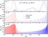 |
Fig. 7 Run of the density of kinetic energy dEekin/dr (normalised to 1) for radial modes (dashed blue) and dipole g (red) and p modes (solid blue curves) with k = 1 (upper panel), k = 10 (middle panel), and k = 60 (lower panel), corresponding to the ELM template model with M∗ = 0.1554 M⊙. The vertical dashed line marks the location of the He/H chemical transition region. |
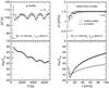 |
Fig. 9 ℓ = 1 forward period-spacing of g modes versus periods (upper left-hand panel), and the forward frequency-spacing of radial modes (hollow small circles) and p modes (filled small circles) versus frequencies (upper right-hand panel) and the associated oscillation kinetic energy distributions (lower panels) for the ELM WD template model with M∗ = 0.1554 M⊙ and Teff ~ 9600 K. The red horizontal lines in the upper panels correspond to the asymptotic period-spacing (left), computed with Eq. (7), and the asymptotic frequency-spacing (right), computed with Eq. (13). |
The property described above is vividly illustrated in Fig. 7, in which we display the density of the oscillation kinetic energy dEkin/dr, (see Appendix A of Córsico & Althaus 2006, for its definition) for radial modes, p and g modes with radial order k = 1,10, and 60 for the same ELM template model as was analysed in Fig. 5. It is apparent that most of the kinetic energy of g modes is confined to the regions below the He/H interface, meaning that most of the spatial oscillations are located in the region with r/R∗ ≲ 0.25. In contrast, the kinetic energy of p modes and radial modes is spread throughout the star, but concentrated more towards the surface regions and almost absent from the core.
In Fig. 8 we show the situation for the LM WD template model. At variance with the ELM model, there is no such a clear distinction in the behaviour of g modes with respect to p and radial modes. Indeed, the kinetic energy of g modes is spread throughout the model, although it is particularly concentrated in the region of the He/H interface and also at the surface. In this sense, low-mass He-core WDs with M∗ ≳ 0.18 M⊙ behave in a qualitative similar way as their massive cousins, the C/O-core DAV WD stars. p and radial modes are insensitive to the presence of the chemical interface because their kinetic energy is enhanced at the stellar surface. In summary, it is apparent that for LM WD models, g modes are very sensitive to the He/H compositional gradient and therfore can be a diagnostic tool to constrain the H envelope thickness of low-mass WD models with M∗ ≳ 0.18 M⊙.
We now examine the mode-trapping properties of our template models. Mode trapping of g modes is a well-studied mechanical resonance that acts in WD stars through chemical composition gradients. This means that one or more narrow regions in which the abundances of nuclear species (and consequently, the average molecular weight μ) vary spatially modify the character of the resonant cavity in which modes should propagate as standing waves. Specifically, chemical transition regions act like reflecting walls that partially trap certain modes, forcing them to oscillate with larger amplitudes in specific regions and with smaller amplitudes outside of those regions (see, for details, Brassard et al. 1992; Bradley et al. 1993; Córsico et al. 2002a). Mode trapping translates into local maxima and minima in Ekin, which are usually associated with modes that are partially confined to the core regions and modes that are partially trapped in the envelope. Unfortunately, the kinetic oscillation energy is hard to estimate from observations alone. A more important signature, which in principle can be employed as an observational diagnostic of mode trapping – provided that a series of periods with the same ℓ and consecutive radial order k is detected – is the strong departure from uniform period spacing, ΔΠ (≡Πk + 1 − Πk), when plotted in terms of the pulsation period Πk. For stellar models characterised by a single chemical interface, like those we consider here, local minima in ΔΠk usually correspond to modes trapped in the H envelope, whereas local maxima in ΔΠk are associated with modes trapped in the core region.
In the upper left-hand panel of Fig. 9 we show the dipole forward period-spacing of g modes versus periods for the ELM template model with M∗ = 0.1554 M⊙ and Teff ~ 9600 K. The upper right-hand panel corresponds to the forward frequency-spacing, Δν (≡νk + 1 − νk), of radial modes and p modes in terms of the frequency (in mHz) for the same model. Finally, the lower panels depict the kinetic energy distributions. For periods longer than about 1000 s, the period-spacing distribution of g modes shows a regular pattern of mode trapping with a very short trapping cycle (period interval between two trapped modes) of ~ 100 s and amplitude, superimposed on a high-amplitude variation characterised by a long trapping cycle (~ 1800 s). The simultaneous presence of these two patterns is the result of the double-layered chemical structure of the H profile that characterises the ELM WD template model at that effective temperature. This double-layered structure becomes a single-layered one by the action of element diffusion (see Sect. 3.4). The period spacing does not reach the asymptotic value in the period interval shown in the figure. The Ekin distribution only shows the long-trapping cycle pattern. We examined the radial eigenfunctions of two modes, one of them with k = 29 and associated to a local minimum of Ekin, and the other one with k = 33, corresponding to a maximum Ekin value. We realised that the eigenfunction of the k = 33 mode has larger amplitudes at the core regions than the k = 29 mode. It is apparent that as a general rule, all the g modes in the ELM WD template model are confined to the core regions, but some of them have eigenfunctions with larger amplitudes than the remaining ones. They correspond to local maxima in the Ekin distribution. On the other hand, the frequency spacing of radial modes and p modes are close to the asymptotic value for radial order k ≤ 9 and k ≤ 16, respectively. In this case, no mode-trapping signatures are visible in the kinetic energy distribution of the modes.
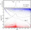 |
Fig. 11 Chemical profiles of He and H (upper panel) and the propagation diagram (lower panel) for the ELM WD template model of M∗ = 0.1554 M⊙ and Teff ≈ 7800 K. |
The results for the LM WD template model with M∗ = 0.2389 M⊙ and Teff ~ 9600 K are depicted in Fig. 10. For g modes, mode-trapping signatures are quite evident, but the trapping cycle (~ 200 s) of the present pattern is much shorter than for the high-amplitude variation of the ELM WD template model. Mode-trapping features are absent from the Ekin distribution, which instead is very smooth. Note that the ΔΠ values approach to the asymptotic prediction for periods longer than ~ 4000 s. The frequency separations of radial modes and p modes, on the other hand, show some signatures of mode trapping for low-order modes, and do not reach the asymptotic value for the range of frequencies considered in the plot.
We now describe the results for template models located at an effective temperature close to the Teff of the coolest known pulsating low-mass WD (SDSS J222859.93+362359.6, Teff = 7870 ± 120 K), which defines the empirical red edge of the instability strip of this new kind of variable stars. Specifically, we analyse two template models at Teff ~ 7800 K, one of them with a stellar mass M∗ = 0.1554 M⊙, and the other one with M∗ = 0.2389 M⊙. The location of these template models in the log Teff − log g plane is shown in Fig. 3 with black squares. In Figs. 11 and 12 we show their chemical profiles (upper panels) and propagation diagrams (lower panels). For the ELM template model, the changes in the chemical profiles caused by element diffusion while the star cools from Teff ~ 9600 K to Teff ~ 7800 are very noticeable. The shape of the He/H interface has changed from a double-layered to a single-layered structure (see Sect. 3.4). At this lower Teff the He/H transition is located at r/R∗ ~ 0.45 and results in a more external bump of the Brunt-Väisälä frequency than in the model at Teff ~ 9600 K (compare with Fig. 5). For the LM WD template model, the changes in the He/H chemical transition region and in the Brunt-Väisälä frequency due to element diffusion are less noticeable. When we compare the upper panels of Figs. 12 and 6, we barely note a slight variation in the thickness of the He/H transition region, which is somewhat narrow for the cooler model. This results in a slightly more narrow bump in the profile of N2.
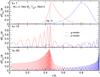 |
Fig. 13 Run of the density of kinetic energy dEekin/dr (normalised to 1) for dipole g (red) and p modes (solid blue curves) with k = 1 (upper panel), k = 10 (middle panel), and k = 60 (lower panel), for the ELM template model with M∗ = 0.1554 M⊙ and Teff ≈ 7800 K (analysed in Fig.11). |
In Figs. 13 and 14 we show dEkin/dr for p and g modes3 with k = 1,10, and 60 for the ELM and the LM template models at Teff ~ 7800 K. For the ELM model there is a clear distinction between p and g modes for the part of the star that they probe: g modes are mostly confined to the core, p modes to the envelope. The situation is therefore the same as for the ELM WD template model at Teff ~ 9600 K (see Fig. 7). A similar situation is found for the LM template model. At Teff ~ 7800 the g modes are very sensitive to the presence of the He/H transition region, whereas p modes (and radial modes, not shown) are concentrated towards the stellar surface and are unaffected by the presence of that chemical interface.
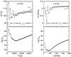 |
Fig. 15 ℓ = 1 forward period-spacing of g modes versus periods (upper left-hand panel), and the forward frequency-spacing of radial modes (hollow small circles) and p modes (filled small circles) versus frequencies (upper right-hand panel) and the corresponding kinetic energy distributions (lower panels) for the ELM WD template model with M∗ = 0.1554 M⊙ and Teff ~ 7800 K. |
Finally, in Figs. 15 and 16 we show the distributions of ΔΠ (g modes), Δν (p modes), and log (Ekin) for the ELM and the LM WD template models at Teff ≈ 7800 K. It is evident that the period-spacing pattern of g modes of the ELM template model at this low effective temperature is completely different from that for the ELM model at high Teff. Although the asymptotic period-spacing (and consequently, the average period-spacing) has not changed much, the ΔΠ distribution exhibits only a single signal of mode trapping, characterised by a short trapping cycle. Moreover, at variance with the model at Teff ≈ 9600 K, ΔΠ reaches the asymptotic value for Π ≳ 4000 s. The very distinct pattern of ΔΠ in comparison with the hot ELM template model is due to the strong differences in the chemical profiles, and ultimately in the run of the Brunt-Väisälä frequency (compare Figs. 5 and 11). The frequency-spacing pattern for Teff ~ 7800 K of the p modes (and radial modes, not shown) is similar to that found for Teff ~ 9600 K, but there is a strong difference in the asymptotic frequency-spacing (and thus, in the average frequency-spacing). In fact, Δνa = 4.16 mHz for the cool model is about three times larger than for the hot model (Δνa = 1.51 mHz). This marked difference originates in the fact that for the model at Teff ~ 7800 K the Lamb frequency adopts much higher values than for the model at Teff ~ 9600 K, and in turn, the integral in Eq. (13) is lower, and consequently, Δν is higher.
We did not find substantial differences in the patterns of ΔΠ and Δν (Fig. 16) in the LM WD template model compared with the hot template model (Fig. 10). For the cool template model, both ΔΠa and Δνa, and in turn the average ΔΠ and Δν, are larger than for the hot template model, however. This is a direct consequence of the decrease in the Brunt-Väisälä frequency and the increase in the Lamb frequency for decreasing effective temperatures. This behaviour was anticipated in Sect. 4 where we discussed the dependence of ΔΠa and Δνa on the effective temperature.
3.3. Effects of the total mass and the effective temperature
The period spacing and the periods themselves of g modes vary as the inverse of the Brunt-Väisälä frequency (see Sect. 3.1). The Brunt-Väisälä frequency, in turn, increases with higher stellar masses and with higher effective temperatures. As a result, the pulsation periods of g modes are longer for smaller mass (lower gravity) and lower effective temperature (increasing degeneracy). For p-modes and radial modes the sound speed decreases for lower M∗ and higher Teff, and consequently, the periods increase. We study the effects of M∗ and Teff separately below.
The effects of the stellar mass on the pulsation periods is shown in Fig. 17, where we plot Π for non-radial ℓ = 1g modes and p modes, and also for radial modes (ℓ = 0) in terms of M∗ for a fixed value of Teff = 9500 K. The periods of the three types of eigenmodes increase with decreasing stellar mass, as expected. The period gap that separates the families of p modes/radial modes and g modes notoriously shrinks for ELM WD models. The striking step in the run of the periods in terms of the mass is associated with the limit stellar mass value, at ~ 0.18 M⊙. Note the strong increase of the p- and radial-mode periods for ELM WDs (M∗ ≲ 0.18 M⊙). As can be seen, the period of the fundamental radial mode (r0) is substantially longer than the period corresponding to the k = 1p mode (p1) for LM WDs (M∗ ≳ 0.18 M⊙), but both periods adopt virtually the same values (as do other low-order pairs of modes, as well: r1–p2, r2–p3, etc.) for ELM WD models. Figure 18 displays the results for g, f and p modes with ℓ = 2. In this case, the g- mode periods are substantially shorter than ℓ = 1, and the branches of g and p modes are clearly split by the period of the f mode.
In summary, the deep structural differences between LM and ELM WD models are clearly illustrated by the very different behaviour of the periods (in particular of p modes and radial modes), as documented in Figs. 17 and 18.
In Fig. 19 we show the evolution of the pulsation periods of ℓ = 1g and p modes, and also radial modes with Teff for models with M∗ = 0.1917 M⊙. The lengthening of g-mode periods with decreasing effective temperature is evident, although the effect is much weaker than the decrease with the stellar mass (compare with Fig. 17). The p- and radial-mode periods, on the other hand, decrease with decreasing Teff.
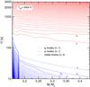 |
Fig. 17 Pulsation periods of ℓ = 1g- and p modes and also radial modes (ℓ = 0) in terms of the stellar mass for Teff = 9500 K. Periods increase with decreasing M∗. |
3.4. Effects of element diffusion
Here, we describe the effects of the evolving chemical profiles on the pulsation properties of low-mass, He-core WDs. This matter has been extensively explored in previous papers (see Córsico et al. 2002b, in the context of DAV stars). Time-dependent element diffusion strongly modifies the shape of the He and H chemical profiles as the WD cools, causing H to float to the surface and He to sink down. In particular, diffusion not only modifies the chemical composition of the outer layers, but also the shape of the He/H chemical transition region itself. This is clearly documented in Fig. 20 for the 0.1554 M⊙ ELM sequence in the Teff interval (9600−8000 K). For the model at Teff = 9600 K, the H profile is characterised by a diffusion-shaped double-layered chemical structure, which consists of a pure H envelope on top of an intermediate remnant shell rich in H and He. This structure still remains, although to a much weaker extent, in the model at Teff = 9000 K. Finally, from Teff ~ 8040 K down, the H profile adopts a single-layered chemical structure. This type of transitions of the shape of chemical profiles caused by element diffusion has previously been studied in detail in DB WDs (see, e.g., Althaus & Córsico 2004). Element diffusion processes affect all the sequences considered in this paper, although the transition from a double-layered to a single-layered structure occurs at different effective temperatures. The low surface gravity that characterises the model shown in Fig. 20 (log g ~ 5.5−6.2), which results in a weak impact of gravitational settling, and the very long timescale that characterises element diffusion processes at the depth where the He/H interface is located (r/R∗ ~ 0.2), eventually lead to a wider chemical transition than for more massive models. Because of this, the sequences with larger masses (M∗ ≳ 0.19 M⊙) reach the single-layered configuration at effective temperatures higher than ~ 10 000 K, beyond the domain in which pulsating objects are currently found.
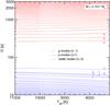 |
Fig. 19 Pulsation periods of ℓ = 1g modes and p modes/radial modes in terms of the effective temperature for M∗ = 0.1917 M⊙. g-mode periods increase with decreasing Teff; the opposite holds for p modes and radial modes. |
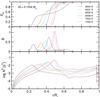 |
Fig. 20 Internal chemical profile of H (upper panel), the Ledoux term B entering in the computation of the Brunt-Väisälä frequency (see Eq. (11)) (middle panel), and the logarithm of the squared Brunt-Väisälä frequency (lower panel), for an ELM WD model with M∗ = 0.1554 M⊙ at different effective temperatures, as indicated. |
The evolution of the shape of the He/H chemical transition region are translated into noticeable changes in the run of the Brunt-Väisälä frequency (lower panel of Fig. 20), as a result of the changing Ledoux term B (middle panel of Fig. 20). In fact, at high effective temperatures, N2 is characterised by two bumps (the most prominent one located at r/R∗ ~ 0.25 and the smaller at r/R∗ ~ 0.62), which merge into a single bump (at r/R∗ ~ 0.5) when the chemical interface He/H adopts a single-layered structure. As was first emphasised by Córsico et al. (2012), and in the light of our results, diffusive equilibrium is not a valid assumption in the He/H transition region for ELM WD stars. Exploratory computations without element diffusion result in changes of up to 5% in the value of the periods compared with computations with element diffusion.
The effects of element diffusion for a more massive model (an LM WD model with M∗ = 0.2389 M⊙) at the same range of effective temperatures is less impressive, as is shown in Fig. 21. In this case, the H chemical profile does not change dramatically, and the same occurs with B and the Brunt-Väisälä frequency. Even so, this slight evolution in the shape of the chemical profiles is translated into non-negligible changes in the pulsation periods. Again, for LM WD stars it is necessary to properly account for element diffusion processes to accurately compute the period spectrum.
3.5. Template models with M∗ near the threshold mass
It is interesting to examine the pulsation properties of low-mass WD sequences with stellar masses near the critical mass for the development of CNO flashes (M ~ 0.18 M⊙). This is because at least three of the five ELM pulsating WDs reported by Hermes et al. (2013a) have stellar masses near this threshold value (see Fig. 3). Therefore it might be quite important to find an asteroseismic prospect to distinguish ELM from LM WDs (Althaus et al. 2013). Specifically, we focus on the most massive ELM WD sequence (M∗ = 0.1762 M⊙), and the lowest mass LM WD sequence (M∗ = 0.1805 M⊙). In Figs. 22 and 23 we display the chemical profiles (upper panels) and the propagation diagrams (central panels) for two models at Teff ~ 10 000 K. Interestingly enough, the H content and the shape of the chemical interface of He/H are very different even though the difference in the stellar mass of these two models is almost negligible: ΔM∗ = 0.0043 M⊙. The differences in the shape and location of the He/H interface (by virtue of the different thicknesses of the H envelope) for both models are translated into distinct features in the run of the squared critical frequencies, in particular in the Brunt-Väisälä frequency (middle panels). Note, in particular, the presence of two bumps in N2 in the LM model with M∗ = 0.1805 M⊙, which result from a double-layered chemical structure at the He/H interface. It differs from the single bump of N2 for the ELM model with M∗ = 0.1762 M⊙, which results from the single-layered shape of the He/H chemical transition region.
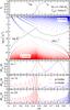 |
Fig. 22 Chemical profiles of He and H (upper panel), the propagation diagram (centre panel), and the kinetic energy density for dipole g (red) and p modes (solid blue curves) with k = 1,10, and 20 (lower panels), for an ELM WD model with M∗ = 0.1762 M⊙ and Teff ≈ 10 000 K. |
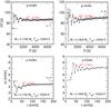 |
Fig. 24 Upper panels: ℓ = 1 forward period-spacing of g modes vs. periods. Lower panels: forward frequency-spacing of p modes vs. frequency. Left-hand panels: ELM WD model with M∗ = 0.1762 M⊙. Right-hand panels: LM WD model with M∗ = 0.1805 M⊙, both at Teff ~ 10 000 K. Red dashed lines correspond to the asymptotic predictions. |
The consequences of these differences are clearly illustrated in the propagation characteristics of the pulsation modes. The lower panels of Figs. 22 and 23 display the kinetic energy density of pulsation for ℓ = 1g and p modes with k = 1,10, and 20. As we found in Sect. 3.2, for the ELM WD model g modes are confined to the He core, and p modes have most of their kinetic energy located at the surface regions (Fig. 22). For g modes in the LM WD model, the kinetic energy is distributed throughout the model, and they are sensitive to the presence of the He/H interface. p modes, on the other hand, are rather insensitive to the chemical gradient and have most of their kinetic energy placed at the stellar surface (Fig. 23).
In Fig. 24 we show the forward period-spacing in terms of the dipole g-mode periods (upper panels) and the forward frequency-spacing in terms of the dipole p mode frequencies (lower panels) for the ELM WD template model with M∗ = 0.1762 M⊙ (left) and the LM WD template model with M∗ = 0.1805 M⊙ (right), the same models as considered in Figs. 22 and 23. Mode-trapping features in the form of strong departures of uniform period-spacing of g modes can be appreciated in both models, in particular for periods shorter than about 2000 s for the ELM WD model, and Π ≲ 4000 s for the LM WD model. Longer periods approach the asymptotic period-spacings, although even with low-amplitude deviations because of mode trapping. For periods shorter than ~ 3000 s, the amplitudes of deviations from a constant period separation are markedly larger for the LM than for the ELM model. In principle, this difference might be considered as a practical tool for distinguishing stars with CNO flashes in their early-cooling phase from those without, provided that enough consecutive low- and intermediate-order g modes with the same harmonic degree were observed in pulsating low-mass WDs (Althaus et al. 2013). This optimistic view is somewhat dampened because the most useful low radial-order g modes are most likely pulsationally stable, as shown from the non-adiabatic analysis of Córsico et al. (2012) and demonstrated by most of the observed pulsating low-mass WD stars, in which no periods shorter than about 1400 s are seen.
Finally, as for the p-modes, there are clear non-uniformities in the frequency spacing distributions, which are of similar amplitudes in both WD models. However, the asymptotic frequency-spacing for the LM WD model is about twice that for the ELM WD model, even though the difference in stellar mass is only ~ 0.004 M⊙. This strong difference in the mean frequency-spacing could also be exploited to distinguish between the two types of objects. To be able to employ this property as a useful seismological tool, however, it will be necessary to detect many p mode consecutive periods in pulsating low-mass WDs. At present, only a few short periods (Π ~ 108 − 134 s) have been detected in only one low-mass pulsating WD (SDSS J111215.82+111745.0), and still it remains to be determined whether they are genuine p modes or not (see Sect. 4.1 ). Thus, this potential asteroseismological tool is for now only of academic interest.
4. Interpretation of observations
Until today, five pulsating low-mass WD stars have been detected: SDSS J184037.78+642312.3 (Hermes et al. 2012), SDSS J111215.82+111745.0, SDSS J151826.68+065813.2 (Hermes et al. 2013b), SDSS J161431.28+191219.4, and SDSS J222859.93+362359.6 (Hermes et al. 2013a). They have very long pulsation periods, from ~ 1180 s up to ~ 6240 s, although one object (SDSS J111215.82+111745.0) also has short-period pulsations (108−134 s). Table 4 of Hermes et al. (2013a) lists the main properties of the five known pulsating low-mass WDs. These authors discuss the common properties of this set of pulsators at some length. In Fig. 3 we display the location of the stars in the log Teff − log g diagram, while in Figs. 25 and 26 we show the period spectrum of these pulsating stars in terms of the effective temperature and surface gravity. The long-period pulsations are most likely the result of intermediate- and high-order g modes (12 ≲ k ≲ 50 for ℓ = 1) excited by the κ − γ-mechanism that acts in the H partial ionisation zone, as indicated by stability computations (Córsico et al. 2012; Van Grootel et al. 2013). On the other hand, the short periods detected in SDSS J111215.82+111745.0 might be caused by p modes or even radial modes of low radial order, as was suggested by stability computations, although the precise nature of these periodicities still remains to be defined4.
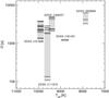 |
Fig. 25 Pulsation periods of the five known pulsating low-mass WD stars in terms of the effective temperature, according to Table 4 of Hermes et al. (2013a). |
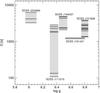 |
Fig. 26 Pulsation periods of the five known pulsating low-mass WD stars in terms of the surface gravity, according to Table 4 of Hermes et al. (2013a). |
Although there are very few objects currently available to establish any trend, Figs. 25 and 26 reveal a certain correlation of the long periods (those presumably associated with g modes) with g and Teff. Specifically, periods are longer for lower gravities and effective temperatures. These trends are expected from theoretical grounds, as discussed by Hermes et al. (2013a). For instance, in the context of the κ − γ-mechanism of mode driving, the trend of the periods to be longer for cooler stars is related to the fact that the outer convection zone in a WD star deepens with cooling, with the consequent increase in the thermal timescale (τth) at its base. Since the periods of the excited modes are of the order of τth, modes with increasingly longer periods are gradually excited as the WD cools. This is an often-studied property of ZZ Ceti stars (Mukadam et al. 2006)5. Similarly, the trend of periods with gravity (and thus, with M∗) can be understood by realising that lower g imply lower mean densities (ρ), and that the pulsation periods roughly scale with the dynamical timescale for the whole star, Π ∝ ρ1/2 (Hermes et al. 2013a).
We emphasise that while these arguments qualitatively explain the trends observed in the period spectrum of the five known pulsating low-mass WDs, the final decision on this matter relies on detailed non-adiabatic pulsation calculations like those performed by Córsico et al. (2012) and Van Grootel et al. (2013). We defer a complete and detailed study of the non-adiabatic pulsation properties of our set of low-mass He-core WD models to a forthcoming paper. In the next two sections, we interpret the short periods in SDSS J111215.82+111745.0 by considering adiabatic periods alone (Sect. 4.1), and the possibility that SDSS J222859.93+362359.6 is a pre-WD star instead of a genuine ELM WD by using adiabatic computations and some exploratory non-adiabatic results (Sect. 4.2).
4.1. ELM WD J111215.82+111745.0: the first p modes/radial modes detected in a pulsating WD star?
Notwithstanding many theoretical predictions (Ledoux & Sauvenier-Goffin 1950; Ostriker & Tassoul 1969; Cohen et al. 1969; Vauclair 1971a,b; Starrfield et al. 1983; Saio et al. 1983; Kawaler 1993) and several observational efforts (Robinson 1984; Kawaler et al. 1994; Silvotti et al. 2011; Chang et al. 2013; Kilkenny et al. 2014), no p modes or radial modes have ever been detected so far in a pulsating WD star of any kind. Thus, the discovery of short-period pulsations in an ELM WD by Hermes et al. (2013a) appears to be the first detection of these elusive types of pulsation modes in a WD star and need to be confirmed. Here, we examine whether our low-mass He-core WD models are able to account for the short-period pulsations observed in J111215.82+111745.0 and explore the possibility that they might be genuine p modes and/or radial modes.
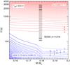 |
Fig. 27 Pulsation periods of our set of low-mass He-core WD models in terms of the stellar mass, for radial (blue dashed lines), non-radial p-modes (blue solid lines) and g modes (red solid lines) at Teff, roughly the effective temperature measured for J111215.82+111745.0. Horizontal black segments (framed in a grey rectangle) represent the periods exhibited by this pulsating star. |
In Fig. 27 we plot the pulsation periods of our set of models in terms of M∗, for radial modes (ℓ = 0) and non-radial p and g modes with ℓ = 1 at roughly the spectroscopic effective temperature derived for J111215.82+111745.0 (Teff = 9590 ± 140 K). The mass assumed for this star, M∗ = (0.179 ± 0.0012) M⊙ is that derived by Althaus et al. (2013) according to the spectroscopic estimation of the surface gravity (log g = 6.36 ± 0.06) as quoted by Hermes et al. (2013a, their Table 4). The periods exhibited by this star (107.5600 s, 134.2750 s, 1792.905 s, 1884.599 s, 2258.528 s, 2539.695 s, 2855.728 s; Hermes et al. 2013b) are indicated by horizontal black segments. Clearly, the long-period pulsations are well accounted for by high radial-order g modes (18 ≲ k ≲ 30). However, at the effective temperature and mass (gravity) of SDSS J111215.82+111745.0 as predicted by spectroscopy, our models are unable to explain the presence of the short periods. They lie in the forbidden region in between g and p modes. An alternative might be to consider modes with higher harmonic degree. In Fig. 28 we show the results for ℓ = 2. Even in this case, the short periods exhibited by SDSS J111215.82+111745.0 are not accounted for by our models, although now they are very close to the lowest-order g-mode periods. We did not perform pulsation computations for higher harmonic degrees, but we expect that the periods at 107.5600 s, 134.2750 s can readily been accounted for by low-order g modes with ℓ = 3. In this case, however, it would be difficult to conceive the detection of ℓ = 3 modes due to geometric cancellation effects (Dziembowski 1977). If we relax the constraint of the stellar mass (gravity), these short periods might be attributed to low-order p modes and/or radial modes, if the stellar mass were somewhat lower (M∗ ~ 0.16 M⊙). Alternatively, they might be associated with low-order g modes if the stellar mass were substantially larger (M∗ ~ 0.43 M⊙). Finally, we might relax the constraint imposed by the effective temperature to determine whether we can accommodate the short periods observed with theoretical periods. The width of the gap between p and g modes decreases slightly for higher effective temperatures (see Fig. 19). However, since the sensitivity of the periods with the effective temperature is by far weaker than with the stellar mass (see Sect. 3.3), the change in the periods (for reasonable variations of Teff) is insufficient for the theoretical periods of low-order (k ~ 1 − 3) g and p modes, and radial modes be similar to the observed ones.
In summary, if the temperature and mass (gravity) of SDSS J111215.82+111745.0 are correct, our models are unable to explain the short periods, and in particular, they cannot be attributed to p modes and/or radial modes.
4.2. SDSS J222859.93+362359.6: an ELM WD or a pre-WD star?
The pulsating ELM WD star SDSS J222859.93+362359.6 is the coolest pulsating WD known so far, with Teff = 7870 ± 120 K. At this low effective temperature, it is remarkably cooler than the other pulsating objects of the class. That this star pulsates at all is somewhat surprising because there are many ELM WDs that do not pulsate in between of this star and SDSS J161431.28+191219.4, the second-coldest pulsating object (Teff = 8800 ± 170 K). Figure 2 reveals the very interesting fact that the star SDSS J222859.93+362359.6 has Teff and log g values that are degenerate with those of more massive pre-WDs that are undergoing a CNO flash episode. This occurs for pre-WD tracks of the sequences with M∗ = 0.3624 M⊙, M∗ = 0.3605 M⊙, M∗ = 0.2707 M⊙, M∗ = 0.2389 M⊙, M∗ = 0.2019 M⊙, and M∗ = 0.1805 M⊙6. This makes it natural to wonder whether the star is a genuine ELM WD star with a stellar mass of M∗ ~ 0.16 M⊙, or is a more massive pre-WD star going through a CNO flash. The hypothesis that this star might be a pre-WD is interesting on its own and deserves to be explored, even taking into account that the evolution of the pre-WDs is much faster than that of the ELM WDs, and therefore there are far fewer opportunities of observing it. To find some clue, we computed the pulsation spectrum of g modes for a template model belonging to the sequence with M∗ = 0.2389 M⊙ when it is looping through one of its CNO flashes and is briefly located at Teff = 7870 K, log g = 6.03. In Fig. 29 we depict the evolutionary track of the 0.2389 M⊙ sequence and the location of this template model on the Teff − log g diagram. We also include in the analysis a template ELM WD model with similar Teff and log g values and M∗ = 0.1554 M⊙ (see left-hand panel of Fig. 29) to compare its pulsation spectrum with that of the 0.2389 M⊙ pre-WD model.
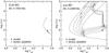 |
Fig. 29 Location of the star SDSS J222859.93+362359.6 (red star symbol) in the log Teff − log g diagram, along with the template ELM WD model on its evolutionary track (left-hand panel) and its twin template pre-WD model with virtually the same Teff/ log g values on its evolutionary track (right-hand panel). |
In Fig. 30 we show the chemical profiles and propagation diagrams of the two template models, including the three frequencies detected in SDSS J222859.93+362359.6. The strongly different internal chemical structure of both models is evident, as is expected because they represent very different evolutionary stages, although they share the same effective temperature and surface gravity. In particular, the pre-WD model (which is going through a CNO flash episode) is characterised by a very thick internal convective zone from r/R∗ ~ 0.3 to r/R∗ ~ 0.9. This convection zone forces most g modes to be strongly confined to the He core (r/R∗ ≲ 0.3), but a few g modes are instead strongly trapped in the H envelope. Note also the very thin outer convection zone, which extends from r/R∗ ~ 0.988 up to r/R∗ = 1. Of course, g modes are evanescent in the convective regions.
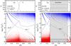 |
Fig. 30 Internal chemical profiles of He and H (upper panels) and the propagation diagrams (lower panels) for the ELM WD template model with M∗ = 0.1554 M⊙ and Teff ≈ 7860 K (left) and the pre-WD template model with M∗ = 0.2389 M⊙ and a similar Teff (right). The grey areas in the 0.2389 M⊙ model indicate a thick inner convective zone at 0.3 ≲ r/R∗ ≲ 0.9 and another, very thin outer convection zone, at 0.988 ≲ r/R∗ ≤ 1. Dashed horizontal lines represent the three frequencies detected in SDSS J222859.93+362359.6. |
The period spacing and kinetic energy of the g modes with ℓ = 1 in terms of periods for both template models are shown in the upper and middle panels of Fig. 31, in which we include, for illustrative purposes, the three periods observed in SDSS J222859.93+362359.6. In addition to a slight difference in the asymptotic period-spacing (ΔΠa = 106.5 s for the ELM WD model, and ΔΠa = 91.85 s for the pre-WD model), very pronnounced minima in ΔΠ appear for the pre-WD model, which are associated with modes with k = 2, k = 17, k = 33, k = 54, and k = 78, which exhibit very low kinetic energies (up to six orders of magnitude lower than the average). These modes are strongly trapped in the outer (radiative) H envelope. They should be easy to excite up to observable amplitudes by virtue of their very low kinetic oscillation energy (low inertia). If this were true, then the spectrum of the pre-WD model should be characterised by a few excited modes with clearly separated periods instead of a continuous spectrum of unstable periods - which should be found, instead, in the 0.1554 M⊙ ELM WD model, by extrapolating to the results of Córsico et al. (2012) for an ELM WD model with M∗ = 0.17 M⊙. If all this were true, the period spectrum of SDSS J222859.93+362359.6, which is itself discrete and composed of only three periods, should be more nearly compatible with the pre-WD model than with the ELM WD model.
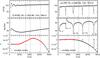 |
Fig. 31 ℓ = 1 period spacing (upper panels), the kinetic oscillation energy (middle panels) and the growth rates (lower panels) in terms of the periods for the template ELM WD model (left) and the template pre-WD model (right). η> 0 implies pulsationally unstable modes. Vertical dashed lines represent the periods observed in SDSS J222859.93+362359.6. |
To test this hypothesis, we computed non-adiabatic pulsations. Specifically, we performed an exploratory stability analysis of the ELM WD sequence with M∗ = 0.1554 M⊙ and the pre-WD sequence with M∗ = 0.2389 M⊙. These computations were carried out with the help of the non-adiabatic version of the LP-PUL pulsation code described in Sect. 2.2. We only computed ℓ = 1g modes with periods in the range of interest and effective temperatures in the range 9000 ≳ Teff ≳ 7400 K, thus embracing the effective temperature of SDSS J222859.93+362359.6 (Teff ~ 7900 K). The output of our code are the normalised non-adiabatic growth rates, η, which are defined as η = −ℑ(σ)/ℜ(σ), where ℜ(σ) and ℑ(σ) are the real and the imaginary part of the complex eigenfrequency σ (see Córsico et al. 2006, for details). Positive values of η mean unstable modes. The growth rates in terms of the pulsation periods are shown in the lower panels of Fig. 31. For the 0.2389 M⊙ pre-WD model, the few modes that are strongly trapped in the H envelope are unstable, as expected. In particular, modes with k = 54 and k = 78 are the only unstable modes for periods Π ≳ 3600 s. The differential work function (see Córsico et al. 2006, for a definition) shows that most of driving for these modes comes from the base of the outer convective zone. Below Π ~ 3600 s we found a continuous band of unstable modes with consecutive radial orders. The differential work functions for these unstable modes indicate that they are excited at the base of the inner convective zone, except for those with k = 2, k = 17, and k = 33, which are trapped in the outer H envelope and are driven at the base of the outer convection zone. On the other hand, the spectrum of unstable modes for the 0.1554 M⊙ ELM WD model consists of a continuous range of periods in the range 800 ≲ Π ≲ 7000 s with consecutive radial orders (8 ≤ k ≤ 64), much in line with the results of Córsico et al. (2012). The k = 1 and k = 2 modes are marginally unstable  . We note that the growth rates η for the unstable modes of the 0.2389 M⊙ model are, on average, more than ten times larger than for the 0.1554 M⊙ model. This indicates that the unstable modes in the pre-WD model are more strongly excited than in the ELM WD model. Finally, in Fig. 32 a more general picture of the situation is shwon. In this plot we depict the unstable periods in terms of the effective temperature for the sequence of pre-WD models with M∗ = 0.1554 M⊙ and for the sequence of ELM WD models with M∗ = 0.2389 M⊙ . We included the three periods detected in SDSS J222859.93+362359.6. The discrete period spectrum of SDSS J222859.93+362359.6 is better represented qualitatively by the period spectrum of unstable modes of the 0.2389 M⊙ pre-WD model sequence than by those of the 0.1554 M⊙ ELM WD sequence.
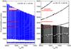 |
Fig. 32 Instability domain on the Teff − Π plane for ℓ = 1g modes for the set of ELM WD models with M∗ = 0.1554 M⊙ (left) and the sequence of pre-WD models with M∗ = 0.2389 M⊙ (right). For the M∗ = 0.1554 M⊙ sequence, the modes with k = 1 and k = 2 are marginally unstable |

In summary, if we accept as valid the possibility that SDSS J222859.93+362359.6 might be a pre-WD star that we are only observing by chance at its brief incursion in the domain of the log Teff − log g diagram where most ELM WDs are found, we would need to explain why we do not observe the continuous period spectrum as predicted by the non-adiabatic computation for the range of periods 200 ≲ Π ≲ 3600 s. Similarly, if we adopt the idea that SDSS J222859.93+362359.6 is a genuine ELM WD star, we need to explain why of the entire continuum spectrum of unstable periods, as predicted by theoretical models, we only observe three isolated periods. All in all, currently we can only state that this star might be a pre-WD instead of an ELM WD, but more observations aimed at detecting additional periods, together with extensive non-adiabatic calculations, are necessary to confirm or discard this statement.
5. Summary and conclusions
We have presented a comprehensive theoretical study of the seismic properties of low-mass, He-core WDs with masses in the range 0.1554 − 0.4389 M⊙. We employed state-of-the-art evolutionary stellar structures representative of these stars, extracted from the sequences of low-mass He-core WDs of Althaus et al. (2013). These models were derived by computing the non-conservative evolution of a binary system consisting of an initially 1 M⊙ ZAMS star and a 1.4 M⊙ neutron star for various initial orbital periods. The evolutionary computations were carried out by accounting for a time-dependent treatment of the gravitational settling and chemical diffusion, as well as of residual nuclear burning. We explored the adiabatic pulsation properties of these models, including the asymptotic predictions, the expected range of periods, period spacings and frequency spacings, the propagation properties and mode trapping of pulsations, as well as the dependence on the effective temperature and stellar mass and the effects of element diffusion. In particular, we strongly emphasised the expected differences in the seismic properties of objects with M∗ ≳ 0.18 M⊙ with CNO flashes during the early-cooling phase, and the ELM WDs (M∗ ≲ 0.18 M⊙) without H flashes.
The pulsation properties of low-mass He-core WDs have been explored in detail recently by Córsico et al. (2012) on the basis of a set of evolutionary models derived by Althaus et al. (2009) considering progenitor stars with supersolar metallicities and single-star evolution. In the present work, we recovered much of the results of Córsico et al. (2012) and extended that study in two ways. First, we explored not only the non-radial g mode pulsation spectrum of low-mass WD models, but also considered non-radial p modes (ℓ = 1,2) and radial (ℓ = 0) pulsation modes. Second, and thanks to the availability of five WD model sequences with progenitors without CNO-flashes (see Table 1), here we were able to explore in detail the pulsation properties of ELM WDs, which are characterised by very thick H envelopes. This is at variance with the work of Córsico et al. (2012), in which only one WD sequence (that with mass M∗ = 0.17 M⊙) belonged to a progenitor star without H flashes. Finally, our study relied on evolutionary models consistent with the expected binary evolution of progenitor stars.
We also discussed how our models match the observed properties of the known five pulsating low-mass WD stars. In particular, we tried to determine whether our models are able to account for the short periods observed in the star SDSS J111215.82+111745.0, and evaluated the possibility that these modes might be p modes and/ radial modes. In addition, we tested the hypothesis that one of these stars, SDSS J222859.93+362359.6, is not a genuine ELM WD, but instead a pre-WD star going through a CNO flash episode.
Although we included some exploratory non-adiabatic pulsation computations, most of our results rely on adiabatic pulsations. We defer a thorough non-adiabatic exploration of our complete set of He-core WD models to a forthcoming paper.
We summarise our findings below.
-
Low-mass WDs have not been clearly classified as ELM WDs in the literature up to now. Here, we proposed to define as ELM WDs the low-mass WDs without CNO flashes in their early-cooling branch. According to this classification, and in the frame of our computations, ELM WDs are the low-mass WDs with masses below ~ 0.18 M⊙. We call stars with M∗ ≳ 0.18 M⊙ LM (low-mass) WDs.
-
The asymptotic period-spacing of g modes in low-mass He-core WDs is larger for lower mass and/or effective temperature. The strong dependence of the period spacing on M∗ might be used to infer the stellar mass of pulsating low-mass WDs, provided that enough consecutive pulsation periods of g modes were detected, although this prospect is complicated by the fact that the period spacing also depends on the thickness of the outer H envelope. In particular, there exist an ambiguity of
for masses near the threshold mass, M∗ ~ 0.18 M⊙. -
The asymptotic frequency-spacing of p modes and radial modes is larger for higher stellar masses and lower effective temperatures.
is insensitive to the thickness of the H envelope. If the detection of this type of modes were confirmed in future observations, the eventual measurement of the mean frequency-spacing for a real star might help to constrain its stellar mass. -
g modes in ELM WDs (M∗ ≲ 0.18 M⊙) mainly probe the core regions and p modes the envelope, which provides the opportunity of constraining both the core and envelope chemical structure of these stars via asteroseismology.
-
For LM WDs, g modes are very sensitive to the He/H compositional gradient and therefore they can be a diagnostic tool for constraining the H-envelope thickness of low-mass WD models with M∗ ≳ 0.18 M⊙.
-
The g-mode periods are longer for smaller mass and lower effective temperature, and in the case of p and radial modes, the periods increase with lower masses and higher effective temperatures. In both cases, the dependence on the effective temperature is much weaker than that on stellar mass.
-
Time-dependent element diffusion strongly affects the g-mode pulsation spectrum of low-mass WDs, in particular ELM WDs. Diffusion processes substantially alter the shape of the He/H chemical interface and in turn the resulting period spectrum. The effects are weaker but still non-negligible for LM WDs. We claim that time-dependent element diffusion must be taken into account in any pulsational analysis of low-mass WD stars.
-
The chemical structure, propagation diagrams, and consequently the pulsation properties of LM WD and ELM WD models with masses near the limit mass (M ~ 0.18 M⊙) are markedly different. These differences are reflected in the period spacing of g modes and the frequency spacing of p modes. For period spacing of g modes, it might be possible to use these differences as a practical tool to distinguish stars with CNO flashes in their early-cooling phase from those without them, provided that enough consecutive low- and intermediate-order g modes with the same harmonic degree were observed in pulsating low-mass WDs. This optimistic view is dampened, however, because the most useful low radial-order g modes are most likely pulsationally stable, as shown from the non-adiabatic analysis of Córsico et al. (2012), and also demonstrated by most of the observed pulsating low-mass WD stars, in which no periods shorter than about 1400 s are seen. Regarding the frequency spacing of p modes, Δνa for the LM WD model is about twice that of the ELM WD model, even though the difference in stellar mass is only ~ 0.004 M⊙. This property might constitute a useful seismological tool if many p mode consecutive periods in pulsating low-mass WDs were detected.
-
Although there are only five pulsating low-mass WDs known at present, and they are not enough in number to trace clear trends of their pulsation spectra, we can note that the observed periods are in general longer for lower gravities and effective temperatures. These trends are in line with theoretical considerations, as discussed by Hermes et al. (2013a).
-
The star SDSS J111215.82+111745.0 exhibits short period pulsations in the range ~ 107 − 140 s. For the temperature and mass (gravity) of this star according to spectroscopy, our models are unable to explain these short periods. In particular, if the temperature and mass (gravity) of the star are correct, the short periods cannot be attributed to p modes and/or radial modes. However, these periods might be caused by low-order p modes and/or radial modes if the stellar mass were lower (M∗ ≈ 0.16 M⊙). Alternatively, they might be low-order g modes if the stellar mass were substantially larger (≈ 0.43 M⊙). Another (unlikely) possibility is that at the spectroscopic mass (gravity) and Teff, the observed periods might be caused by higher-degree (ℓ ≥ 3) low-order g modes.
-
The pulsating ELM WD SDSS J222859.93+362359.6 is the coolest pulsating WD known so far. According to its location in the log Teff − log g plane, this star might be a pre-WD star that is looping through one of its CNO flashes before it enters its final WD cooling track. According to our models, we can neither confirm nor discard this hypothesis at present, although some indications of its discrete period spectrum might promote the idea that the star is a pre-WD star.
Theoretical computations also predict the occurrence of H-shell flashes before the terminal cooling branch is reached even if element diffusion processes are excluded, but in this case, the H envelopes remain thick, with substantial H burning and long WD cooling ages (Driebe et al. 1998; Sarna et al. 2000).
Note that this theoretical mass threshold can vary according to the metallicity of the progenitor stars (Sarna et al. 2000). For instance, Panei et al. (2007), who assumed Z = 0.02 for the progenitor stars, obtained a value ~ 0.17 M⊙ for the mass threshold.
We do not show the results for radial modes because they look very similar to those of p modes.
We recall that the vertical displacements of p modes and radial modes are much smaller than the horizontal displacements of g modes caused by the high gravity, which hinders detecting this type of modes even in low-mass WDs (log g ~ 6).
Note that the same generic trend of periods with Teff is predicted in the frame of the convective driving mechanism, proposed by Brickhill (1990), since in this case the critical timescale is the convective response timescale τC, which itself is some multiple of τth (Montgomery et al. 2008).
A similar situation is found for J111215.82+111745.0 and SDSS J184037.78+642312.3, but in these cases the position of the stars matches only one or two pre-WD tracks.
Acknowledgments
We wish to thank our anonymous referee for the constructive comments and suggestions that greatly improved the original version of the paper. We also warmly thank J. J. Hermes for reading the paper and making enlightening comments and suggestions. Part of this work was supported by AGENCIA through the Programa de Modernización Tecnológica BID 1728/OC-AR, and by the PIP 112-200801-00940 grant from CONICET. This research has made use of NASA Astrophysics Data System.
References
- Althaus, L. G., & Córsico, A. H. 2004, A&A, 417, 1115 [NASA ADS] [CrossRef] [EDP Sciences] [Google Scholar]
- Althaus, L. G., Serenelli, A. M., & Benvenuto, O. G. 2001, MNRAS, 323, 471 [NASA ADS] [CrossRef] [Google Scholar]
- Althaus, L. G., Córsico, A. H., Gautschy, A., et al. 2004, MNRAS, 347, 125 [NASA ADS] [CrossRef] [Google Scholar]
- Althaus, L. G., Serenelli, A. M., Panei, J. A., et al. 2005, A&A, 435, 631 [NASA ADS] [CrossRef] [EDP Sciences] [Google Scholar]
- Althaus, L. G., Panei, J. A., Romero, A. D., et al. 2009, A&A, 502, 207 [NASA ADS] [CrossRef] [EDP Sciences] [Google Scholar]
- Althaus, L. G., Córsico, A. H., Isern, J., & García-Berro, E. 2010, A&ARv, 18, 471 [NASA ADS] [CrossRef] [Google Scholar]
- Althaus, L. G., Miller Bertolami, M. M., & Córsico, A. H. 2013, A&A, 557, A19 [NASA ADS] [CrossRef] [EDP Sciences] [Google Scholar]
- Bassa, C. G. 2006, Ph.D. Thesis, Astronomical Institute, Utrecht University, The Netherlands [Google Scholar]
- Bassa, C. G., van Kerkwijk, M. H., & Kulkarni, S. R. 2003, A&A, 403, 1067 [NASA ADS] [CrossRef] [EDP Sciences] [Google Scholar]
- Beauchamp, A., Wesemael, F., Bergeron, P., et al. 1999, ApJ, 516, 887 [NASA ADS] [CrossRef] [Google Scholar]
- Bradley, P. A., Winget, D. E., & Wood, M. A. 1993, ApJ, 406, 661 [NASA ADS] [CrossRef] [Google Scholar]
- Brassard, P., & Fontaine, G. 1999, in Stellar Structure: Theory and Test of Connective Energy Transport, eds. A. Gimenez, E. F. Guinan, & B. Montesinos, ASP Conf. Ser., 173, 329 [Google Scholar]
- Brassard, P., Fontaine, G., Wesemael, F., & Hansen, C. J. 1992, ApJS, 80, 369 [NASA ADS] [CrossRef] [Google Scholar]
- Brickhill, A. J. 1990, MNRAS, 246, 510 [NASA ADS] [Google Scholar]
- Brown, W. R., Kilic, M., Allen de Prieto, C., & Kenyon, S. J. 2010, ApJ, 723, 1072 [NASA ADS] [CrossRef] [Google Scholar]
- Brown, W. R., Kilic, M., Allen de Prieto, C., & Kenyon, S. J. 2012, ApJ, 744, 142 [NASA ADS] [CrossRef] [Google Scholar]
- Brown, W. R., Kilic, M., Allen de Prieto, C., Gianninas, A., & Kenyon, S. J. 2013, ApJ, 769, 66 [NASA ADS] [CrossRef] [Google Scholar]
- Burgers, J. M. 1969, Flow Equations for Composite Gases (New York: Academic Press) [Google Scholar]
- Cassisi, S., Potekhin, A. Y., Pietrinferni, A., Catelan, M., & Salaris, M. 2007, ApJ, 661, 1094 [NASA ADS] [CrossRef] [Google Scholar]
- Chang, H.-K., Shih, I.-C., Liu, C.-Y., et al. 2013, A&A, 558, A63 [NASA ADS] [CrossRef] [EDP Sciences] [Google Scholar]
- Chen, X., & Han, Z. 2002, MNRAS, 335, 948 [NASA ADS] [CrossRef] [Google Scholar]
- Cohen, J. M., Lapidus, A., & Cameron, A. G. W. 1969, Ap&SS, 5, 113 [NASA ADS] [CrossRef] [Google Scholar]
- Córsico, A. H., & Althaus, L. G. 2006, A&A, 454, 863 [NASA ADS] [CrossRef] [EDP Sciences] [Google Scholar]
- Córsico, A. H., Althaus, L. G., Benvenuto, O. G., & Serenelli, A. M. 2002a, A&A, 387, 531 [NASA ADS] [CrossRef] [EDP Sciences] [Google Scholar]
- Córsico, A. H., Benvenuto, O. G., Althaus, L. G., & Serenelli, A. M. 2002b, MNRAS, 332, 392 [NASA ADS] [CrossRef] [Google Scholar]
- Córsico, A. H., Althaus, L. G., & Miller Bertolami, M. M. 2006, A&A, 458, 259 [NASA ADS] [CrossRef] [EDP Sciences] [Google Scholar]
- Córsico, A. H., Althaus, L. G., Miller Bertolami, M. M., & García-Berro, E. 2009a, J. Phys. Conf. Ser., 172, 012075 [NASA ADS] [CrossRef] [Google Scholar]
- Córsico, A. H., Romero, A. D., Althaus, L. G., & García-Berro, E. 2009b, A&A, 506, 835 [NASA ADS] [CrossRef] [EDP Sciences] [Google Scholar]
- Córsico, A. H., Romero, A. D., Althaus, L. G., & Hermes, J. J. 2012, A&A, 547, A96 [NASA ADS] [CrossRef] [EDP Sciences] [Google Scholar]
- Cox, J. P. 1980, Theory of stellar pulsation (Princeton: Princeton University Press) [Google Scholar]
- Driebe, T., Schoenberner, D., Bloecker, T., & Herwig, F. 1998, A&A, 339, 123 [Google Scholar]
- Dziembowski, W. A. 1971, Acta Astron., 21, 289 [NASA ADS] [Google Scholar]
- Dziembowski, W. 1977, Acta Astron., 27, 203 [NASA ADS] [Google Scholar]
- Ferguson, J. W., Alexander, D. R., Allard, F., et al. 2005, ApJ, 623, 585 [NASA ADS] [CrossRef] [Google Scholar]
- Fontaine, G., & Brassard, P. 2008, PASP, 120, 1043 [NASA ADS] [CrossRef] [Google Scholar]
- García-Berro, E., Torres, S., Althaus, L. G., et al. 2010, Nature, 465, 194 [NASA ADS] [CrossRef] [PubMed] [Google Scholar]
- Grevesse, N., & Sauval, A. J. 1998, Space Sci. Rev., 85, 161 [NASA ADS] [CrossRef] [Google Scholar]
- Haft, M., Raffelt, G., & Weiss, A. 1994, ApJ, 425, 222 [NASA ADS] [CrossRef] [Google Scholar]
- Hermes, J. J., Montgomery, M. H., Winget, D. E., et al. 2012, ApJ, 750, L28 [Google Scholar]
- Hermes, J. J., Montgomery, M. H., Gianninas, A., et al. 2013a, MNRAS, 436, 3573 [NASA ADS] [CrossRef] [Google Scholar]
- Hermes, J. J., Montgomery, M. H., Winget, D. E., et al. 2013b, ApJ, 765, 102 [Google Scholar]
- Iglesias, C. A., & Rogers, F. J. 1996, ApJ, 464, 943 [NASA ADS] [CrossRef] [Google Scholar]
- Itoh, N., Hayashi, H., Nishikawa, A., & Kohyama, Y. 1996, ApJS, 102, 411 [NASA ADS] [CrossRef] [Google Scholar]
- Kawaler, S. D. 1993, ApJ, 404, 294 [NASA ADS] [CrossRef] [Google Scholar]
- Kawaler, S. D., Bond, H. E., Sherbert, L. E., & Watson, T. K. 1994, AJ, 107, 298 [NASA ADS] [CrossRef] [Google Scholar]
- Kepler, S. O., Kleinman, S. J., Nitta, A., et al. 2007, MNRAS, 375, 1315 [NASA ADS] [CrossRef] [Google Scholar]
- Kilic, M., Brown, W. R., Allen de Prieto, C., et al. 2011, ApJ, 727, 3 [NASA ADS] [CrossRef] [Google Scholar]
- Kilic, M., Brown, W. R., Allen de Prieto, C., et al. 2012, ApJ, 751, 141 [NASA ADS] [CrossRef] [Google Scholar]
- Kilkenny, D., Welsh, B. Y., Koen, C., Gulbis, A. A. S., & Kotze, M. M. 2014, MNRAS, 437, 1836 [NASA ADS] [CrossRef] [Google Scholar]
- Kippenhahn, R., Weigert, A., & Weiss, A. 2013, Stellar Structure and Evolution (Berlin, Heidelberg: Springer-Verlag) [Google Scholar]
- Kleinman, S. J., Kepler, S. O., Koester, D., et al. 2013, ApJS, 204, 5 [NASA ADS] [CrossRef] [MathSciNet] [Google Scholar]
- Koester, D., Voss, B., Napiwotzki, R., et al. 2009, A&A, 505, 441 [NASA ADS] [CrossRef] [EDP Sciences] [Google Scholar]
- Landolt, A. U. 1968, ApJ, 153, 151 [NASA ADS] [CrossRef] [Google Scholar]
- Ledoux, P. J., & Sauvenier-Goffin, E. 1950, ApJ, 111, 611 [NASA ADS] [CrossRef] [Google Scholar]
- Magni, G., & Mazzitelli, I. 1979, A&A, 72, 134 [NASA ADS] [Google Scholar]
- Marsh, T. R., Dhillon, V. S., & Duck, S. R. 1995, MNRAS, 275, 828 [NASA ADS] [CrossRef] [Google Scholar]
- Maxted, P. F. L., Anderson, D. R., Burleigh, M. R., et al. 2011, MNRAS, 418, 1156 [NASA ADS] [CrossRef] [Google Scholar]
- Montgomery, M. H., Williams, K. A., Winget, D. E., et al. 2008, ApJ, 678, L51 [NASA ADS] [CrossRef] [Google Scholar]
- Mukadam, A. S., Montgomery, M. H., Winget, D. E., Kepler, S. O., & Clemens, J. C. 2006, ApJ, 640, 956 [NASA ADS] [CrossRef] [Google Scholar]
- Muslimov, A. G., & Sarna, M. J. 1993, MNRAS, 262, 164 [NASA ADS] [CrossRef] [Google Scholar]
- Ostriker, J. P., & Tassoul, J. L. 1969, ApJ, 155, 987 [NASA ADS] [CrossRef] [Google Scholar]
- Panei, J. A., Althaus, L. G., Chen, X., & Han, Z. 2007, MNRAS, 382, 779 [NASA ADS] [CrossRef] [Google Scholar]
- Robinson, E. L. 1984, AJ, 89, 1732 [NASA ADS] [CrossRef] [Google Scholar]
- Rohrmann, R. D., Althaus, L. G., García-Berro, E., Córsico, A. H., & Miller Bertolami, M. M. 2012, A&A, 546, A119 [NASA ADS] [CrossRef] [EDP Sciences] [Google Scholar]
- Romero, A. D., Córsico, A. H., Althaus, L. G., et al. 2012, MNRAS, 420, 1462 [Google Scholar]
- Romero, A. D., Kepler, S. O., Córsico, A. H., Althaus, L. G., & Fraga, L. 2013, ApJ, 779, 58 [NASA ADS] [CrossRef] [Google Scholar]
- Saio, H., Winget, D. E., & Robinson, E. L. 1983, ApJ, 265, 982 [NASA ADS] [CrossRef] [Google Scholar]
- Sarna, M. J., Ergma, E., & Gerškevitš-Antipova, J. 2000, MNRAS, 316, 84 [NASA ADS] [CrossRef] [Google Scholar]
- Siess, L. 2007, A&A, 476, 893 [NASA ADS] [CrossRef] [EDP Sciences] [Google Scholar]
- Silvotti, R., Fontaine, G., Pavlov, M., et al. 2011, A&A, 525, A64 [NASA ADS] [CrossRef] [EDP Sciences] [Google Scholar]
- Silvotti, R., Østensen, R. H., Bloemen, S., et al. 2012, MNRAS, 424, 1752 [NASA ADS] [CrossRef] [Google Scholar]
- Starrfield, S., Cox, A. N., Hodson, S. W., & Clancy, S. P. 1983, ApJ, 269, 645 [NASA ADS] [CrossRef] [Google Scholar]
- Steinfadt, J. D. R., Bildsten, L., & Arras, P. 2010, ApJ, 718, 441 [NASA ADS] [CrossRef] [Google Scholar]
- Steinfadt, J. D. R., Bildsten, L., Kaplan, D. L., et al. 2012, PASP, 124, 1 [NASA ADS] [CrossRef] [Google Scholar]
- Tassoul, M., Fontaine, G., & Winget, D. E. 1990, ApJS, 72, 335 [Google Scholar]
- Tremblay, P.-E., Bergeron, P., & Gianninas, A. 2011, ApJ, 730, 128 [NASA ADS] [CrossRef] [Google Scholar]
- Unno, W., Osaki, Y., Ando, H., Saio, H., & Shibahashi, H. 1989, Nonradial oscillations of stars (University of Tokyo Press) [Google Scholar]
- Van Grootel, V., Dupret, M.-A., Fontaine, G., et al. 2012, A&A, 539, A87 [NASA ADS] [CrossRef] [EDP Sciences] [Google Scholar]
- Van Grootel, V., Fontaine, G., Brassard, P., & Dupret, M.-A. 2013, ApJ, 762, 57 [NASA ADS] [CrossRef] [Google Scholar]
- van Kerkwijk, M. H., Bassa, C. G., Jacoby, B. A., & Jonker, P. G. 2005, in Binary Radio Pulsars, eds. F. A. Rasio, & I. H. Stairs, ASP Conf. Ser., 328, 357 [Google Scholar]
- Vauclair, G. 1971a, in White Dwarfs, ed. W. J. Luyten, IAU Symp., 42, 145 [Google Scholar]
- Vauclair, G. 1971b, Astrophys. Lett., 9, 161 [NASA ADS] [Google Scholar]
- Weiss, A., & Ferguson, J. W. 2009, A&A, 508, 1343 [NASA ADS] [CrossRef] [EDP Sciences] [Google Scholar]
- Winget, D. E., & Kepler, S. O. 2008, ARA&A, 46, 157 [NASA ADS] [CrossRef] [EDP Sciences] [Google Scholar]
All Tables
Selected properties of our He-core WD sequences (final cooling branch) at Teff ≈ 10 000 K: the stellar mass, the mass of H in the outer envelope, the time it takes the star to cool from Teff ≈ 10 000 K to ≈ 8000 K, and the occurrence (or not) of CNO flashes on the early WD cooling branch.
All Figures
|
Fig. 1 Location of the several classes of pulsating WD stars in the log Teff − log g plane, marked with dots of different colours. In parenthesis we include the number of known members of each class. Two post-VLTP (Very Late Thermal Pulse) evolutionary tracks are plotted for reference. We also show the theoretical blue edge of the instability strip for the GW Vir stars, V777 Her stars, the DQV stars (Córsico et al. 2006, 2009a,b, respectively), the ZZ Ceti stars (Fontaine & Brassard 2008), and the pulsating low-mass WDs. For this last class, we show the blue edge according to Hermes et al. (2013a; dotted red line), Córsico et al. (2012; solid red line), and Steinfadt et al. (2010; dashed red line). For reference, we also include two evolutionary tracks of low-mass He-core white dwarfs from Althaus et al. (2013). Small black dots correspond to low-mass WDs that are non-variable or have not been observed yet to assess variability. |
| In the text | |
|
Fig. 2 log Teff − log g diagrams for the He-core WD sequences computed in Althaus et al. (2013). Sequences with masses in the range 0.18 ≲ M∗ ≲ 0.4 undergo CNO flashes during the early-cooling phase, which leads to the complex loops in the diagram. Green squares and magenta triangles correspond to the observed post-RGB low-mass stars from Silvotti et al. (2012) and Brown et al. (2013), and filled blue circles correspond to the five pulsating low-mass WDs detected so far (Hermes et al. 2013a). Numbers in the left upper corner of each panel correspond to the stellar mass at the WD stage. |
| In the text | |
|
Fig. 3 Teff − log g plane showing the low-mass He-core WD evolutionary tracks of Althaus et al. (2013; thin black lines). Sequences with H flashes during the early-cooling phase are depicted with dashed lines, sequences without H flashes are displayed with solid lines. Numbers correspond to the stellar mass of each sequence. The locations of the five known pulsating low-mass WDs (Hermes et al. 2013a) are marked with a small circle (red). Stars not observed to vary are depicted with green triangles. Black circles and squares on the evolutionary tracks of M∗ = 0.1554 M⊙ and M∗ = 0.2389 M⊙ indicate the location of the template models analysed in Sect. 3.2. |
| In the text | |
|
Fig. 4 Dipole (ℓ = 1) asymptotic period spacing of g modes (left panel) and the asymptotic frequency spacing of p modes (right panel) in terms of the effective temperature for all of our low-mass He-core evolutionary sequences. Dashed lines correspond to sequences with CNO flashes during the early-cooling phase, solid lines sequences without H flashes. |
| In the text | |
|
Fig. 5 Internal chemical profiles of He and H (upper panel) and the propagation diagram – the run of the logarithm of the squared critical frequencies (N, Lℓ) – (lower panel) corresponding to the ELM WD template model of M∗ = 0.1554 M⊙ and Teff ≈ 9600 K. Plus symbols (in red) correspond to the spatial location of the nodes of the radial eigenfunction of dipole (ℓ = 1) g modes, x symbols (in blue) represent the location of the nodes of dipole p modes. |
| In the text | |
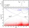 |
Fig. 6 Same as Fig. 5, but for the LM WD template model of M∗ = 0.2389 M⊙. |
| In the text | |
|
Fig. 7 Run of the density of kinetic energy dEekin/dr (normalised to 1) for radial modes (dashed blue) and dipole g (red) and p modes (solid blue curves) with k = 1 (upper panel), k = 10 (middle panel), and k = 60 (lower panel), corresponding to the ELM template model with M∗ = 0.1554 M⊙. The vertical dashed line marks the location of the He/H chemical transition region. |
| In the text | |
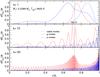 |
Fig. 8 Same as Fig. 7, but for the LM WD template model with M∗ = 0.2389 M⊙. |
| In the text | |
|
Fig. 9 ℓ = 1 forward period-spacing of g modes versus periods (upper left-hand panel), and the forward frequency-spacing of radial modes (hollow small circles) and p modes (filled small circles) versus frequencies (upper right-hand panel) and the associated oscillation kinetic energy distributions (lower panels) for the ELM WD template model with M∗ = 0.1554 M⊙ and Teff ~ 9600 K. The red horizontal lines in the upper panels correspond to the asymptotic period-spacing (left), computed with Eq. (7), and the asymptotic frequency-spacing (right), computed with Eq. (13). |
| In the text | |
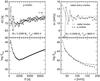 |
Fig. 10 Same as Fig. 9, but for the LM WD template model with M∗ = 0.2389 M⊙ and Teff ~ 9600 K. |
| In the text | |
|
Fig. 11 Chemical profiles of He and H (upper panel) and the propagation diagram (lower panel) for the ELM WD template model of M∗ = 0.1554 M⊙ and Teff ≈ 7800 K. |
| In the text | |
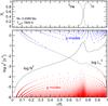 |
Fig. 12 Same as Fig. 11, but for the LM WD template model with M∗ = 0.2389 M⊙. |
| In the text | |
|
Fig. 13 Run of the density of kinetic energy dEekin/dr (normalised to 1) for dipole g (red) and p modes (solid blue curves) with k = 1 (upper panel), k = 10 (middle panel), and k = 60 (lower panel), for the ELM template model with M∗ = 0.1554 M⊙ and Teff ≈ 7800 K (analysed in Fig.11). |
| In the text | |
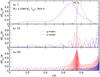 |
Fig. 14 Same as Fig. 13, but for the LM WD template model with M∗ = 0.2389 M⊙ analysed in Fig. 12. |
| In the text | |
|
Fig. 15 ℓ = 1 forward period-spacing of g modes versus periods (upper left-hand panel), and the forward frequency-spacing of radial modes (hollow small circles) and p modes (filled small circles) versus frequencies (upper right-hand panel) and the corresponding kinetic energy distributions (lower panels) for the ELM WD template model with M∗ = 0.1554 M⊙ and Teff ~ 7800 K. |
| In the text | |
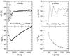 |
Fig. 16 Same as Fig.15, but for the LM WD template model with M∗ = 0.2389 M⊙. |
| In the text | |
|
Fig. 17 Pulsation periods of ℓ = 1g- and p modes and also radial modes (ℓ = 0) in terms of the stellar mass for Teff = 9500 K. Periods increase with decreasing M∗. |
| In the text | |
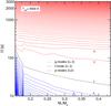 |
Fig. 18 Same as Fig. 17, but for pulsation periods of ℓ = 2g, f, and p modes. |
| In the text | |
|
Fig. 19 Pulsation periods of ℓ = 1g modes and p modes/radial modes in terms of the effective temperature for M∗ = 0.1917 M⊙. g-mode periods increase with decreasing Teff; the opposite holds for p modes and radial modes. |
| In the text | |
|
Fig. 20 Internal chemical profile of H (upper panel), the Ledoux term B entering in the computation of the Brunt-Väisälä frequency (see Eq. (11)) (middle panel), and the logarithm of the squared Brunt-Väisälä frequency (lower panel), for an ELM WD model with M∗ = 0.1554 M⊙ at different effective temperatures, as indicated. |
| In the text | |
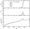 |
Fig. 21 Same as Fig. 20, but for an LM WD model with M∗ = 0.2389 M⊙. |
| In the text | |
|
Fig. 22 Chemical profiles of He and H (upper panel), the propagation diagram (centre panel), and the kinetic energy density for dipole g (red) and p modes (solid blue curves) with k = 1,10, and 20 (lower panels), for an ELM WD model with M∗ = 0.1762 M⊙ and Teff ≈ 10 000 K. |
| In the text | |
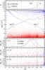 |
Fig. 23 Same as Fig. 22, but for an LM WD model with M∗ = 0.1806 M⊙. |
| In the text | |
|
Fig. 24 Upper panels: ℓ = 1 forward period-spacing of g modes vs. periods. Lower panels: forward frequency-spacing of p modes vs. frequency. Left-hand panels: ELM WD model with M∗ = 0.1762 M⊙. Right-hand panels: LM WD model with M∗ = 0.1805 M⊙, both at Teff ~ 10 000 K. Red dashed lines correspond to the asymptotic predictions. |
| In the text | |
|
Fig. 25 Pulsation periods of the five known pulsating low-mass WD stars in terms of the effective temperature, according to Table 4 of Hermes et al. (2013a). |
| In the text | |
|
Fig. 26 Pulsation periods of the five known pulsating low-mass WD stars in terms of the surface gravity, according to Table 4 of Hermes et al. (2013a). |
| In the text | |
|
Fig. 27 Pulsation periods of our set of low-mass He-core WD models in terms of the stellar mass, for radial (blue dashed lines), non-radial p-modes (blue solid lines) and g modes (red solid lines) at Teff, roughly the effective temperature measured for J111215.82+111745.0. Horizontal black segments (framed in a grey rectangle) represent the periods exhibited by this pulsating star. |
| In the text | |
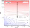 |
Fig. 28 Same as Fig. 27, but for non-radial ℓ = 2p, f, and g modes. |
| In the text | |
|
Fig. 29 Location of the star SDSS J222859.93+362359.6 (red star symbol) in the log Teff − log g diagram, along with the template ELM WD model on its evolutionary track (left-hand panel) and its twin template pre-WD model with virtually the same Teff/ log g values on its evolutionary track (right-hand panel). |
| In the text | |
|
Fig. 30 Internal chemical profiles of He and H (upper panels) and the propagation diagrams (lower panels) for the ELM WD template model with M∗ = 0.1554 M⊙ and Teff ≈ 7860 K (left) and the pre-WD template model with M∗ = 0.2389 M⊙ and a similar Teff (right). The grey areas in the 0.2389 M⊙ model indicate a thick inner convective zone at 0.3 ≲ r/R∗ ≲ 0.9 and another, very thin outer convection zone, at 0.988 ≲ r/R∗ ≤ 1. Dashed horizontal lines represent the three frequencies detected in SDSS J222859.93+362359.6. |
| In the text | |
|
Fig. 31 ℓ = 1 period spacing (upper panels), the kinetic oscillation energy (middle panels) and the growth rates (lower panels) in terms of the periods for the template ELM WD model (left) and the template pre-WD model (right). η> 0 implies pulsationally unstable modes. Vertical dashed lines represent the periods observed in SDSS J222859.93+362359.6. |
| In the text | |
|
Fig. 32 Instability domain on the Teff − Π plane for ℓ = 1g modes for the set of ELM WD models with M∗ = 0.1554 M⊙ (left) and the sequence of pre-WD models with M∗ = 0.2389 M⊙ (right). For the M∗ = 0.1554 M⊙ sequence, the modes with k = 1 and k = 2 are marginally unstable |
| In the text | |
Current usage metrics show cumulative count of Article Views (full-text article views including HTML views, PDF and ePub downloads, according to the available data) and Abstracts Views on Vision4Press platform.
Data correspond to usage on the plateform after 2015. The current usage metrics is available 48-96 hours after online publication and is updated daily on week days.
Initial download of the metrics may take a while.