| Issue |
A&A
Volume 569, September 2014
|
|
|---|---|---|
| Article Number | A44 | |
| Number of page(s) | 10 | |
| Section | Astrophysical processes | |
| DOI | https://doi.org/10.1051/0004-6361/201423819 | |
| Published online | 16 September 2014 | |
Self-consistent stationary MHD shear flows in the solar atmosphere as electric field generators
1
Astronomical Institute,
AV ČR, Fričova 298,
25165
Ondřejov,
Czech Republic
e-mail:
This email address is being protected from spambots. You need JavaScript enabled to view it.
2
Max-Planck Institut für Sonnensystemforschung,
Justus-von-Liebig-Weg
3, 37077
Göttingen,
Germany
Received:
16
March
2014
Accepted:
2
July
2014
Abstract
Context. Magnetic fields and flows in coronal structures, for example, in gradual phases in flares, can be described by 2D and 3D magnetohydrostatic (MHS) and steady magnetohydrodynamic (MHD) equilibria.
Aims. Within a physically simplified, but exact mathematical model, we study the electric currents and corresponding electric fields generated by shear flows.
Methods. Starting from exact and analytically calculated magnetic potential fields, we solved the nonlinear MHD equations self-consistently. By applying a magnetic shear flow and assuming a nonideal MHD environment, we calculated an electric field via Faraday’s law. The formal solution for the electromagnetic field allowed us to compute an expression of an effective resistivity similar to the collisionless Speiser resistivity.
Results. We find that the electric field can be highly spatially structured, or in other words, filamented. The electric field component parallel to the magnetic field is the dominant component and is high where the resistivity has a maximum. The electric field is a potential field, therefore, the highest energy gain of the particles can be directly derived from the corresponding voltage. In our example of a coronal post-flare scenario we obtain electron energies of tens of keV, which are on the same order of magnitude as found observationally. This energy serves as a source for heating and acceleration of particles.
Key words: magnetohydrodynamics (MHD) / Sun: flares / Sun: corona / methods: analytical
© ESO, 2014
1. Introduction
Dissipation or acceleration processes of energized particles occur in a variety of astrophysical plasma environments. For example, acceleration of charged particles is observed in the heliosphere, where anomalous cosmic rays are accelerated to high energies (see, e.g., Drake et al. 2010; Giacalone et al. 2012), in the Earth magnetotail and aurorae (e.g., Birn et al. 2012), and in solar flares (see, e.g., Miller 1998; Aschwanden 2002) and nanoflares (e.g., Bingert & Peter 2011), where electrons and ions are heated and accelerated. These processes are typically connected with strong electric currents and electric fields. A reasonable approach for computing these electric fields and currents is provided by the theory of magnetohydrodynamics (MHD). But while MHD simulations compute solutions only on pre-defined grid points, meaning that values of the electromagnetic field have to be interpolated, analytical MHD configurations have the advantage of providing exact knowledge of the electromagnetic field at every point in space. Therefore, exact analytical MHD configurations are ideal as background fields in test particle simulations.
To trigger dissipation, for instance, in the form of Ohmic heating, or acceleration, a parallel component of the electric field with respect to the magnetic field must exist. Such electric field components parallel to the magnetic field can be obtained from nonideal MHD.
The heating of the solar plasma and the acceleration of charged particles during solar flare events is a long-standing problem. Three different main mechansisms have been described (for a detailed review see Aschwanden 2002): (i) DC-electric field acceleration, which is typically connected to magnetic collapse processes (magnetic reconnection such as collapsing magnetic loops and the magnetic mirror effect, Karlický & Bárta 2007) or via the Betatron mechanism (Karlický & Kosugi 2004), (ii) stochastic acceleration caused by wave-particle interaction, so-called weak turbulence (e.g., Miller 1998; Lazarian & Vishniac 1999), and (iii) shock acceleration.
The scenario of DC-electric field acceleration is very promising, in particular for the aftermath of a solar flare event, where magnetic reconnection had taken place and a plasmoid was ejected. In such a reconnection region, strong electric fields are generated, which can directly accelerate charged particles. These particles are traced by their X-ray emission. However, after the new equilibrium state is reached, the main magnetic field component of such a post-flare configuration is the poloidal magnetic field, which can typically be described by a potential field. This can be justified by the fact that after the impulsive phase the main component of the field should be relaxed. However, the “bursty” reconnection event itself is not sufficient to explain the observed slow decay in intensity of the X-ray observations taken immediately after the impulsive phase (see, e.g., Kane 1974). This behavior of the emission speaks in favor of a continous (although reduced) acceleration on much longer timescales. If the relaxed configuration would consist of a pure potential field, this would imply that no further dissipation can take place and particle acceleration has stopped, in contrast to what is observed. Hence, particles must also be accelerated in the (almost) relaxed magnetic field. Therefore, a current-producing shear component must exist, which provides a reasonably strong electric field component that is necessary to accelerate charged particles along the field lines. Such shear fields have been observed (see, e.g., Wang 1992).
In this paper we investigate the influence of shear flows on the generation of electric fields with component parallel to the magnetic field in a typical post-flare configuration. In numerical test-particle approaches, as has been critically commented on by, e.g., Brown et al. (2009) and Zharkova et al. (2011), the particles are passive, which means that the feedback of the moving charges is not taken into account. This could be done numerically by considering a kinetic approach. However, because in kinetic models spatial and time scales have to be resolved, which requires quite different scales (Debye length and gyro-frequency), this treatment is numerically expensive. In contrast, our exact analytical nonideal MHD model allows us to precisely compute the field everywhere, not only on a predefined grid. In addition, our treatment of the accelerated bulk particles automatically includes the nonlinear feedback between the plasma and the electromagnetic field, which emphasizes the advantage of exact analytical models.
2. Theoretical approach
2.1. Derivation of the MHD model
In typical simulation scenarios a shear is applied to the footpoints of solar arcade structures (see, e.g., Leake et al. 2013, and references therein). Then the system relaxes into a new state. However, this new state is not necessarily an exact equilibrium state. Because we aim at an exact steady-state for our model considerations, we have to follow a strategy that allows us to compute the exact final state into which the system relaxes. This is offered by the transformation theory, which was developed by Gebhardt & Kiessling (1992). The transformation method allows us to calculate steady ideal MHD equilibria with field-aligned incompressible flow from known MHS equilibria (see, e.g., Petrie & Neukirch 1999; Nickeler et al. 2006, 2013; Nickeler & Wiegelmann 2010, 2012), and it is applied here to obtain a stationary equilibrium, consisting of a poloidal field and a shear component in z-direction, from an originally pure potential field. Our chosen coordinate system is such that the y-axis is perpendicular to the solar surface (pointing upward), and the x-axis is tangential. The z-axis is tangential as well and points out of the (poloidal) plane in all our graphics.
We start from the set of stationary MHD equations for field-aligned, incompressible
flows, given by 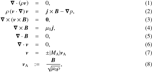 where
ρ is the
mass density, v is the plasma velocity,
B is the magnetic flux density,
j is the current density,
p is the
plasma pressure, MA is the Alfvén Mach number,
vA is the Alfvén velocity,
and μ0 is the magnetic permeability of the
vacuum. The gravitational force in the considered domains of our model is at least a
factor 100 lower than the Lorentz-force, so that the influence of gravity in our approach
can be neglected.
where
ρ is the
mass density, v is the plasma velocity,
B is the magnetic flux density,
j is the current density,
p is the
plasma pressure, MA is the Alfvén Mach number,
vA is the Alfvén velocity,
and μ0 is the magnetic permeability of the
vacuum. The gravitational force in the considered domains of our model is at least a
factor 100 lower than the Lorentz-force, so that the influence of gravity in our approach
can be neglected.
In the current work we focus on solar magnetic arcade structures, implying translational
invariance. This justifies restricting our investigations to 2.5D magnetic field
configurations, that is, ∂/∂z = 0 for all
our variables, although the transformation used could also be applied to full 3D
scenarios. In addition to the translational invariance, we assume that there is no
electric current component in the invariant (here z) direction, that is,
jz = 0. As
jz = 0, we have to
solve the Laplace equation ΔA
= 0 for the flux function A or Δφm = 0 for the complex
conjugated vector potential φm. This is commonly
achieved by complex analysis. Hence we define by φm and A the complex conjugated
potentials of the complex magnetic vector potential
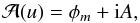 (9)with u = x +
iy. These potentials fulfill the Cauchy-Riemann
equations ∇φm =
∇A ×
ez and,
therefore, obey the condition ∇φm·∇A
= 0. To determine the magnetic potential φm and the flux function
A, the
Laplace equation is solved by expressing
(9)with u = x +
iy. These potentials fulfill the Cauchy-Riemann
equations ∇φm =
∇A ×
ez and,
therefore, obey the condition ∇φm·∇A
= 0. To determine the magnetic potential φm and the flux function
A, the
Laplace equation is solved by expressing  with Laurent series, applying asymptotical boundary conditions.
With the magnetic potentials, we can use the potential field ∇φm to
define the static poloidal magnetic field Bps in the form
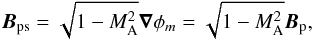 (10)where ∇φm
= Bp is the stationary
poloidal magnetic field and MA is the constant Alfvén Mach number.
The requirement of MA = const follows from the fact that on
the one hand, Bps is a potential field,
and on the other hand, no current is generated in z-direction by the
transformation. For simplicity, to have the representation of the stationary magnetic
field in the usual form via ∇φm, we
introduced the factor
(10)where ∇φm
= Bp is the stationary
poloidal magnetic field and MA is the constant Alfvén Mach number.
The requirement of MA = const follows from the fact that on
the one hand, Bps is a potential field,
and on the other hand, no current is generated in z-direction by the
transformation. For simplicity, to have the representation of the stationary magnetic
field in the usual form via ∇φm, we
introduced the factor  into the static poloidal magnetic field, which vanishes identically after the
transformation has been applied. For the current investigation, we considered only
sub-Alfvénic flows, which means that
into the static poloidal magnetic field, which vanishes identically after the
transformation has been applied. For the current investigation, we considered only
sub-Alfvénic flows, which means that  . The
initial potential magnetic field Bps together with the
static plasma pressure ps0 = const define the starting MHS
equilibrium.
. The
initial potential magnetic field Bps together with the
static plasma pressure ps0 = const define the starting MHS
equilibrium.
To compute the stationary MHD equilibrium, we applied a 2.5D shear flow v and
simultaneously performed the transformation, so that we obtained a self-consistent 2.5D
MHD flow. While the x and y components of the shear flow are functions of the
poloidal magnetic field, the z component produces a nonconstant magnetic shear
Bz =
Bz(A)
in z-direction, given by 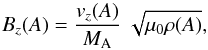 (11)where ρ(A) is
the plasma density. As was shown by Nickeler et al.
(2006), the density is an explicit function of A. To fulfill the
requirement of a field-aligned flow, the shear flow has to have the following structure
(11)where ρ(A) is
the plasma density. As was shown by Nickeler et al.
(2006), the density is an explicit function of A. To fulfill the
requirement of a field-aligned flow, the shear flow has to have the following structure
 (12)From the
transformation and the application of the shear the stationary magnetic field has the form
(12)From the
transformation and the application of the shear the stationary magnetic field has the form
 (13)and the electric
current is given by Ampère’s law,
(13)and the electric
current is given by Ampère’s law,  The
prime denotes the derivative with respect to A, that is,
The
prime denotes the derivative with respect to A, that is,  . The thermal pressure of
the sheared equilibrium is
. The thermal pressure of
the sheared equilibrium is  (16)The parameter
ps in Eq. (16) is the static pressure of an equilibrium state like ours plus a
shear component. This means that we define the total static pressure as
(16)The parameter
ps in Eq. (16) is the static pressure of an equilibrium state like ours plus a
shear component. This means that we define the total static pressure as
 , with ps0 as the
static pressure of the pure poloidal field. The thermal pressure (Eq. (16)) together with the flow (Eq. (12)) and the magnetic field (Eq. (13)) self-consistently fulfill the
incompressible ideal steady-state MHD equations with field-aligned flows.
, with ps0 as the
static pressure of the pure poloidal field. The thermal pressure (Eq. (16)) together with the flow (Eq. (12)) and the magnetic field (Eq. (13)) self-consistently fulfill the
incompressible ideal steady-state MHD equations with field-aligned flows.
In ideal MHD, Ohm’s law is given by
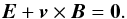 (17)The use of
field-aligned flows, which implies that v × B =
0, has a severe consequence, because such an
electro-magnetic field configuration in ideal MHD cannot accelerate injected charged
particles because the electric field is zero. To guarantee particle acceleration, we must
rely on resistive MHD, using resistive Ohm’s law given by
(17)The use of
field-aligned flows, which implies that v × B =
0, has a severe consequence, because such an
electro-magnetic field configuration in ideal MHD cannot accelerate injected charged
particles because the electric field is zero. To guarantee particle acceleration, we must
rely on resistive MHD, using resistive Ohm’s law given by
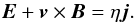 (18)In this scenario an
electric field also exists for field-aligned flows, but only for ηj ≠
0 and hence in particular for η ≠ 0.
(18)In this scenario an
electric field also exists for field-aligned flows, but only for ηj ≠
0 and hence in particular for η ≠ 0.
To enable quasi-steady and sustainable electric fields with field-aligned flows, it is necessary to simultaneously solve the resistive Ohm’s law and the momentum equation. This was first investigated by Grad & Hogan (1970) and subsequently by Throumoulopoulos (1998) and Throumoulopoulos & Tasso (2000) for the case of axisymmetric fields. These authors found several classes of analytical equilibria with physically plausible σ = 1/η profiles, stating clearly that in general, fields with constant resistivity do not exist by proving that only the assumption of a spatially varying σ makes the equilibrium problem well posed. In addition, they found that according to Ohm’s law η is determining the MHD solutions, but η is also determined by constraints concerning the geometry of flow and field. Therefore, we applied a similar concept of a nonconstant resistivity for our translational invariant model.
The steady-state Maxwell equation ∇ × E = −
∂B/∂t
= 0 implies the existence of an electric potential
φe so that − ∇φe =
E =
ηj. Because the
Cauchy-Rieman differential equations imply that ∇φm·∇A
= 0, we can choose φm and A as orthogonal
coordinates. This allows us to consider the electric potential φe as a function
of the magnetic potential field φm and the flux
function A.
With the current, given by Eq. (14), we can
re-write the identity ηj = −
∇φe in the form
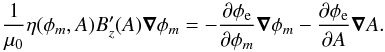 (19)A comparison of the
coefficients delivers that ∂φe/∂A
= 0, which means that the electric potential φe is an
explicit function of φm only, and
therefore
(19)A comparison of the
coefficients delivers that ∂φe/∂A
= 0, which means that the electric potential φe is an
explicit function of φm only, and
therefore 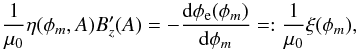 (20)where
 , which has the SI unit Ohm,
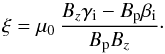
can be regarded as the resistance of the plasma. Furthermore, we find from Eq. (20) for the electric potential φe
, which has the SI unit Ohm,
can be regarded as the resistance of the plasma. Furthermore, we find from Eq. (20) for the electric potential φe (21)Consequently,
equipotential surfaces of the scalar potential φm of the poloidal
magnetic field are also equipotential surfaces of the electric potential, φe =
φe(φm).
(21)Consequently,
equipotential surfaces of the scalar potential φm of the poloidal
magnetic field are also equipotential surfaces of the electric potential, φe =
φe(φm).
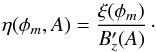
Considering the different representations, the electric field can be written in various
equivalent forms:  The
existence of an electric field component aligned with the magnetic field provides an
energy gain and hence an acceleration of charged particles along the field lines. The
computation of the total electric field (and hence the parallel component) explicitly
depends on the resistivity η, but implicitly on the resistance ξ. In the scenario of a
post-flare configuration described above, which neglects currents in the invariant
direction and an electric field component produced by the flow, we found that the
resistivity is given by (see Eq. (20))
The
existence of an electric field component aligned with the magnetic field provides an
energy gain and hence an acceleration of charged particles along the field lines. The
computation of the total electric field (and hence the parallel component) explicitly
depends on the resistivity η, but implicitly on the resistance ξ. In the scenario of a
post-flare configuration described above, which neglects currents in the invariant
direction and an electric field component produced by the flow, we found that the
resistivity is given by (see Eq. (20))
 (24)Although the resistivity
is an explicit function of the two complex conjugated potentials φm and A, it is very special in
the sense that the two coordinates appear separately in the two functions ξ and
(24)Although the resistivity
is an explicit function of the two complex conjugated potentials φm and A, it is very special in
the sense that the two coordinates appear separately in the two functions ξ and
 that
determine η.
that
determine η.
The resistance, ξ, and the derivative of the magnetic shear,
, can
basically be chosen independently. To investigate the properties of this resistivity, we
discuss various options for functions ξ and in the
following. The case of a constant magnetic shear component can directly be excluded
because this would imply that  and hence the configuration
would contain no currents and the resistivity would be undefined. For a nonconstant
magnetic shear component we are left with four different possibilities: (i)
and hence the configuration
would contain no currents and the resistivity would be undefined. For a nonconstant
magnetic shear component we are left with four different possibilities: (i)
 is constant and ξ is constant; (ii)
is constant and ξ is not constant; (iii)
is nonconstant but
ξ is
constant; and (iv) and ξ are both nonconstant.
is constant and ξ is constant; (ii)
is constant and ξ is not constant; (iii)
is nonconstant but
ξ is
constant; and (iv) and ξ are both nonconstant.
If ξ and
were both constant, the
resistivity would be constant as well, meaning that the electric field only depends on the
poloidal magnetic field (see Eq. (22)).
Hence, a strong electric field would only occur in regions of high magnetic field
strength, for example, in regions of high current density (see Eq. (14)). Such regions of high current density
occur close to the poles of multipolar regions, for instance. If
is constant and ξ is not constant,
η only
depends on φm and only varies in
direction along the magnetic field lines. If  constant,
η will
decrease with increasing , but the choice of the function
ξ enables
us to receive a high resistivity at specific locations. Hence choosing a constant
ξ is
unsuitable because it prevents a change and localization of the electric field along the
magnetic field lines and therefore an effective concentration of the particle acceleration
engine.
constant,
η will
decrease with increasing , but the choice of the function
ξ enables
us to receive a high resistivity at specific locations. Hence choosing a constant
ξ is
unsuitable because it prevents a change and localization of the electric field along the
magnetic field lines and therefore an effective concentration of the particle acceleration
engine.
The search for appropriate expressions for the resistivity is additionally hampered by the fact that in cases of nonconstant ξ one has to find a physical explanation for ξ, which is not obvious a priori. Evidently, ξ represents a characteristic electric resistance, which depends on the distance along the magnetic field lines.
A high resistivity alone is not sufficient for the occurrence of strong (parallel) electric fields. Instead, appropriate choices for the spatial distributions of both the poloidal magnetic field and the function ξ are required. The regions where the conditions for the appearance of strong electric fields are met are, therefore, not necessarily identical to those where the effective resistivity η is particularly high. Nevertheless, we need a physical explanation for the resistivity and a reasonable physical correlation between resistivity and the function ξ. The Spitzer resistivity is not valid for solar corona or solar flare scenarios because the density is too low, which prevents efficient collisions between particles. On the other hand, the turbulent collisionless resistivity (anomalous resistivity due to wave-particle interactions), which occurs during eruptive procsses such as impulsive phases of flares, is usually not stationary. Therefore, the most appropriate approach for our investigations is to find a stationary resistivity that takes noncollisional effects into account.
2.2. Geometrical approach for the noncollisional inertia-induced resistivity: Speiser-like approach
The resistivity in our model depends on the resistance ξ, which was defined in Eq.
(20) as a function of the vector
potential φm. The resistance
ξ(φm)
and the resistivity  define formally exact solutions
for the resistivity and the electric field in the specific geometry of a given magnetic
field, but for estimating the “amplitude”, that is, the absolute value of ξ and thus η, a quantitative approach
is required. To estimate a noncollisional but steady-state η it is hence essential to
derive a parameterization for the resistance. For this, we make a short excursion into the
two-fluid approach. Here, the resistance ξ can be represented by utilizing the ideas of the
so-called Speiser conductivity (Speiser
1970), which is based on the inertia of the injected and accelerated charged
particles. This means that we are using stationary movements of particles to derive the
relation between the total electric fields (see Eqs. (25) and (26) below)
and ξ. This
procedure can be justified by the suggestion of Speiser (see, e.g., Speiser 1968, 1970; Dungey & Speiser 1969), who stated
that the effect of particle inertia can be more important in determining the relation
between E and j in a
collisionless plasma than wave-particle interactions.
define formally exact solutions
for the resistivity and the electric field in the specific geometry of a given magnetic
field, but for estimating the “amplitude”, that is, the absolute value of ξ and thus η, a quantitative approach
is required. To estimate a noncollisional but steady-state η it is hence essential to
derive a parameterization for the resistance. For this, we make a short excursion into the
two-fluid approach. Here, the resistance ξ can be represented by utilizing the ideas of the
so-called Speiser conductivity (Speiser
1970), which is based on the inertia of the injected and accelerated charged
particles. This means that we are using stationary movements of particles to derive the
relation between the total electric fields (see Eqs. (25) and (26) below)
and ξ. This
procedure can be justified by the suggestion of Speiser (see, e.g., Speiser 1968, 1970; Dungey & Speiser 1969), who stated
that the effect of particle inertia can be more important in determining the relation
between E and j in a
collisionless plasma than wave-particle interactions.
Differently from the situation in the Speiser models, the geometry used in our models is more complicated: our models are 2.5D while the Speiser models were 1.5D (see e.g. Lyons & Speiser 1985). In addition, our current sheet is not given by the Maxwellian jump condition with respect to the main componentBp of the magnetic field, but by the shear componentBz.
In our model we assume that a steady-state flow of coronal material can develop in which the plasma streams along the field lines that have been sheared in z-direction. However, within this ordered plasma stream, a drift between the different species of charged particles (electrons and protons or ions) can be expected. The drift inside the global plasma flow initiates a current, which is, via Ampère’s law, related to a magnetic shear component. Hence, no turbulent approach is needed to obtain an electric field. Instead, it results naturally from the inertial forces.
The inertial forces acting on the charged particles generated by the electric and
magnetic fields can be written as 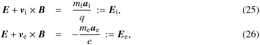 where
vi and ve
are the velocity fields of the charged particles (ions i and electrons e), mi and
me are their masses, ai
and ae are the accelerations
acting on the bulk of particles, and q and e are their charges. The coupling between the
Maxwell equation (Ampère’s law) and the fluid equations is realized via Eqs. (30), (31) and (33) below. Here, we
explicitly considered only the electric force and the Lorentz force, while all other
collective forces (like ∇Pe, the Hall term, etc.)
are included in the total electric field for each species (ions Ei
and electrons Ee). The forces
Fi,e =
mi,eai,e
are proportional to the total electric fields Ei,e (= the electric
field that particles encounter in the comoving frame). If we solve for the velocity fields
vi,e,
the general solution of the force Eqs. (25) and (26) is
where
vi and ve
are the velocity fields of the charged particles (ions i and electrons e), mi and
me are their masses, ai
and ae are the accelerations
acting on the bulk of particles, and q and e are their charges. The coupling between the
Maxwell equation (Ampère’s law) and the fluid equations is realized via Eqs. (30), (31) and (33) below. Here, we
explicitly considered only the electric force and the Lorentz force, while all other
collective forces (like ∇Pe, the Hall term, etc.)
are included in the total electric field for each species (ions Ei
and electrons Ee). The forces
Fi,e =
mi,eai,e
are proportional to the total electric fields Ei,e (= the electric
field that particles encounter in the comoving frame). If we solve for the velocity fields
vi,e,
the general solution of the force Eqs. (25) and (26) is 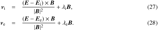 The
free parameters λi,e of the general
solution correspond to the Alfvén Mach number of the flows of the particular particle
species:
The
free parameters λi,e of the general
solution correspond to the Alfvén Mach number of the flows of the particular particle
species:  (29)The
electric current is typically given by the drift between the different charges
(29)The
electric current is typically given by the drift between the different charges
 (30)On the other hand, in
the MHD picture the current is generated by the magnetic shear (see Eq. (14))
(30)On the other hand, in
the MHD picture the current is generated by the magnetic shear (see Eq. (14))  (31)As both
expressions have to be equal, we can compare the coefficients. For this, we introduce a
new orthogonal coordinate system defined by the basis
(31)As both
expressions have to be equal, we can compare the coefficients. For this, we introduce a
new orthogonal coordinate system defined by the basis
 .
The superscript 0 denotes that
the vectors are normalized. Then we can express the physical parameters in this new
coordinate system: The poloidal magnetic field can be written as Bp =
Bp(∇φm)0,
and the total electric fields that are needed to compute the particle velocities become
.
The superscript 0 denotes that
the vectors are normalized. Then we can express the physical parameters in this new
coordinate system: The poloidal magnetic field can be written as Bp =
Bp(∇φm)0,
and the total electric fields that are needed to compute the particle velocities become
 (32)where α,β, and γ are the coordinates of
the corresponding basis. The relation for the current density can thus be written in the
form
(32)where α,β, and γ are the coordinates of
the corresponding basis. The relation for the current density can thus be written in the
form 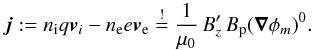 (33)The expressions
for the velocities, Eqs. (27) and (28), and a comparison of coefficients with
respect to the orthogonal unit vectors result in three conditions for the electric field
components of the two species:
(33)The expressions
for the velocities, Eqs. (27) and (28), and a comparison of coefficients with
respect to the orthogonal unit vectors result in three conditions for the electric field
components of the two species: 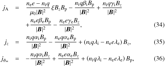 with
the projection in the direction of the three coordinates of the three basis vectors,
namely
with
the projection in the direction of the three coordinates of the three basis vectors,
namely 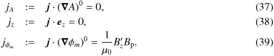 Because
only jA contains the
resistance ξ,
we concentrate on this component to receive a relation coupling the physical parameters
Bp, Bz, ξ, and η. This coupling can only
be calculated if nee −
niq in the nominator of
the first term on the right-hand side of Eq. (34) does not vanish. This condition is only fullfilled as long as
ni ≠
ne with ni ≈
ne.
Because
only jA contains the
resistance ξ,
we concentrate on this component to receive a relation coupling the physical parameters
Bp, Bz, ξ, and η. This coupling can only
be calculated if nee −
niq in the nominator of
the first term on the right-hand side of Eq. (34) does not vanish. This condition is only fullfilled as long as
ni ≠
ne with ni ≈
ne.
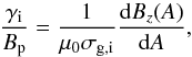
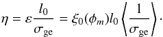
We define the following conductivities:  (40)which resemble
the gyroconductivity introduced by Speiser
(1968). However, in the definition of Speiser’s gyroconductivity only the
Bz component was used.
This component was oriented perpendicular to the antiparallel field lines of the magnetic
neutral sheet, so that particles within the neutral sheet are gyrating around
Bz and therefore
encounter an electric field (in their own frame of
reference, see Lyons & Speiser 1985). Since, in our case, there
exists no magnetic neutral sheet, we have to use
(40)which resemble
the gyroconductivity introduced by Speiser
(1968). However, in the definition of Speiser’s gyroconductivity only the
Bz component was used.
This component was oriented perpendicular to the antiparallel field lines of the magnetic
neutral sheet, so that particles within the neutral sheet are gyrating around
Bz and therefore
encounter an electric field (in their own frame of
reference, see Lyons & Speiser 1985). Since, in our case, there
exists no magnetic neutral sheet, we have to use  for the corresponding magnetic field, and the particles gyrate around its field lines.
By inserting the definition of the gyroconductivities (Eq. (40)) into the equation of the current (Eq. (34)), we obtain  (41)from which
ξ can in
principle be calculated. In the situation in which βi =
βe ≠ γi =
γe, the resistance ξ results in
(41)from which
ξ can in
principle be calculated. In the situation in which βi =
βe ≠ γi =
γe, the resistance ξ results in
 (42)This scenario is very
unlikely, as it implies that the electrons (owing to their much smaller mass) would run
away from the ions because the electric field accelerates the lighter electrons much more
strongly than the heavy ions. Hence, the configuration would not reach a stationary state.
(42)This scenario is very
unlikely, as it implies that the electrons (owing to their much smaller mass) would run
away from the ions because the electric field accelerates the lighter electrons much more
strongly than the heavy ions. Hence, the configuration would not reach a stationary state.
For the ions to achieve about the same acceleration as the electrons, the total electric
field encountered by the electrons must be negligible compared with the total field
encountered by the ions. Therefore, if we set in Eq. (41) βi ≫ βe and
γi ≫
γe, which is physically more reasonable,
we obtain the following expression for ξ:
 (43)With
the help of this formula we can estimate the Speiser-like resistivity.
(43)With
the help of this formula we can estimate the Speiser-like resistivity.
To ensure that the poloidal component of Ei is
the dominating one, we demand that 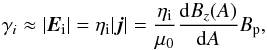 (44)where the term on the
right-hand side again refers to the current of the MHD picture. Then, Eq. (44) can be rewritten in the form
(44)where the term on the
right-hand side again refers to the current of the MHD picture. Then, Eq. (44) can be rewritten in the form
 (45)where we used the
identity for the resistivity
(45)where we used the
identity for the resistivity  .
Because we have no precise information about the acceleration terms from MHD theory, it is
physically reasonable to request that the acceleration should be field-aligned, that is,
.
Because we have no precise information about the acceleration terms from MHD theory, it is
physically reasonable to request that the acceleration should be field-aligned, that is,
 (46)We now define
 (47)Therefore,
ξ can be
written as
(47)Therefore,
ξ can be
written as  where
we introduced the parameter ε2 =
σg,i/σg,e.
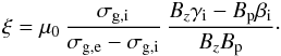
Because according to Eq. (24)
where
we introduced the parameter ε2 =
σg,i/σg,e.
Because according to Eq. (24)
 , the resistivity has the form
 (51)Owing to the
quasi-neutrality ε2
≈ 1, which means that η ~ 1
/σg,e =
ηe. Consequently, the total resistivity,
and therefore also the function ξ, is related to the gyroresistivity of the
electrons.
(51)Owing to the
quasi-neutrality ε2
≈ 1, which means that η ~ 1
/σg,e =
ηe. Consequently, the total resistivity,
and therefore also the function ξ, is related to the gyroresistivity of the
electrons.
The resistivity (hence the Ohmic heating) depends on the chosen geometry and on the constraint of only having almost field-aligned forces. To keep the resistivity finite, a deviation from exact neutrality (=quasi-neutrality) is required. To keep this deviation small, the field-aligned forces have to be chosen appropriately, so that in the expression of the resistivity, Eq. (51), the “geometrical” term (1 − ε1), which describes the deviation from field-aligned acceleration, compensates for the denominator (1 − ε2), which describes the deviation from perfect neutrality. This compensation should be made in such a way that η is bounded, implying that ε is on the order of unity or at least bounded by some finite value. This guarantees that the resistivity η can be computed at all. A second important criterion why ε should be bounded and on the order of unity comes from calculating the energies of the charged particles. Because according to Eq. (21) the electric potential results from integrating over the resistance ξ, the magnitude of the voltage that the electric particles can achieve is largely determined by the value of ε. If ε were much higher than unity, the energies of the particles would approach the relativistic regime, in which the theory is not valid anymore.
In the following section we present one example with representative physical parameters and simplified magnetic field configuration.
3. Results
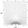 |
Fig. 1 Field line projection onto the poloidal plane. |
The scenario under investigation assumes that the field is almost relaxed, which supports
the assumption of a potential field for the poloidal component of the field (here: the
x and
y components
in the translational invariant magnetic field configuration). We concentrate on a small
region around the footpoint of a solar arcade structure with dimensions 3 Mm × 3 Mm. This domain was chosen to avoid
bipolar magnetic field structures with high plasma β that contain current sheets
with a component of the current in z-direction. We represent the magnetic field
configuration with a 2D dipole superimposed on a homogeneous, monopolar field component in
y-direction.
This results in a dome-like structure at the bottom and an X-point separatrix on top. This
configuration is achieved by expanding the complex magnetic vector potential,
 ,
in a Laurent series of the form
,
in a Laurent series of the form 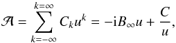 (52)with the complex
constants Ck of which only those
for the homogeneous component (C1 = −iB∞)
and the dipole component (C-1 = i | C |) are
considered, while all others are set to zero. The constant | C | in the latter is given
by | C | =
B∞R2, where
R corresponds
to the height y
above the dipole at which the poloidal field vanishes. This height marks the location of the
magnetic null point. The choice of the constants guarantees that the asymptotical boundary
condition, namely B( | u | → ∞) =
B∞ey,
is fulfilled. The field lines of the configuration are displayed in Fig. 1. Because this figure shows the projection of the field
lines onto the poloidal plane, it represents the two cases before and after the magnetic
shear is applied that results from the shear flow (see Eq. (11)). To compute these field lines, we chose values appropriate for the
solar corona. Magnetic field determinations are usually complicated and values obtained from
observations at different locations and wavelength regions range from about 10-3 T to 10-1 T (see, e.g., Lin et al. 2000; Brosius & White 2006; Caspi & Lin
2010). We adopted a mean value of the magnetic field of B∞ =
10-2 T and for the height R = 1 Mm. The contour lines
of the magnetic potential φm are depicted in Fig.
2. They are everywhere perpendicular to the magnetic
field lines.
(52)with the complex
constants Ck of which only those
for the homogeneous component (C1 = −iB∞)
and the dipole component (C-1 = i | C |) are
considered, while all others are set to zero. The constant | C | in the latter is given
by | C | =
B∞R2, where
R corresponds
to the height y
above the dipole at which the poloidal field vanishes. This height marks the location of the
magnetic null point. The choice of the constants guarantees that the asymptotical boundary
condition, namely B( | u | → ∞) =
B∞ey,
is fulfilled. The field lines of the configuration are displayed in Fig. 1. Because this figure shows the projection of the field
lines onto the poloidal plane, it represents the two cases before and after the magnetic
shear is applied that results from the shear flow (see Eq. (11)). To compute these field lines, we chose values appropriate for the
solar corona. Magnetic field determinations are usually complicated and values obtained from
observations at different locations and wavelength regions range from about 10-3 T to 10-1 T (see, e.g., Lin et al. 2000; Brosius & White 2006; Caspi & Lin
2010). We adopted a mean value of the magnetic field of B∞ =
10-2 T and for the height R = 1 Mm. The contour lines
of the magnetic potential φm are depicted in Fig.
2. They are everywhere perpendicular to the magnetic
field lines.
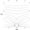 |
Fig. 2 Contour lines of the magnetic potential. |
The only effective electric field component that can act as a particle accelerator is the
component parallel to the magnetic field. From the representations of the total magnetic
field (Eq. (13)) and the electric field (Eq.
(23)), the parallel component of the
electric field, E∥, results in
 (53)To maximize E∥, it is
essential to choose a rather small magnetic shear component1. However, the magnetic shear should neither be constant nor zero, because this
would imply a current-free field.
(53)To maximize E∥, it is
essential to choose a rather small magnetic shear component1. However, the magnetic shear should neither be constant nor zero, because this
would imply a current-free field.
The crucial term in computing E∥ is the resistance function
ξ. This
function was defined in Eq. (20) to be a
pure funtion of φm. However, as was
shown in Eq. (50), it contains the
derivative of the magnetic shear component, which is a pure function of A. Hence, we need to find a
reasonable approach for , that allows us to determine the
profile of the function ξ(φm).
According to Eq. (50), ξ is given by  (54)Because we request that
the null point of the poloidal magnetic field is also a null point of the complete magnetic
field, Bz(A =
0) has to vanish. A Taylor expansion of Bz(A)
around the null point hence delivers that in the lowest order of A the magnetic shear
component must have the form
(54)Because we request that
the null point of the poloidal magnetic field is also a null point of the complete magnetic
field, Bz(A =
0) has to vanish. A Taylor expansion of Bz(A)
around the null point hence delivers that in the lowest order of A the magnetic shear
component must have the form  (55)because the contour line
A = 0 is the
separatrix. The shape of the magnetic shear component Bz(A) is
shown in Fig. 3. For the computation we chose a value
for the constant in Eq. (55) of
5×10⁻⁸ m-1 to guarantee that | Bz |
< | Bp |. Given the
highest values of ~
10-3 T in the dipole region, the magnetic shear component is
still very small compared with the superimposed poloidal field (B∞ ~
10-2 T).
(55)because the contour line
A = 0 is the
separatrix. The shape of the magnetic shear component Bz(A) is
shown in Fig. 3. For the computation we chose a value
for the constant in Eq. (55) of
5×10⁻⁸ m-1 to guarantee that | Bz |
< | Bp |. Given the
highest values of ~
10-3 T in the dipole region, the magnetic shear component is
still very small compared with the superimposed poloidal field (B∞ ~
10-2 T).
 |
Fig. 3 Spatial distribution of the magnetic shear component. |
The absolute value of the electric current over the considered domain and the corresponding contour plot are shown in Fig. 4, while the individual contributions in x and y direction are shown in Fig. 5. The current flows along the poloidal field direction, that is, in x- and y-direction. Above the dipole region, here for y> 1 Mm, the total current is very low and approaches a constant value. This is visible in the top right panel of Fig. 4, which shows the total current at large distances, and also from the contour plots, which show the increasing separation of the contour lines with increasing distance from the dipole. In the region of the dipole field, the x-component of the current flows into the positive x-direction in the left part of the dome, and oppositely in the right part. The dominant component of the current is the y component, which diverges close to the pole.
 |
Fig. 4 Total current of the stationary state (top) and its contour lines (bottom). For better visualization the panels to the right display the behavior of the current beyond the dipole region, i.e. at far distances. |
 |
Fig. 5 Electric current of the stationary state. Displayed are the x-component (left) and the y-component (right). |
The region around the null point can be “evacuated”, for example, after an ejection of a flux rope. This means that the total magnetic field and the electron density both approach zero. Outside the null point region, where the magnetic field saturates, we assume that the density saturates as well. Therefore, the term | B | / (nee) = | B∞ | / (ne,∞e) can be assumed to be approximately constant. The chosen values for B∞ and ne,∞ can be adjusted to typical coronal values. We emphasize, however, that not every arbitrary combination of | B | and ne will successfully deliver a strong enough resistivity or electric field. The last unknown in the function ξ, which we define as the profile function ξ0(φm), is the term ε. This term is requested to cover the φm dependence of the resistance ξ. For our test calculations we set | ξ0(φm) | ≤ 1 to guarantee the quasi-neutrality condition and the physical significance, in other words, to keep the ε-term bounded as physical requirement.
For different choices of and Bp,
we must also recognize that the magnetic shear has to be chosen such that
 results in a reasonable value for
the amplitude of the energy per charge unit, the voltage φe(φm).
Otherwise the ε-term has to be adjusted, which changes the constraint
|
ξ0(φm) | ≤
1. The implication of a lower value of Bp and/or a higher
value of the density has then to be compensated for either by an enhancement of
or an increase of ε, which causes enhanced
deviation from neutrality relative to the deviation from the field-aligned acceleration.
This would not cause problems, because the deviation from neutrality will usually be
extremly small, such that any relative change or fluctuation of the ε1-parameter will
be larger. For one single profile function with
results in a reasonable value for
the amplitude of the energy per charge unit, the voltage φe(φm).
Otherwise the ε-term has to be adjusted, which changes the constraint
|
ξ0(φm) | ≤
1. The implication of a lower value of Bp and/or a higher
value of the density has then to be compensated for either by an enhancement of
or an increase of ε, which causes enhanced
deviation from neutrality relative to the deviation from the field-aligned acceleration.
This would not cause problems, because the deviation from neutrality will usually be
extremly small, such that any relative change or fluctuation of the ε1-parameter will
be larger. For one single profile function with  , where l0 is a typical
lengthscale for the shear that we set to 2 ×
107 m, we can write
, where l0 is a typical
lengthscale for the shear that we set to 2 ×
107 m, we can write
 (56)However, our approach
allows defining multiple sites for acceleration and heating via a fragmented resistivity,
(56)However, our approach
allows defining multiple sites for acceleration and heating via a fragmented resistivity,
 (57)The sign of the individual
ξ0,i can be either
positive or negative, and accordingly, the direction of acceleration can change at each of
these multiple acceleration sites.
(57)The sign of the individual
ξ0,i can be either
positive or negative, and accordingly, the direction of acceleration can change at each of
these multiple acceleration sites.
In the current investigation, we focused on an example using one single, “monolithic”
profile of the form 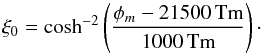 (58)From observations (e.g.,
Aschwanden & Benz 1997), electron densities in acceleration sites of
solar flares of (0.6−10)
× 1015
m-3 were measured.
As acceleration regions are usually regions where the electron density is preferentially low
(see, e.g., Aschwanden
2002), we fixed it in our model at ne,∞ = 1014
m-3. Figure 6 shows the resulting resistivity, η, in the computed domain,
which for our chosen simplifications is directly proportional to the total resistance
ξ. The
resistivity shows a kinked wall-like structure above the null point region and a ring-shaped
wall below. This is easily understood from inspecting Eq. (54) and the plot of the contour lines of the magnetic potential (Fig.
2). Because the resistivity is basically the same
function as the profile function ξ0, which itself is only a function of the
magnetic potential φm while all other
terms in Eq. (54) are constant, the
resistivity reaches a maximum where ξ0 has a maximum. As the isocontours of
the function φm have two disjoint
branches at the numerical value of φm = 21 500 Tm, every
global function of φm also has two
disjoint isocountours with the same isocontour value.
(58)From observations (e.g.,
Aschwanden & Benz 1997), electron densities in acceleration sites of
solar flares of (0.6−10)
× 1015
m-3 were measured.
As acceleration regions are usually regions where the electron density is preferentially low
(see, e.g., Aschwanden
2002), we fixed it in our model at ne,∞ = 1014
m-3. Figure 6 shows the resulting resistivity, η, in the computed domain,
which for our chosen simplifications is directly proportional to the total resistance
ξ. The
resistivity shows a kinked wall-like structure above the null point region and a ring-shaped
wall below. This is easily understood from inspecting Eq. (54) and the plot of the contour lines of the magnetic potential (Fig.
2). Because the resistivity is basically the same
function as the profile function ξ0, which itself is only a function of the
magnetic potential φm while all other
terms in Eq. (54) are constant, the
resistivity reaches a maximum where ξ0 has a maximum. As the isocontours of
the function φm have two disjoint
branches at the numerical value of φm = 21 500 Tm, every
global function of φm also has two
disjoint isocountours with the same isocontour value.
The resulting spatial variation of E∥ is shown in Fig. 7. This parallel component of the electric field is almost identical to the total electric field (see Fig. 8). Particles are strongest affected, that is, heated and accelerated, in the domains in which E∥ is high. These are also the regions of highest voltage, as is obvious from Fig. 9. Because according to the mathematical frame of our theory we are able to superimpose different ξ0 profiles, it is possible to construct fragmented structures of multiple walls, which provide many regions of enhanced electric field that are suitable for consecutive heating (and acceleration) of the particles.
4. Discussion and conclusions
A parallel electric field component tends to accelerate particles, especially electrons, out of the thermal distribution, resulting in so-called runaway particles. However, the acceleration only works efficiently if the parallel electric field component is sufficiently high. Otherwise, the energy gained from the electric field will mainly be dissipated into heat by dynamical friction (in a collisionless plasma as in our case) or collisions (in a collisional plasma). Such dissipation connected with Ohmic heating has been shown to be a reliable mechanism for coronal heating based on detailed 3D numerical MHD simulations (see, e.g., Bingert & Peter 2011; Bourdin et al. 2013).
To measure the effectivity of particle acceleration, the parallel electric field strength
E∥
is typically compared with the Dreicer electric field ED(Dreicer 1960). This Dreicer field is clearly defined in collisional plasmas,
where it is on the order of 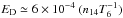 V m-1, where n14 is the plasma
density in units of 1014 m-3, and T6 is the temperature in units of
106 K. For
collisionless plasmas, the definition of the Dreicer field is less straightforward and has
only been considered for the anomalous resistivity, where the effective collision frequency
is defined, and was found to be 4 to 6 orders of magnitude higher than the classical Spitzer
value (e.g.,
Papadopoulos 1977; Priest & Forbes 2000).
V m-1, where n14 is the plasma
density in units of 1014 m-3, and T6 is the temperature in units of
106 K. For
collisionless plasmas, the definition of the Dreicer field is less straightforward and has
only been considered for the anomalous resistivity, where the effective collision frequency
is defined, and was found to be 4 to 6 orders of magnitude higher than the classical Spitzer
value (e.g.,
Papadopoulos 1977; Priest & Forbes 2000).
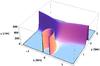 |
Fig. 6 Spatial distribution of the resistivity η. |
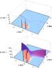 |
Fig. 7 Parallel electric field component. For better visualization, the bottom panel shows E∥ cut off at a numerical value of 0.3 V/m. |
In our collisionless scenario with Speiser-like (particle inertia) resistivity, a proper
definition of a corresponding Dreicer field fails. Because of the nonlinearity between the
electric field and the current, no effective collision frequency can be computed. Instead,
there exists a nonlinear interplay between the particle movement and their relative drift
and the geometrical structure of the electromagnetic field. Therefore the resistivity does
not depend linearly on a collision frequency (as is the case for the Spitzer and the
anomalous or turbulent resistivity), so that the effective Dreicer field ED∗
cannot simply be calculated via the relation ED∗ =
(η∗/η0)ED
given by Norman &
Smith (1978): In the classical view, the current density j =
ED/η0
is fixed, so that any enhancement of η0 causes an increase of the Dreicer
field. The inertia-based resistivity approach does not allow fixing the current density and
simultaneously enlarging the resistivity without enlarging magnetic field and/or reducing
parameterically the density. This is caused by the definition of the differential electric
potential ξ.
The relation obtained by Norman &
Smith (1978) assumes that the change of the resistivity has no influence on the
current density. This is not the case in our scenario where, in general, the resistivity and
the current density depend parametrically on the differential magnetic shear. Furthermore,
Eq. (24) implies that raising the current by
raising the differential magnetic shear  alone, the noncollisional
resistivity even decreases. The assumption that the current is (approximately) fixed implies
that
alone, the noncollisional
resistivity even decreases. The assumption that the current is (approximately) fixed implies
that  constant2. Every parametrical increase of
  and
Bz leads to a decrease of
Bp
and therefore also of the electric field, because | E | ∝
ξBp. Thus
and
Bz leads to a decrease of
Bp
and therefore also of the electric field, because | E | ∝
ξBp. Thus
 leads to a slight
enhancement (if |
Bz/Bp
| ≲ 1) of ξ, but the price is the total decrease of the electric
field. Increasing Bp alone would lead to an increase of
η and of the
electric field.
leads to a slight
enhancement (if |
Bz/Bp
| ≲ 1) of ξ, but the price is the total decrease of the electric
field. Increasing Bp alone would lead to an increase of
η and of the
electric field.
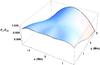 |
Fig. 8 Ratio of the parallel and total electric fields. |
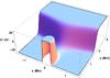 |
Fig. 9 Spatial distribution of the voltage. |
One might doubt the role of the εi-terms, of course, but they mainly depend on a geometrical factor, where the deviation from quasi-neutrality must correspond to the deviation from field-aligned acceleration to avoid the decoupling of ξ from the two-species system and guarantee the regularity of ξ (bounded value for the electric field and ξ). This term can in principle change the Speiser-like resistivity by order(s) of magnitude, but, as it must be bounded and has to compensate for the smallness of the deviation from field-aligned acceleration, it only has a marginal influence in our approach.
Hence we have no clear diagnostics at hand to estimate the efficiency of particle acceleration. However, according to our initial conditions and requirements (quasi-neutrality, low drift velocity), no strong acceleration of the bulk particles is expected. Instead, only particles in the high-energy tail of the Maxwellian distribution might be affected because for them even a (very) small fraction of the classical Dreicer electric field is sufficient to accelerate them into runaway particles. However, as the resulting electric field in our model is almost completely parallel to the magnetic field, the particles will experience some acceleration along the field lines. Our whole scenario is based on a slight charge separation and a separate treatment of ions and electrons. An ultimate investigation of these processes requires a proper two-fluid analysis.
Although a full two-fluid analysis is beyond the scope of the current investigation, we can
use the two-fluid perspective and the parameters from our model calculations to compute
averaged velocities of the particles in the straight field-line region3 and estimate from this the highest and lowest energy of the bulk
particles in our plasma model. The electric current density in the straight field-line
region is approximately 3 ×
10-4 A m-2 (see Fig. 4). On
the other hand, the current density in the two-fluid picture is connected to the particle
velocities via j =
niqvi −
neeve.
We assume that the ion velocity should be on the order of the bulk velocity, which is
 ,
where B ≈
10-2 T, and ρ ≈
nimp.
Furthermore, the absolute values of the charges of the electron and ion (i.e., in our case
protons) are equal, and the electron and ion densities are approximately equal because of
quasi-neutrality and have (in our model) a value of ni ≈ ne
= 1014 m-3. This results in an electron velocity of ve ≈ 1 / 3
MA × 108 m s-1. If we assume a minimum Alfvén
Mach number of 0.1 and a maximum of ≲
1, the energy of the bulk electrons is between about 1 keV and 10 keV. In contrast, typical coronal values of
the thermal energy of electrons for temperatures in the range 106 K to 107 K are about 0.1 keV or 1 keV.
,
where B ≈
10-2 T, and ρ ≈
nimp.
Furthermore, the absolute values of the charges of the electron and ion (i.e., in our case
protons) are equal, and the electron and ion densities are approximately equal because of
quasi-neutrality and have (in our model) a value of ni ≈ ne
= 1014 m-3. This results in an electron velocity of ve ≈ 1 / 3
MA × 108 m s-1. If we assume a minimum Alfvén
Mach number of 0.1 and a maximum of ≲
1, the energy of the bulk electrons is between about 1 keV and 10 keV. In contrast, typical coronal values of
the thermal energy of electrons for temperatures in the range 106 K to 107 K are about 0.1 keV or 1 keV.
Based on our sheared potential field model, we achieve voltage values (~10 kV) in agreement with observed X-ray
emission from solar flares (e.g.,
with RHESSI, see Aschwanden 2002; Önel & Mann 2009). This voltage value
can be up to an order of magnitude higher if we allow for a higher value of
. However, the highest voltage is
not high enough to produce the highly energetic particles with energies in MeV and even GeV
range (see, e.g., Hurford et al.
2003). Our calculated example basically produces a single wall or sheet (see
Fig. 7), meaning that particles are practically
accelerated only once. For a sustained acceleration of the bulk, multiple walls are
necessary. In the frame of our anlysis, a high number of consecutive walls, even with
different amplitudes, can be obtained if we allow that either Bz(A) or
the differential electric potential ξ or both are functions with a high spatial variation
(fragmented). Under such considerations the voltage will also be fragmented, producing
numerous solitary-wave-shaped “walls”. The existence of such multiple fractal structures
within the electromagnetic field allows repetetive acceleration (or decelaration) processes
to very high energies as well. However, for a spatially variable magnetic shear component
the φm dependence of the
resistance ξ
cannot be expressed in a simple way, and the null point of the initial poloidal potential
field is not necessarily conserved anymore. The pure linear dependence of Bz(A) on
A considered
in the presented example is a severe restriction. Better models in which Bz(A) can be adjusted to constraints and boundary conditions require that in general σg,e must also explicitly depend on A and φm, which complicates the analysis. Furthermore, for a more consistent investigation the generalized Ohm’s law needs to be considered, and for this the MHD should be replaced by a real two-fluid approach.
Nevertheless, the great advantage of our MHD model is that it explicitly identifies the current caused by the drift between the accelerated particles with the current caused by the magnetic shear component. It is thus a valuable and self-consistent approach in the frame of nonideal MHD, which automatically incorporates the nonlinear electromagnetic feedback of the particles, which is ignored in the usual test particle approach.
The Bz component is not really restricted to low values as every Bz = Bz(A) produces an equilibrium because of the noncanonical transformation method. But low values of the shear component compared with the main poloidal component of the field are of advantage to maximize E∥, to justify the assumption of quasi-neutrality, and to fulfill the dominance of the poloidal over the z-component of the total electric field of the ions (see Eq. (47)).
As Bp is a function of φm and A in general, it is not possible to keep the current fixed.
The region, where the asymptotic boundary condition is reached.
Acknowledgments
We thank the anonymous referee for useful comments and suggestions on the draft. This research made use of the NASA Astrophysics Data System (ADS). D.H.N. and M.K. acknowledge financial support from GA ČR under grant numbers 13-24782 and P209/12/0103, respectively. The Astronomical Institute Ondřejov is supported by the project RVO:67985815.
References
- Aschwanden, M. J. 2002, Space Sci. Rev., 101, 1 [NASA ADS] [CrossRef] [Google Scholar]
- Aschwanden, M. J., & Benz, A. O. 1997, ApJ, 480, 825 [NASA ADS] [CrossRef] [Google Scholar]
- Bingert, S., & Peter, H. 2011, A&A, 530, A112 [NASA ADS] [CrossRef] [EDP Sciences] [Google Scholar]
- Birn, J., Artemyev, A. V., Baker, D. N., et al. 2012, Space Sci. Rev., 173, 49 [Google Scholar]
- Bourdin, P.-A., Bingert, S., & Peter, H. 2013, A&A, 555, A123 [NASA ADS] [CrossRef] [EDP Sciences] [Google Scholar]
- Brosius, J. W., & White, S. M. 2006, ApJ, 641, L69 [NASA ADS] [CrossRef] [Google Scholar]
- Brown, J. C., Turkmani, R., Kontar, E. P., MacKinnon, A. L., & Vlahos, L. 2009, A&A, 508, 993 [NASA ADS] [CrossRef] [EDP Sciences] [Google Scholar]
- Caspi, A., & Lin, R. P. 2010, ApJ, 725, L161 [NASA ADS] [CrossRef] [Google Scholar]
- Drake, J. F., Opher, M., Swisdak, M., & Chamoun, J. N. 2010, ApJ, 709, 963 [NASA ADS] [CrossRef] [Google Scholar]
- Dreicer, H. 1960, Phys. Rev., 117, 329 [NASA ADS] [CrossRef] [Google Scholar]
- Dungey, J. W., & Speiser, T. W. 1969, Planet. Space Sci., 17, 1285 [NASA ADS] [CrossRef] [Google Scholar]
- Gebhardt, U., & Kiessling, M. 1992, Phys. Fluids B, 4, 1689 [NASA ADS] [CrossRef] [Google Scholar]
- Giacalone, J., Drake, J. F., & Jokipii, J. R. 2012, Space Sci. Rev., 173, 283 [NASA ADS] [CrossRef] [Google Scholar]
- Grad, H., & Hogan, J. 1970, Phys. Rev. Lett., 24, 1337 [NASA ADS] [CrossRef] [Google Scholar]
- Hurford, G. J., Schwartz, R. A., Krucker, S., et al. 2003, ApJ, 595, L77 [Google Scholar]
- Kane, S. R. 1974, in Coronal Disturbances, ed. G. A. Newkirk, IAU Symp., 57, 105 [Google Scholar]
- Karlický, M., & Bárta, M. 2007, Adv. Space Res., 39, 1427 [NASA ADS] [CrossRef] [Google Scholar]
- Karlický, M., & Kosugi, T. 2004, A&A, 419, 1159 [NASA ADS] [CrossRef] [EDP Sciences] [Google Scholar]
- Lazarian, A., & Vishniac, E. T. 1999, ApJ, 517, 700 [NASA ADS] [CrossRef] [Google Scholar]
- Leake, J. E., Linton, M. G., & Török, T. 2013, ApJ, 778, 99 [NASA ADS] [CrossRef] [Google Scholar]
- Lin, H., Penn, M. J., & Tomczyk, S. 2000, ApJ, 541, L83 [NASA ADS] [CrossRef] [Google Scholar]
- Lyons, L. R., & Speiser, T. W. 1985, J. Geophys. Res., 90, 8543 [NASA ADS] [CrossRef] [Google Scholar]
- Miller, J. A. 1998, Space Sci. Rev., 86, 79 [NASA ADS] [CrossRef] [Google Scholar]
- Nickeler, D. H., & Wiegelmann, T. 2010, Ann. Geophys., 28, 1523 [NASA ADS] [CrossRef] [Google Scholar]
- Nickeler, D. H., & Wiegelmann, T. 2012, Ann. Geophys., 30, 545 [NASA ADS] [CrossRef] [Google Scholar]
- Nickeler, D. H., Goedbloed, J. P., & Fahr, H.-J. 2006, A&A, 454, 797 [NASA ADS] [CrossRef] [EDP Sciences] [Google Scholar]
- Nickeler, D. H., Karlický, M., Wiegelmann, T., & Kraus, M. 2013, A&A, 556, A61 [NASA ADS] [CrossRef] [EDP Sciences] [Google Scholar]
- Norman, C. A., & Smith, R. A. 1978, A&A, 68, 145 [NASA ADS] [Google Scholar]
- Önel, H., & Mann, G. 2009, Central Eur. Astrophys. Bull., 33, 141 [NASA ADS] [Google Scholar]
- Papadopoulos, K. 1977, Rev. Geophys. Space Phys., 15, 113 [NASA ADS] [CrossRef] [Google Scholar]
- Petrie, G. J. D., & Neukirch, T. 1999, Geophys. Astrophys. Fluid Dyn., 91, 269 [Google Scholar]
- Priest, E., & Forbes, T. 2000, Magnetic Reconnection [Google Scholar]
- Speiser, T. W. 1968, in Earth’s Particles and Fields, ed. B. M. McCormac, 393 [Google Scholar]
- Speiser, T. W. 1970, Planet. Space Sci., 18, 613 [NASA ADS] [CrossRef] [Google Scholar]
- Throumoulopoulos, G. N. 1998, J. Plasma Phys., 59, 303 [NASA ADS] [CrossRef] [Google Scholar]
- Throumoulopoulos, G. N., & Tasso, H. 2000, J. Plasma Phys., 64, 601 [NASA ADS] [CrossRef] [Google Scholar]
- Wang, H. 1992, Sol. Phys., 140, 85 [NASA ADS] [CrossRef] [Google Scholar]
- Zharkova, V. V., Arzner, K., Benz, A. O., et al. 2011, Space Sci. Rev., 159, 357 [NASA ADS] [CrossRef] [Google Scholar]
All Figures
|
Fig. 1 Field line projection onto the poloidal plane. |
| In the text | |
|
Fig. 2 Contour lines of the magnetic potential. |
| In the text | |
|
Fig. 3 Spatial distribution of the magnetic shear component. |
| In the text | |
|
Fig. 4 Total current of the stationary state (top) and its contour lines (bottom). For better visualization the panels to the right display the behavior of the current beyond the dipole region, i.e. at far distances. |
| In the text | |
|
Fig. 5 Electric current of the stationary state. Displayed are the x-component (left) and the y-component (right). |
| In the text | |
|
Fig. 6 Spatial distribution of the resistivity η. |
| In the text | |
|
Fig. 7 Parallel electric field component. For better visualization, the bottom panel shows E∥ cut off at a numerical value of 0.3 V/m. |
| In the text | |
|
Fig. 8 Ratio of the parallel and total electric fields. |
| In the text | |
|
Fig. 9 Spatial distribution of the voltage. |
| In the text | |
Current usage metrics show cumulative count of Article Views (full-text article views including HTML views, PDF and ePub downloads, according to the available data) and Abstracts Views on Vision4Press platform.
Data correspond to usage on the plateform after 2015. The current usage metrics is available 48-96 hours after online publication and is updated daily on week days.
Initial download of the metrics may take a while.