| Issue |
A&A
Volume 569, September 2014
|
|
|---|---|---|
| Article Number | A90 | |
| Number of page(s) | 9 | |
| Section | Cosmology (including clusters of galaxies) | |
| DOI | https://doi.org/10.1051/0004-6361/201423758 | |
| Published online | 29 September 2014 | |
First experimental constraints on the disformally coupled Galileon model
1
CEA, Centre de Saclay, Irfu/SPP,
91191
Gif-sur-Yvette,
France
e-mail:
jeremy.neveu@cea.fr
2
LPNHE, Université Pierre et Marie Curie, Université Paris Diderot,
CNRS-IN2P3, 4 place
Jussieu, 75252
Paris Cedex 5,
France
3
Center for Astrophysics and Space Astronomy, University of
Colorado, Boulder,
CO
80309-0389,
USA
4
Laboratoire de Physique Théorique d’Orsay, Bâtiment 210,
Université Paris-Sud 11, 91405
Orsay Cedex,
France
Received:
4
March
2014
Accepted:
7
August
2014
Aims. The Galileon model is a modified gravity model that can explain the late-time accelerated expansion of the Universe. In a previous work, we derived experimental constraints on the Galileon model with no explicit coupling to matter and showed that this model agrees with the most recent cosmological data. In the context of braneworld constructions or massive gravity, the Galileon model exhibits a disformal coupling to matter, which we study in this paper.
Methods. After comparing our constraints on the uncoupled model with recent studies, we extend the analysis framework to the disformally coupled Galileon model and derive the first experimental constraints on that coupling, using precise measurements of cosmological distances and the growth rate of cosmic structures.
Results. In the uncoupled case, with updated data, we still observe a low tension between the constraints set by growth data and those from distances. In the disformally coupled Galileon model, we obtain better agreement with data and favour a non-zero disformal coupling to matter at the 2.5σ level. This gives an interesting hint of the possible braneworld origin of Galileon theory.
Key words: dark energy / cosmology: observations / supernovae: general
© ESO, 2014
1. Introduction
Dark energy remains one of the deepest mysteries of cosmology today. Even though it has been fifteen years since the discovery of dark energy (Riess et al. 1998; Perlmutter et al. 1999), its fundamental nature remains unknown. Adding a cosmological constant (Λ) to Einstein’s general relativity is the simplest way to account for this observation, and leads to remarkable agreement with all cosmological data so far (see e.g. Planck Collaboration XVI 2014). However, the cosmological constant requires considerable fine-tuning to explain current observations and motivates the quest for alternative explanations of the nature of dark energy.
Modified gravity models aim to provide such an explanation. The Galileon theory, first proposed by Nicolis et al. (2009) involves a scalar field, hereafter called π, whose equation of motion must be of second order and invariant under a Galilean shift symmetry ∂μπ → ∂μπ + bμ, where bμ is a constant vector. This symmetry was first identified as an interesting property in the DGP model (Dvali et al. 2000). Nicolis et al. (2009) derived the five possible Lagrangian terms for the field π, which were then formulated in a covariant formalism by Deffayet et al. (2009a) and Deffayet et al. (2009b).
This model forms a subclass of general tensor-scalar theories involving only up to second-order derivatives originally found by Horndeski (1974). Later, Galileon theory was also found to be the non-relativistic limit of numerous broader theories, such as massive gravity (de Rham & Gabadadze 2010) or brane constructions (de Rham & Tolley 2010; Hinterbichler et al. 2010; Acoleyen & Doorsselaere 2011). Braneworld approaches give a deeper theoretical basis to Galileon theories. The usual and simple construction involves a 3+1 dimensional brane, our Universe, embedded in a higher dimensional bulk. The Galileon field π can be interpreted as the brane transverse position in the bulk, and the Galilean symmetry appears naturally as a remnant of the broken space-time symmetries of the bulk (Hinterbichler et al. 2010). The Galilean symmetry is then no longer imposed as a principle of construction, but is a consequence of space-time geometry.
Models that modify general relativity have to alter gravity only at cosmological scales in
order to agree with the solar system tests of gravity (see e.g. Will 2006). The Galileon field can be coupled to matter either explicitly
or through a coupling induced by its temporal variation (Babichev & Esposito-Farese 2013). This leads to a so-called fifth force
that by definition modifies gravity around massive objects like the Sun. But the non-linear
Lagrangians of the Galileon theory ensure that this fifth force is screened near massive
objects in case of an explicit coupling of the form  (where
 is the trace
of the matter energy-momentum tensor, c0 a dimensionless parameter, and
MP
the Planck mass) or in the case of an induced coupling. This is called the Vainshtein effect
(Vainshtein 1972 and Babichev & Deffayet 2013 for a modern introduction). The fifth
force is thus negligible with respect to general relativity within a certain radius from a
massive object, that depends on the object mass and Galileon parameters (Vainshtein 1972; Nicolis
et al. 2009; Brax et al. 2011).
is the trace
of the matter energy-momentum tensor, c0 a dimensionless parameter, and
MP
the Planck mass) or in the case of an induced coupling. This is called the Vainshtein effect
(Vainshtein 1972 and Babichev & Deffayet 2013 for a modern introduction). The fifth
force is thus negligible with respect to general relativity within a certain radius from a
massive object, that depends on the object mass and Galileon parameters (Vainshtein 1972; Nicolis
et al. 2009; Brax et al. 2011).
Braneworld constructions and massive gravity models give rise to an explicit disformal
coupling to matter of the form ~
∂μπ∂νπTμν.
As shown, for example, in Brax et al. (2012), this
coupling does not induce a fifth force on massive objects since it does not apply to
non-relativistic objects when the scalar field is static. In a cosmological context, the
scalar field π
evolves with time but the fifth force introduced by the disformal coupling to matter can be
masked thanks to a new screening mechanism (Koivisto
2012; Zumalacarregui 2013). However, the
disformal coupling still plays a role in the field cosmological evolution, which makes this
kind of Galileon model interesting to compare with cosmological data. The action of the
model is 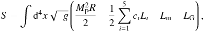 (1)with Lm the matter
Lagrangian, R
the Ricci scalar, and g the determinant of the metric. The cis are the Galileon model
dimensionless parameters weighting different covariant Galileon Lagrangians Li (Deffayet et al. 2009a):
(1)with Lm the matter
Lagrangian, R
the Ricci scalar, and g the determinant of the metric. The cis are the Galileon model
dimensionless parameters weighting different covariant Galileon Lagrangians Li (Deffayet et al. 2009a):
![\begin{eqnarray} L_1 &= & M^3\pi,\quad L_2=\pi_{;\mu}\pi^{;\mu},\quad L_3=(\pi_{;\mu}\pi^{;\mu})(\square \pi)/M^3, \notag \\ L_4 &= & (\pi_{;\mu}\pi^{;\mu})\left[ 2(\square \pi)^2 - 2 \pi_{;\mu\nu}\pi^{;\mu\nu} - R(\pi_{;\mu}\pi^{;\mu})/2 \right]/M^6, \notag \\ L_5 &= & (\pi_{;\mu}\pi^{;\mu}) \left[ (\square \pi)^3 - 3(\square \pi) \pi_{;\mu\nu}\pi^{;\mu\nu} +2\pi_{;\mu}\ ^{;\nu}\pi_{;\nu}^{\ ;\rho}\pi_{;\rho}^{\ ;\mu} \right. \notag \\ && \left. -6 \pi_{;\mu}\pi^{;\mu\nu}\pi^{;\rho}G_{\nu\rho}\right]/M^9, \end{eqnarray}](/articles/aa/full_html/2014/09/aa23758-14/aa23758-14-eq17.png) (2)where
M is a mass
parameter defined as
(2)where
M is a mass
parameter defined as  with H0 the Hubble
parameter current value. LG is the disformal coupling to matter:
with H0 the Hubble
parameter current value. LG is the disformal coupling to matter:
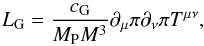 (3)where cG is
dimensionless. Interestingly, Babichev et al. (2011)
showed that c0 ≲
10-2 by comparing local time variation measurements of the
Newton constant GN in the Lunar Laser Ranging experiments,
to predictions derived in the Galileon theory with the Vainshtein mechanism accounted for
and boundary conditions set by the cosmological evolution. In the more general context of
scalar field theories, the disformal coupling has been recently constrained in particle
physics using Large Hadron Collider data (Brax &
Burrage 2014; CMS Collaboration 2014). Thus
the disformal coupling should be the first explicit Galileon coupling to look at considering
the actual existing constraints.
(3)where cG is
dimensionless. Interestingly, Babichev et al. (2011)
showed that c0 ≲
10-2 by comparing local time variation measurements of the
Newton constant GN in the Lunar Laser Ranging experiments,
to predictions derived in the Galileon theory with the Vainshtein mechanism accounted for
and boundary conditions set by the cosmological evolution. In the more general context of
scalar field theories, the disformal coupling has been recently constrained in particle
physics using Large Hadron Collider data (Brax &
Burrage 2014; CMS Collaboration 2014). Thus
the disformal coupling should be the first explicit Galileon coupling to look at considering
the actual existing constraints.
The uncoupled Galileon model (cG = 0) has already been constrained by
observational cosmological data in Appleby & Linder
(2012b), Okada et al. (2013), Nesseris et al. (2010), and more recently in Neveu et al. (2013, hereafter N13) and Barreia et al. (2013a, hereafter B13a). In N13, we introduced a new parametrisation of the model and
developed a likelihood analysis method to constrain the Galileon parameters independently of
initial conditions on the π field. The unknown initial condition for the Galileon
field was absorbed into the original ci parameters to form new
parameters  defined by
  , where
x0
encodes the initial condition for the Galileon field. The same methodology was adopted here,
and we refer the interested reader to N13 for more
details.
, where
x0
encodes the initial condition for the Galileon field. The same methodology was adopted here,
and we refer the interested reader to N13 for more
details.
Same datasets were used for baryonic acoustic oscillations (BAO; Beutler et al. 2011; Padmanabhan et al. 2012; Sánchez et al. 2012), and for growth of structure joint measurements1 of fσ8(z) and the Alcock-Paczynski parameter F(z), mainly from Percival et al. (2004), Blake et al. (2011), Beutler et al. (2012), Samushia et al. (2012a), Reid et al. (2012). For the cosmic microwave background (CMB), we updated our analysis to use the WMAP9 distance priors (Hinshaw et al. 2012) instead of the WMAP7 ones (Komatsu et al. 2011). Concerning type Ia supernovae (SNe Ia), we also updated our sample from the high-quality data of the SuperNova Legacy Survey (SNLS) collaboration (Guy et al. 2010; Conley et al. 2011; Sullivan et al. 2011) to the recent sample published jointly by the SNLS and Sloan Digital Sky Survey (SDSS) collaborations (Betoule et al. 2014), which we will refer to as the joint light-curve analysis (JLA) sample in the following.
Interesting constraints on the uncoupled Galileon model using the full CMB power spectrum were published in B13a, with a different methodology. In the following, we show that the results from both studies agree. However, in our study we used growth data, despite our using a linearised version of the theory, while B13a preferred not to use those data until the Galileon non-linearities responsible for the Vainshtein effect are precisely studied. We include a discussion on that important point in this paper.
Section 2 describes our updated datasets. Section 3 provides an update of the constraints on the uncoupled Galileon model, using WMAP9 and JLA data, and a comparison with B13a results. Section 4 gives constraints on the disformally coupled Galileon model derived from the same dataset. Section 5 discusses these results and their implications, as well as the state of the art of growth rate of structure modelling in Galileon theory. We conclude in Sect. 6.
2. Updated datasets
2.1. Updated CMB data
WMAP distance priors.
The new CMB distance priors and their covariance matrix from WMAP9 (Hinshaw et al. 2012) were used as CMB constraints (see Table 1). No major improvements are expected as the distance priors uncertainties are not significantly decreased in the WMAP9 release. Planck results would be very competitive but the Planck Collaboration did not publish similar distance priors independent of the Λ cold dark matter (ΛCDM) model2.
In N13 as well as in this work, we followed the
prescriptions of Komatsu et al. (2009) for the use
of WMAP distance priors to derive cosmological constraints. In particular, they recommend
a minimisation procedure of the h value when comparing predictions to observables.
Because of the rich Galileon phase space to explore, we added in N13 a Gaussian prior on H0 to help the program converge, centred
on the Riess et al. (2011) measurement. Since then,
the Planck Collaboration published their results and showed a disagreement between their
ΛCDM fit and the Riess et al. (2011) measurement for H0. In order to
measure the impact of that measurement on our results, we repeated the study without the
H0 prior. Results on e.g.
 and
and
 are presented in Table 2. When removing the
H0 prior, best-fit values and the
minimised h
value do not change drastically. The χ2 at the marginalised values decreased
from 2.1 to 0.7, indicating that there is a small tension between the WMAP9 distance
priors and H0 measurement. The check was also
performed in the disformally coupled Galileon and ΛCDM models, and led to similar results. As
a consequence, we decided to remove the H0 prior in the following.
are presented in Table 2. When removing the
H0 prior, best-fit values and the
minimised h
value do not change drastically. The χ2 at the marginalised values decreased
from 2.1 to 0.7, indicating that there is a small tension between the WMAP9 distance
priors and H0 measurement. The check was also
performed in the disformally coupled Galileon and ΛCDM models, and led to similar results. As
a consequence, we decided to remove the H0 prior in the following.
Impact of the H0 Gaussian prior on constraints on two of the uncoupled Galileon model parameters using BAO+WMAP9 data.
2.2. Updated SN Ia sample
Cosmological constraints on the uncoupled Galileon model from the SNLS3 and JLA samples.
In N13, the SNLS3 sample from Conley et al. (2011) was used. The JLA sample recently
released by the SNLS and SDSS collaborations benefit from reduced calibration systematic
uncertainties and combine the full SDSS-II spectroscopically-confirmed SN Ia sample with
the SNLS3 sample. While the SNLS3 sample contain 472 supernovae whose parameters were
determined using a combination of the SALT2 and SiFTO light-curve fitters, 740 supernovae
are present in the final JLA sample, measured using SALT2 only. The impact of the new
calibration and change in the light-curve fitter shifted the best fit
value for a
flat ΛCDM model from
0.228 ± 0.038 to
0.295 ± 0.034
(1.8σ
drift, see Betoule et al. 2013 and Sect. 6.4 of
Betoule et al. 2014, for more details). This new
value is now more consistent with the Planck measurement (Planck Collaboration XVI 2014).
Both samples were used to derive constraints on the Galileon model parameters. Results are presented in Table 3 and illustrated in Fig. 1. Usually, one should fit and marginalise over the two nuisance parameters α and β, which describe the SN Ia variability in stretch and colour (Astier et al. 2006; Guy et al. 2010; Conley et al. 2011). However, in N13 it was shown that for the Galileon model we can keep α and β fixed to their marginalised values in the ΛCDM model. In this study, we thus took directly the fitted α and β value from N13 for the SNLS3 sample and from Betoule et al. (2014) for the JLA sample3.
Using the new JLA sample, we observe a 1σ increase of the best fit
value, as
expected when considering the reported drift for the ΛCDM model in Betoule et al. (2014). Smaller changes are observed for the
parameters.
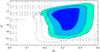 |
Fig. 1 Experimental constraints on |
2.3. Updated growth data computation
From the Planck Collaboration, we used the new value
 (Planck Collaboration XVI 2014) to normalise our growth rate
predictions, as we are able to remove the ΛCDM dependence for that observable. We recall that to compute
fσ8(z)
predictions in the Galileon model we assume that the value of σ8 is equal in
the Galileon and ΛCDM models
at the decoupling redshift z∗. This is a reasonable assumption as
we showed in our previous paper that the Galileon energy density is very subdominant at
that time for most of the allowed set of parameters. The uncertainty on
(Planck Collaboration XVI 2014) to normalise our growth rate
predictions, as we are able to remove the ΛCDM dependence for that observable. We recall that to compute
fσ8(z)
predictions in the Galileon model we assume that the value of σ8 is equal in
the Galileon and ΛCDM models
at the decoupling redshift z∗. This is a reasonable assumption as
we showed in our previous paper that the Galileon energy density is very subdominant at
that time for most of the allowed set of parameters. The uncertainty on
 was propagated in our error
budget. We still used growth data with the same caveats as mentioned in N13 and B13a,
which we discuss further in Sect. 5.
was propagated in our error
budget. We still used growth data with the same caveats as mentioned in N13 and B13a,
which we discuss further in Sect. 5.
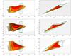 |
Fig. 2 Experimental constraints on the uncoupled Galileon model from growth data (red) and from JLA+WMAP9+BAO combined constraints (dashed). The filled dark, medium and light coloured contours enclose 68.3, 95.4 and 99.7% of the probability, respectively. Dark dotted regions correspond to scenarios rejected by theoretical constraints. |
3. Uncoupled Galileon model
In this section, we derived new experimental constraints on the
parameters of the uncoupled Galileon model following the same methodology as in N13 with updated data.
3.1. New experimental constraints
Uncoupled Galileon model best-fit values from different data samples.
Results using all probes are presented in Fig. 2, and Table 4. With the SNLS3 data, the updated WMAP9 priors and the Planck σ8 value improved only marginally the constraints and χ2 values of the Galileon model compared to our previous results using WMAP7 (see lines 5 and 6 in Table 4). However, because this dataset is now more consistent with that used in B13a, we can compare our two sets of results, obtained with different methodologies, which we do in the next section.
Finally, using the JLA sample does not improve the
uncertainty
but decreases our uncertainties on the
Galileon parameters. This sample will be used to constrain the disformally coupled model
in Sect. 4.
3.2. Comparison with B13a
B13a recently provided constraints on the Galileon parameters, using the full WMAP9 CMB power spectrum whereas we used only distance priors. The rest of their dataset is identical to ours (except for one BAO measurement, which should not impact the result).
They used a different method to get rid of the degeneracies inherent to the original
ci parametrisation, and
derived constraints on  ratios. Their method of computing the initial conditions is also different and more
complex. Despite the different methodologies and parametrisations, the comparison of
parameter ratios is possible as we have
ratios. Their method of computing the initial conditions is also different and more
complex. Despite the different methodologies and parametrisations, the comparison of
parameter ratios is possible as we have
 (4)This can give an
interesting insight into the impact of the use of the full CMB power spectrum, and of
different methodologies. Results using SNe Ia, CMB and BAO data (no growth data) in both
works are compared in Table 5. Both results are
fully compatible even if our methodologies are different. Our
values and
uncertainties are comparable, but the B13a best-fit
uncertainties are about ten times smaller than ours thanks to the use of the full CMB
spectrum.
(4)This can give an
interesting insight into the impact of the use of the full CMB power spectrum, and of
different methodologies. Results using SNe Ia, CMB and BAO data (no growth data) in both
works are compared in Table 5. Both results are
fully compatible even if our methodologies are different. Our
values and
uncertainties are comparable, but the B13a best-fit
uncertainties are about ten times smaller than ours thanks to the use of the full CMB
spectrum.
This can be understood as follows. Distance priors are derived from the first acoustic peak only, which are measurements at the decoupling redshift where the Galileon field is subdominant. But, as shown in Barreia et al. (2012), in the Galileon theory the low-l CMB power spectrum is very sensitive to the model parameters, because this part of the spectrum is affected by late-time dark energy through the integrated Sachs-Wolfe (ISW) effect. The Galileon model is thus severely constrained by this part of the spectrum, and can even provide a better fit to the CMB power spectrum than the ΛCDM model thanks to a better agreement in the low-l region (B13a).
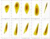 |
Fig. 3 Combined constraints on the disformally coupled Galileon model from growth data combined with JLA+BAO+WMAP9 data. The filled dark, medium and light yellow contours enclose 68.3, 95.4 and 99.7% of the probability, respectively. Dark dotted regions correspond to scenarios rejected by theoretical constraints. |
4. Galileon model disformally coupled to matter
4.1. Hypothesis
In Appleby & Linder (2012a), a disformal coupling LG between the matter and the Galileon field was proposed, motivated by extra-dimension considerations. LG introduces a new parameter to constrain, cG. This kind of coupling naturally arises in the decoupling limit of massive gravity (see de Rham & Heisenberg 2011). It also automatically arises when dealing with a fluctuating 3+1 brane in a D = 4 + n dimensional bulk, when matter lives exclusively in the brane. This disformal coupling has already been studied in scalar field theories other than the Galileon model as reported in Brax et al. (2012).
In particular, Brax et al. (2012) and Andrews et al. (2013) showed that this kind of coupling has no gravitational effect on massive objects, and thus fulfils the Solar System gravity tests. However, it couples to photons and can play a role in gravitational lensing (see Wyman 2011).
In this work, as in N13, we used the same
cosmological and perturbation equations as in Appleby
& Linder (2012a), but the cG parameter was renormalised as
 (5)with
x0 defined in N13.
(5)with
x0 defined in N13.
Introducing this coupling did not require us to modify the methodology of N13, but we had to assume that this coupling between matter and the Galileon field did not change the thermodynamics of the primordial plasma before decoupling. Indeed, if such a coupling is assumed, energy transfers should happen between the scalar field and the primordial plasma. In particular the disformal term leads to interactions between photons and the π field. However, as shown in N13, the uncoupled Galileon field is negligible during the radiation era in most scenarios, which limits the potential impact of the Galileon before the decoupling. We assumed that this is also the case here, in order to give a first glance at this interesting coupling.
4.2. Results
Disformally coupled Galileon model best-fit values from growth rate measurements combined with JLA+BAO+WMAP9 data.
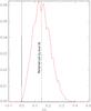 |
Fig. 4
|
The results using type Ia SNe, CMB, BAO measurements and growth data are presented in Figs. 3, 4, and Table 6.
As in the uncoupled case, the best fit lies
around 0.27. The
and  best fit values changed slightly, but are still compatible at one sigma with their best
fit values in the uncoupled case, which is not the case for
best fit values changed slightly, but are still compatible at one sigma with their best
fit values in the uncoupled case, which is not the case for
 .
As shown in Table 6,
.
As shown in Table 6,
 is excluded at the
2.5σ level,
and as a consequence, the final χ2 is better than in the coupled case.
is excluded at the
2.5σ level,
and as a consequence, the final χ2 is better than in the coupled case.
The probability density function obtained for  (Fig. 4) shows clearly that a non-zero best fit value
is preferred for this parameter, at the 2.5σ level. Note that when using distances only,
this result still holds but at the 1.4σ level. The disformally coupled Galileon model
appears thus in better agreement with data than the uncoupled model. This may support an
extra-dimension origin for the Galileon theory as this coupling is unavoidable in such
constructions.
(Fig. 4) shows clearly that a non-zero best fit value
is preferred for this parameter, at the 2.5σ level. Note that when using distances only,
this result still holds but at the 1.4σ level. The disformally coupled Galileon model
appears thus in better agreement with data than the uncoupled model. This may support an
extra-dimension origin for the Galileon theory as this coupling is unavoidable in such
constructions.
4.3. Implications beyond cosmology
The parameter space explored in this work was defined by theoretical conditions that ensure that our cosmological solution is free of ghosts and instability problems (see Sect. 2.5 of N13).
Recently, Berezhiani et al. (2011) and Koyama et al. (2013) pointed out that some Galileon-like theories may lead to ghost instabilities in solutions inside massive objects, when a disformal coupling is involved. One should note, however, that our model does not fall exactly in their discussion. However, following a reasoning similar to that in Berezhiani et al. (2011), we checked that our model may avoid the ghost problem thanks to a compensation between the fifth Lagrangian term L5 and LG. Thus, our best-fit result is likely to be valid also inside massive objects, but deriving an explicit no-ghost condition to ensure that this is indeed the case is beyond the scope of this paper, since we restricted to cosmological solutions only.
5. Discussion
5.1. Non-linearities in the Galileon model
In N13, we provided some caveats about the use of growth data when comparing with predictions of a linearised Galileon model. In particular, we stressed that:
-
non-linear models of growth of structures were used to extract measurements from data, whereas here only the linear perturbation theory was used to describe matter perturbation evolution;
-
the non-linearities of the Galileon field itself were also neglected in the perturbed equations while they play a key role in the Vainshtein effect, in particular to restore general relativity close to massive objects.
In particular for the latter point, below a certain distance from a massive object, called the Vainshtein radius, Galileon gravity is supposed to vanish with respect to general relativity. At small scales, the growth of structures is then identical in both models. But the Vainshtein radius depends on the Galileon parameters and on the massive object properties, and hence it is difficult to know which scales are affected by Galileon gravity in general.
However, recent progress on the inclusion of non-linearities (both from the Galileon field and from matter evolution) has been made using N-body simulations of structure evolution in Galileon gravity (Barreia et al. 2013b,c; Li et al. 2013). Matter power spectra were computed at the non-linear level for different Galileon models. In Barreia et al. (2013b), the cubic Galileon model (i.e. with c4 = c5 = 0) was studied. It was shown that, for scales k between 0.1 and 0.4 h Mpc-1 (the ones encompassed in our growth data measurements), the deviation between a linear and a non-linear Galileon model is at most of ≈ 5%, and only at redshifts below 0.2. The authors then studied a quartic Galileon model in Li et al. (2013). Important deviations appear between the linear and the non-linear model for the velocity divergence power spectrum (the one of interest for redshift space distortions), but the authors recommended more precise simulations before drawing firm conclusions on that point. Finally, Barreia et al. (2013c) showed that the quintic Galileon model (the one we are using) has non-physical solutions in high matter density regions and that prevented them from doing simulations in that case. According to the authors, these non-physical solutions are either inherent to the Galileon model itself, or due to the approximations made in their non-linear computations. Further work has to be done on the non-linear modelling of the quintic Galileon gravity to make reliable predictions for the growth of structures.
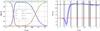 |
Fig. 5 Evolution of the Ωi(z)
(left) and of w(z)
(right, solid curve) for the best-fit disformally coupled Galileon
model from all data (last row of Table 6). In
the left plot, dashed lines correspond to our ΛCDM best-fit values. Differences in
the radiation era are only due to different best-fit values of h. In the
right plot, the shaded area was obtained varying the
|
5.2. Comparison with the ΛCDM model
χ2s at marginalised values for different models and different datasets.
The best-fit coupled Galileon scenario still mimics a ΛCDM model with the three periods of radiation, matter, and dark energy domination, with an evolving dark energy equation of state parameter w(z) (see Fig. 5). This feature is not different from what we obtained in the uncoupled case.
Table 7 presents the χ2 values of the two Galileon models and the ΛCDM one (see also Fig. 6). With only distances, the three models reach the same level of agreement with data. When adding growth data, the increase in χ2 is higher for the Galileon models, as a result of a higher tension between growth and distance probes (see also Figs. 2 and 6). But the difference in χ2 with respect to the ΛCDM model is not stringent. As in our previous work, we can conclude that the Galileon model is not significantly disfavoured by current data compared to the ΛCDM model, and is a good alternative to model dark energy.
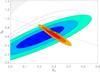 |
Fig. 6 Experimental constraints on the ΛCDM model from JLA data (blue), growth data (red), BAO+WMAP9 data (green), and all data combined (yellow). Purple dashed contours stand for the ΛCDM constraints using SNLS3 data only (combining SIFTO and SALT2 supernova parameters). The black dashed line indicates the flatness condition Ωm + ΩΛ = 1. |
6. Conclusion
We have compared the uncoupled and disformally coupled Galileon models to the most recent
cosmological data, using the methodology from our previous work (N13). An update of the uncoupled Galileon model experimental constraints
using WMAP9 {la,R,z∗}
constraints was derived jointly with the new JLA SN Ia sample, BAO measurements, and growth
data with the Alcock-Paczynski effect taken into account. The σ8(z =
0) value used to compute the growth of structure observable was also
updated to the Planck Collaboration XVI (2014) value.
The JLA sample allowed us to derive better constraints on the
parameters. When we kept the SNLS3 sample, our constraints did not change significantly, but
led to an interesting comparison with the Galileon best-fit values published in B13a. They used the full WMAP9 power spectrum to derive
their constraints, and thus brought tighter constraints, but both best-fit scenarios agree.
This validates both methodologies despite their differences. As expected, WMAP9 distance
priors are less constraining than the full CMB spectrum but provide a simpler and faster way
to derive constraints on the Galileon model.
We provided the first experimental constraints on the disformal coupling parameter in the framework of the Galileon model. This coupling between matter and the Galileon field is natural when building the theory from massive gravity or extra-dimension considerations. Our final χ2’s are comparable to the one obtained for the ΛCDM model. Galileon theories are thus competitive to explain the nature of dark energy. We also showed that a null disformal coupling to matter is excluded at the 2.5σ level when using growth data, and at the 1.4σ level when using distances only. This gives some interesting clues, from experimental data, on the possible extra-dimension origin of Galileon theories.
Better constraints would be possible including the ISW effect as shown in B13a. The galaxy velocity field could also be a decisive probe to test modified gravity theories, as advocated in (Zu 2013; Hellwing et al. 2014). However, this probe would require to have a correct modelling of the Galileon model non-linearities. Interestingly, the disformal coupling couples to light and thus can have an impact on gravitational lensing (Wyman 2011). Lensing experiments such as LSST (Ivezic et al. 2008) or the future satellite Euclid (Laureijs et al. 2011), or laboratory tests with light shining through a wall experiments (Brax et al. 2012) can provide more data to constrain this interesting coupling. CMB spectral distortion studies (Brax et al. 2013) will also give further insight into the braneworld origin of the Galileon theory.
Note however that recently an independent group proposed a derivation of the distance priors from the Planck+WP+lensing power spectrum (Wang 2013).
References
- Acoleyen, K., & Doorsselaere, J. 2011, Phys. Rev. D., 83, 084025 [NASA ADS] [CrossRef] [Google Scholar]
- Astier, P., Guy, J., Regnault, N., et al. 2006, A&A, 447, 31 [NASA ADS] [CrossRef] [EDP Sciences] [Google Scholar]
- Anderson, L., Aubourg, E., Bailey, S., et al. 2013, MNRAS, 427, 3435 [NASA ADS] [CrossRef] [Google Scholar]
- Andrews., M., Chu, Y. Z., & Trodden, M. 2013, Phys. Rev. D, 88, 84028 [NASA ADS] [CrossRef] [Google Scholar]
- Appleby, S. A., & Linder, E. 2012a, JCAP, 1203, 44 [Google Scholar]
- Appleby, S. A., & Linder, E. 2012b, JCAP, 08, 26 [NASA ADS] [CrossRef] [Google Scholar]
- Barreira, A., Li, B., Baugh, C. M., et al. 2012, Phys. Rev. D, 86, 124016 [NASA ADS] [CrossRef] [Google Scholar]
- Barreira, A., Li, B., Baugh, C. M., et al. 2013a, Phys. Rev. D, 87, 103511 (B13a) [NASA ADS] [CrossRef] [Google Scholar]
- Barreira, A., Li, B., Hellwing, W. A., et al. 2013b, JCAP, 20, 027 [NASA ADS] [CrossRef] [Google Scholar]
- Barreira, A., Li, B., Baugh, C. M., et al. 2013c, JCAP, 11, 012 [Google Scholar]
- Babichev, E., & Esposito-Farese, G. 2013, Phys. Rev. D, 87, 044032 [NASA ADS] [CrossRef] [Google Scholar]
- Babichev, E., & Deffayet, C. 2013, Class. Quantum. Grav, 30, 184001 [Google Scholar]
- Babichev, E., Deffayet, C., & Esposito-Farese, G. 2011, Phys. Rev. Lett., 107, 251102 [NASA ADS] [CrossRef] [PubMed] [Google Scholar]
- Berezhiani, L., Chkareuli, G., & Gabadadze, G. 2013, Phys. Rev. D, 88, 124020 [NASA ADS] [CrossRef] [Google Scholar]
- Betoule, M., Marriner, J., Regnault, N., et al. 2013, A&A, 552, A124 [NASA ADS] [CrossRef] [EDP Sciences] [Google Scholar]
- Betoule, M., Kessler, R., Guy, J., et al. 2014, A&A, 568, A22 [NASA ADS] [CrossRef] [EDP Sciences] [Google Scholar]
- Beutler, F., Blake, C., Colless, M., et al. 2011, MNRAS, 416, 3017 [NASA ADS] [CrossRef] [Google Scholar]
- Beutler, F., Blake, C., Colless, M., et al. 2012, MNRAS, 423, 3430 [NASA ADS] [CrossRef] [Google Scholar]
- Blake, C., Glazebrook, K., Davis, T. M., et al. 2011, MNRAS, 418, 1725 [NASA ADS] [CrossRef] [Google Scholar]
- Brax, P., & Burrage, C. 2014 [arXiv:1407.1861] [Google Scholar]
- Brax, P., Burrage, C., & Davis, A.-C. 2011, JCAP, 1109, 020 [NASA ADS] [CrossRef] [Google Scholar]
- Brax, P., Burrage, C., & Davis, A.-C. 2012, JCAP, 1210, 016 [NASA ADS] [CrossRef] [Google Scholar]
- Brax, P., Burrage, C., Davis, A.-C., et al. 2013, JCAP, 11, 001 [NASA ADS] [CrossRef] [Google Scholar]
- CMS Collaboration 2014, CMS-PAS-EXO-12-047 [Google Scholar]
- Conley, A., Guy, J., Sullivan, M., et al. 2011, ApJS, 192, 1 [NASA ADS] [CrossRef] [EDP Sciences] [Google Scholar]
- De Felice, A., & Tsujikawa, S. 2010, Living. Rev. Lett., 13, 3 [NASA ADS] [Google Scholar]
- Deffayet, C., Esposito-Farese, G., & Vikman, A. 2009a, Phys. Rev. D, 79, 084003 [NASA ADS] [CrossRef] [Google Scholar]
- Deffayet, C., Deser, S., & Esposito-Farese, G. 2009b, Phys. Rev. D, 80, 064015 [NASA ADS] [CrossRef] [Google Scholar]
- Dvali, G. R., Gabadadze, G., & Porrati, M. 2000, Phys. Lett. B, 485, 208 [NASA ADS] [CrossRef] [MathSciNet] [Google Scholar]
- Guy, J., Sullivan, M., Conley, A., et al. 2010, A&A, 523, A7 [NASA ADS] [CrossRef] [EDP Sciences] [Google Scholar]
- Hellwing, W. A., Barreira, A., Frenk, K. S., et al. 2014, Phys. Rev. Lett., 112, 221102 [NASA ADS] [CrossRef] [Google Scholar]
- Hinshaw, G., Larson, D., Komatsu, E., et al. 2012, ApJS, 208, 19 [Google Scholar]
- Hinterbichler, K., Trodden, M., & Wesley, D. 2010, Phys. Rev. D., 82, 124018 [NASA ADS] [CrossRef] [Google Scholar]
- Horndeski, G. W. 1974, Int. J. Theor. Phys., 10, 363-384 [CrossRef] [MathSciNet] [Google Scholar]
- Ivezic, Z., Tyson, J., Acosta, E., et al. 2008, unpublished [arXiv:0805.2366] [Google Scholar]
- Komatsu, E., Dunkley, J., Nolta, M. R., et al. 2009, ApJS, 180, 330 [NASA ADS] [CrossRef] [Google Scholar]
- Komatsu, E., Smith, K. M., Dunkley, J., et al. 2011, ApJS, 192, 18 [NASA ADS] [CrossRef] [Google Scholar]
- Koivisto, T. S., Mota, D. F., & Zumalacarregui, M., 2012, Phys. Rev. Lett., 109, 241102 [NASA ADS] [CrossRef] [Google Scholar]
- Koyama, K., Niz, G., & Tasinato, G. 2013, Phys. Rev. D, 88, 021502 [NASA ADS] [CrossRef] [Google Scholar]
- Laureijs, R., Amiaux, J., Arduini, S., et al. 2011, unpublished [arXiv:1110.3193] [Google Scholar]
- Li, B., Barreira, A., Baugh, C. M., et al. 2013, JCAP, 11, 012. [NASA ADS] [CrossRef] [Google Scholar]
- Nesseris, S., De Felice, A., & Tsujikawa, S. 2010, Phys. Rev. D, 82, 124054 [NASA ADS] [CrossRef] [Google Scholar]
- Neveu, J., Ruhlmann-Kleider, V., & Conley, A. 2013, A&A, 555, A53 (N13) [NASA ADS] [CrossRef] [EDP Sciences] [Google Scholar]
- Nicolis, A., Rattazzi, R., & Trincherini, E. 2009, Phys. Rev. D, 79, 064036 [NASA ADS] [CrossRef] [MathSciNet] [Google Scholar]
- Okada, H., Totani, T., & Tsujikawa, S. 2013, Phys. Rev. D, 87, 103002 [Google Scholar]
- Padmanabhan, N., Xu, X., Eisenstein, D. J., et al. 2012, MNRAS, 427, 2132 [NASA ADS] [CrossRef] [MathSciNet] [Google Scholar]
- Perlmutter, S., Aldering, G., Goldhaber, G., et al. 1999, ApJ, 517, 565 [NASA ADS] [CrossRef] [Google Scholar]
- Percival, W. J., Burkey, D., Heavens, A., et al. 2004, MNRAS, 353, 1201 [NASA ADS] [CrossRef] [Google Scholar]
- de Rham, C., & Gabadadze, G. 2010, Phys. Rev. D., 82, 4 [NASA ADS] [CrossRef] [MathSciNet] [Google Scholar]
- de Rham, C. & Heisenberg, L. 2011, Phys. Rev. D, 84, 043503 [NASA ADS] [CrossRef] [Google Scholar]
- de Rham, C., & Tolley, A. J. 2010, JCAP, 1005, 015 [NASA ADS] [CrossRef] [Google Scholar]
- Planck Collaboration XVI 2014, A&A, in press, DOI: 10.1051/0004-6361/201321591 [Google Scholar]
- Reid, B. A., Samushia, L., White, M., et al. 2012, MNRAS, 426, 2719 [NASA ADS] [CrossRef] [Google Scholar]
- Riess, A. G., Filippenko, A. V., Challis, P., et al. 1998, AJ, 116, 1009 [NASA ADS] [CrossRef] [Google Scholar]
- Riess, A. G., Macri, L., Casertano, S., et al. 2011, ApJ, 730, 119 [NASA ADS] [CrossRef] [Google Scholar]
- Samushia, L., Percival, W. J., & Raccanelli, A. 2012a, MNRAS, 420, 2102 [NASA ADS] [CrossRef] [Google Scholar]
- Sánchez, A. G., Scóccola, C. G., Ross, A. J., et al. 2012, MNRAS, 425, 415 [NASA ADS] [CrossRef] [Google Scholar]
- Sotiriou, T. P., & Faraoni, V. 2010, Rev. Mod. Phys., 82, 451 [NASA ADS] [CrossRef] [MathSciNet] [Google Scholar]
- Sullivan, M., Guy, J., Regnault, N., et al. 2011, ApJ, 737, 102 [NASA ADS] [CrossRef] [Google Scholar]
- Trodden, M., & Hinterbichler, K. 2011, Class. Quant. Grav., 28, 204003 [NASA ADS] [CrossRef] [Google Scholar]
- Vainshtein, A. I. 1972, Phys. Lett. B, 39, 396 [NASA ADS] [CrossRef] [Google Scholar]
- Wang, Y., & Wang, S. 2013, Phys. Rev. D, 88, 043522 [NASA ADS] [CrossRef] [Google Scholar]
- Will, C. M. 2006, Liv. Rev. Relat., 9, 3 [Google Scholar]
- Wyman, M. 2011, Phys. Rev. Lett., 106, 201102 [NASA ADS] [CrossRef] [Google Scholar]
- Zu, Y., Weinberg, D. H., Jennings, E., et al. 2013 [arXiv:1310.6768] [Google Scholar]
- Zumalacarregui, M., Koivisto, T. S., & Mota, D. F. 2013, Phys. Rev. D, 87, 083010 [NASA ADS] [CrossRef] [Google Scholar]
All Tables
Impact of the H0 Gaussian prior on constraints on two of the uncoupled Galileon model parameters using BAO+WMAP9 data.
Cosmological constraints on the uncoupled Galileon model from the SNLS3 and JLA samples.
Disformally coupled Galileon model best-fit values from growth rate measurements combined with JLA+BAO+WMAP9 data.
All Figures
|
Fig. 1 Experimental constraints on |
| In the text | |
|
Fig. 2 Experimental constraints on the uncoupled Galileon model from growth data (red) and from JLA+WMAP9+BAO combined constraints (dashed). The filled dark, medium and light coloured contours enclose 68.3, 95.4 and 99.7% of the probability, respectively. Dark dotted regions correspond to scenarios rejected by theoretical constraints. |
| In the text | |
|
Fig. 3 Combined constraints on the disformally coupled Galileon model from growth data combined with JLA+BAO+WMAP9 data. The filled dark, medium and light yellow contours enclose 68.3, 95.4 and 99.7% of the probability, respectively. Dark dotted regions correspond to scenarios rejected by theoretical constraints. |
| In the text | |
|
Fig. 4
|
| In the text | |
|
Fig. 5 Evolution of the Ωi(z)
(left) and of w(z)
(right, solid curve) for the best-fit disformally coupled Galileon
model from all data (last row of Table 6). In
the left plot, dashed lines correspond to our ΛCDM best-fit values. Differences in
the radiation era are only due to different best-fit values of h. In the
right plot, the shaded area was obtained varying the
|
| In the text | |
|
Fig. 6 Experimental constraints on the ΛCDM model from JLA data (blue), growth data (red), BAO+WMAP9 data (green), and all data combined (yellow). Purple dashed contours stand for the ΛCDM constraints using SNLS3 data only (combining SIFTO and SALT2 supernova parameters). The black dashed line indicates the flatness condition Ωm + ΩΛ = 1. |
| In the text | |
Current usage metrics show cumulative count of Article Views (full-text article views including HTML views, PDF and ePub downloads, according to the available data) and Abstracts Views on Vision4Press platform.
Data correspond to usage on the plateform after 2015. The current usage metrics is available 48-96 hours after online publication and is updated daily on week days.
Initial download of the metrics may take a while.