| Issue |
A&A
Volume 569, September 2014
|
|
|---|---|---|
| Article Number | A114 | |
| Number of page(s) | 8 | |
| Section | Cosmology (including clusters of galaxies) | |
| DOI | https://doi.org/10.1051/0004-6361/201322730 | |
| Published online | 01 October 2014 | |
Relaxation of dark matter halos: how to match observational data?
1
DESY Zeuthen Platanenallee 6,
15738
Zeuthen,
Germany
e-mail:
baushev@gmail.com
2
Institut für Physik und Astronomie, Universität Potsdam,
14476
Potsdam-Golm,
Germany
Received:
23
September
2013
Accepted:
25
June
2014
We show that moderate energy relaxation in the formation of dark matter halos invariably leads to profiles that match those observed in the central regions of galaxies. The density profile of the central region is universal and insensitive to either the seed perturbation shape or the details of the relaxation process. The profile has a central core; the multiplication of the central density by the core radius is almost independent of the halo mass, in accordance with observations. In the core area the density distribution behaves as an Einasto profile with low index (n ~ 0.5); it has an extensive region with ρ ∝ r-2 at larger distances. This is exactly the shape that observations suggest for the central region of galaxies. On the other hand, this shape does not fit the galaxy cluster profiles. A possible explanation of this fact is that the relaxation is violent in the case of galaxy clusters; however, it is not violent enough when galaxies or smaller dark matter structures are considered. We discuss the reasons for this.
Key words: dark matter / Galaxy: structure / Galaxy: formation / astroparticle physics / methods: analytical
© ESO, 2014
1. Introduction
Although the dark matter (DM) component contributes most to the galaxy mass containment, a generally accepted explanation for some observational properties of the galaxy dark matter halos has not been supplied yet. In particular, there is some disagreement regarding the density profile in the center of the halos. Earlier N-body simulation suggested very cuspy profiles with an infinite density in the center (see, e.g., Moore et al. 1999; Neto et al. 2007). For instance, the Navarro-Frenk-White profile (hereafter NFW) behaves as ρ ∝ r-1 in this area. Recent simulations (Stadel et al. 2009; Navarro et al. 2010) favor an Einasto profile with a finite central density, but the obtained Einasto index n is so high (typically n ~ 5−6) that the profile is very steep in the center and may still be called cuspy. Although the simulations mainly model the largest structures of the Universe, such as galaxy clusters (M ~ 1015 M⊙), their results are expected to be valid for smaller objects as well. Moreover, simulations of separate dark matter halos (M ~ 1012 M⊙) have also be performed (see, for instance, the Via Lactea project Diemand et al. 2007).
However, the correct interpretation of the N-body data requires a reliable estimation of the
simulation convergence. The idea of N-body simulations is to substitute real tiny dark
matter particles by heavy test bodies. Since there are fewer bodies, the task becomes
computable. We face a problem, however: the test bodies collide much more effectively than
the original DM particles. The strong encounters with high momentum transfer lead to evident
effects such as kicking of the test particles from the halo. They are avoided in simulations
by softening of the Newtonian potential near the test bodies. However, the gravitational
force is long-acting, and the influence of weak long-distant collisions dominates. In a
nutshell, the gravitational potential of homogeneous dark matter is plain, while the
potential of the test bodies has local potential wells near the bodies, despite of the
softening. This produces unphysical soft scattering of the bodies on each other and so leads
to a collisional relaxation. The process can be described by the Fokker-Planck approximation
(Landau & Lifshitz 1980). The
characteristic time of the collisional relaxation is (Binney
& Tremaine 2008, Eq. (1.32))  , where
v is the
characteristic particle speed at radius r, N(r) is the number of particles
inside r,
lnΛ is the Coulomb logarithm.
The ratio of the system lifetime t0 to τr should be low enough to
guarantee the negligibility of the relaxation. A real halo contains ~1065 particles, hence the collisions are wholly immaterial.
The quantity of test bodies in simulations is incomparably lower. The closer we approach the
halo center, the smaller N(r) and r/v are, and the
shorter is τr. Thus the central
region of the halos is the most problematic for the simulations: the profile inside some
convergence radius rconv may be already corrupted by the
collisions. It is commonly assumed that rconv is defined by a certain value of
t0/τr.
, where
v is the
characteristic particle speed at radius r, N(r) is the number of particles
inside r,
lnΛ is the Coulomb logarithm.
The ratio of the system lifetime t0 to τr should be low enough to
guarantee the negligibility of the relaxation. A real halo contains ~1065 particles, hence the collisions are wholly immaterial.
The quantity of test bodies in simulations is incomparably lower. The closer we approach the
halo center, the smaller N(r) and r/v are, and the
shorter is τr. Thus the central
region of the halos is the most problematic for the simulations: the profile inside some
convergence radius rconv may be already corrupted by the
collisions. It is commonly assumed that rconv is defined by a certain value of
t0/τr.
The commonly-used criterion of the convergence of N-body simulations is the stability of the central density profile (Power et al. 2003). The simulations indeed show that the central NFW-like cusp is formed quite rapidly (t<τr) and then is stable and insensitive to the simulation parameters. However, the convergence criteria obtained with this method are surprisingly optimistic: the cusp is stable at least up to t = 1.7τr and probably much longer (Power et al. 2003). Hayashi et al. (2003) and Klypin et al. (2013) reported that the cusp is stable even at tens of relaxation times and smears out only at t ~ 40τr. The reasons why the collision influence is negligible at a time interval exceeding the relaxation time are not quite clear. Nevertheless, criterion t = 1.7τr (Power et al. 2003) is routinely used in modern simulations (Navarro et al. 2010).
The criteria based on the density profile stability have a weak point, however: the stability does not guarantee the absence of the collisional influence. Considerations based on the Fokker-Planck equation (Evans & Collett 1997; Baushev 2013b) show that an NFW-like profile (ρ ∝ r−β, β ≃ 1) is an attractor: the Fokker-Planck diffusion transforms any reasonable initial distribution into it in a time shorter than τr, and then the cuspy profile should survive much longer than τr, since the Fokker-Planck diffusion is self-compensated in this case. Therefore the cusp is stable and insensitive to the simulation parameters; at t ~ 50τr it is destroyed by higher-order terms of the Boltzmann collision integral, disregarded by the Fokker-Planck approach (Quinlan 1996; Baushev 2013b). This scenario perfectly describes the behavior of real N-body simulations: the NFW-like cusp appears at t<τr, remains stable up to tens of relaxation times, and then is smoothed. However, the shape of the cusp is in this case defined by the test particle collisions, that is, by a purely numerical effect. The only reliable criterion of negligibility of the unphysical collisions is t ≪ τr. This means that rconv is several times larger than predicted by the criterion t = 1.7τr (Power et al. 2003). Thus the criteria based on the profile stability are most likely too optimistic and underestimate the influence of numerical effects. The problem needs further investigation.
Contrary to the simulations, observations show a fairly smooth core in the centers of, at least, galaxy halos (de Blok et al. 2001; de Blok & Bosma 2002; Marchesini et al. 2002; Gentile et al. 2007). Chemin et al. (2011) removed the baryon contribution and found that the dark matter distribution in the central regions of a large array of galaxies may well be fitted by the Einasto profile with a low index (n ≃ 0.5) that corresponds to a cored profile. The central densities of the dwarf spheroidal satellites of the Andromeda galaxy are also low and favor the cored profiles (Tollerud et al. 2012), although the profiles in this case can be modified by the dynamical friction and tidal effects, since the satellites are situated inside the virial radius of the host galaxy. However, recent observations of dwarf spheroidal galaxies also indicate no cusps in their centers (Oh et al. 2011; Governato et al. 2012). This makes attempts to explain the soft cores of the central density profiles by the influence of the baryonic component dubious: the dwarfs contain only a very minor fraction of baryons.
Many galaxies (at least, the spiral ones) show quite an extensive region in their dark matter halo with a ρ ∝ r-2 profile: the region corresponds to a characteristic flat tail in their rotation curves. This feature allowed proving the existence of the dark matter by Rubin et al. (1978). Meanwhile, none of two profiles (Navarro-Frenk-White or Einasto) that are commonly used to fit the halos in the N-body simulations has such a region. Certainly, the current power-law index γ = dlog ρ/ dlog r of both the profiles reaches −2 at some point. However, the index changes continuously in both cases, the point where γ = −2 is marked not, therefore we cannot expect an extensive region with ρ ~ r-2. Of course, the real structure formation is a much more complex process than the simulations, and the origin of the region could be a result of the influence of the baryon component, substructures, galaxy disk, etc. However, the persistence of the isothermal-like shape ρ ~ r-2 in the density profiles of a vast collection of galaxies with very different physical properties (Sofue & Rubin 2001) suggests a more fundamental and more universal physical reason.
Finally, observations indicate that the multiplication of the halo central density
ρc
by the core radius rcore is almost constant for a wide
variety of galaxies, while their physical parameters, including ρc and
rcore apart, change in a rather extensive
range. This effect was first discovered by Kormendy
& Freeman (2004) and then confirmed by several independent observations
(see Salucci et al. 2007; Donato et al. 2009 and references therein). To be able to compare results
obtained using different profile models, we define the core radius rcore as the
radius, at which  (1)Donato et al. (2009) used the Burkert profile (Burkert 1995)
  (2)It is easy to see
that rcore =
rb/ 2. Recently, Donato et al. (2009) found that log (ρcrb) = 2.15 ±
0.2 in units of log (M⊙ pc-2) on the basis of
the co-added rotation curves of ~1000 spiral galaxies, the mass models of individual dwarf irregular and
spiral galaxies of late and early types with high-quality mass profiles, and the
galaxy-galaxy weak-lensing signals from a sample of spiral and elliptical galaxies. They
also showed that the observed kinematics of Local Group dwarf spheroidal galaxies are
consistent with this value as well. The result was obtained for galactic systems belonging
to various Hubble types whose mass profiles have been determined by several independent
methods.
(2)It is easy to see
that rcore =
rb/ 2. Recently, Donato et al. (2009) found that log (ρcrb) = 2.15 ±
0.2 in units of log (M⊙ pc-2) on the basis of
the co-added rotation curves of ~1000 spiral galaxies, the mass models of individual dwarf irregular and
spiral galaxies of late and early types with high-quality mass profiles, and the
galaxy-galaxy weak-lensing signals from a sample of spiral and elliptical galaxies. They
also showed that the observed kinematics of Local Group dwarf spheroidal galaxies are
consistent with this value as well. The result was obtained for galactic systems belonging
to various Hubble types whose mass profiles have been determined by several independent
methods.
The aim of this article is to show that all the above-mentioned features (a cored central
profile, an extended region with a ρ ∝ r-2 profile, and
ρcrcore ≃
const. relationship) appear automatically, if we
assume that the relaxation of the galactic halos during their formation was not violent. The
violent-relaxation scenario, usually leading to a cuspy density profile, was first suggested
by Lynden-Bell (1967) for stellar systems. The idea
of it is that strong small-scale gravitational fields appear during the halo relaxation, and
as a result all the particles completely forget their initial states. Recent N-body simulations (Diemand et al. 2005, 2007; Diemand & Kuhlen 2008) showed
however, that this assumption is probably incorrect, and a significant part of the particles
and subhalos “remember” their initial specific energies
 : they
change quite moderately.
: they
change quite moderately.
There may be several theoretical reasons for the absence of the violent relaxation (Baushev 2014). For instance, the efficiency of the violent relaxation rapidly drops with the growth of the initial radius r of the area under consideration from the center of the object. Even the original paper (Lynden-Bell 1967) reported that the outer regions of the stellar clusters remained unrelaxed. Meanwhile, a dark matter halo originates from a perturbation that was initially linear and, in contrast to the formed structures, had a low density contrast. Consequently, the main contribution to the halo mass was made by the layers with large r, since their volume 4πr2dr dominates. This circumstance impedes the relaxation. Moreover, a significant part of the dark matter gradually accretes onto the already formed halo, when the strong gravitational field inhomogeneities have already disappeared (Wang et al. 2012).
All these reasons allow us to assume that the violent relaxation does not occur, at least, in some types of halos. Hereafter we assume that the relaxation of low-mass halos (Mvir ≲ 1012 M⊙), corresponding to galaxies, is not violent. We assume that the relaxation is moderate in the following sense:
-
1.
The final total specific energy ϵf of most of the particles differsfrom the initial ones ϵi no more than by a factor cvir/ 5
 (3)
(3) -
2.
There can be particles that violate condition (3), but their total mass should be small with respect to the halo mass inside

 (4)The reason for this
limitation will be clear from the subsequent text.
(4)The reason for this
limitation will be clear from the subsequent text.
Here we used the NFW halo concentration cvir. As we will see, the real density profile may significantly differ from the NFW one, if conditions (3)–(4) are true. However, we use cvir because of its popularity and in view of the fact that characteristic values of cvir for various types of astronomical objects are well known. Condition (3) is too strict for galaxy clusters, since their concentrations are low (cvir ~ 3−5). Indeed, even for rather a dense cluster (cvir = 6) Eq. (3) would mean that the energies of almost all the particles change by no more than 20% during the relaxation. The real relaxation is most likely more intensive; perhaps, this is the reason why the galaxy clusters have profiles close to NFW (Okabe et al. 2010).
In contrast, conditions (3) and (4) seem quite soft for galactic halos.
Concentration cvir ≃
12−17 even for the giant Milky Way galaxy and probably much higher for
low-mass galaxies. Consequently, assumption (3) means that the energy of most of the particles changes no more than by a factor
of 3 with respect to the initial
value. This behavior looks quite natural for a collisionless system. Condition (4) is also weak. Indeed, a halo of typical
galactic concentration (cvir ~ 15−20) contains 20−25% of its mass inside
;
this means that condition (4) reduces to the
constraint that the fraction of the particles that changed their energy by more than a
factor of cvir/ 3 ≃ 3 is smaller
than a quarter of the halo mass.
Of course, there is always some dark matter that violates condition (3). For instance, the particles that were in the center of the halo at the very beginning of the collapse, when their velocities (as well as the velocities of other particles) were low. Their energies changed by much more than Eq. (3) during the collapse, even if there was no relaxation at all. Indeed, they remain in the halo center during the collapse, while the gravitational potential of this area deepens by approximately a factor cvir because of the crowding of the matter toward the center. However, the density of these “ancient habitants” of the halo center was comparable with the average DM density of the Universe at the moment of the halo collapse, that is, it was only by a factor ~5 higher than the present-day value. Meanwhile, the central density of the Milky Way is higher by a factor ~3 × 10⁵ than the Universe DM density. Clearly, the “ancient habitants” do yield some density into the DM content of the Galactic center, but the contribution is negligible (~10-5).
To conclude the introductory section, we should emphasize that the moderate relaxation is now no more than a hypothesis. However, as we will see, it leads to quite correct predictions of the central density profiles of galaxies.
In Sect. 2 we discuss the energy evolution of a collapsing dark matter halo and show that the distribution of the formed halo probably has a peculiar form. In Sect. 3 we calculate the density profile corresponding to this distribution. In Sect. 4 we discuss the obtained profile and compare it with observational data. Finally, in Sect. 4, we briefly summarize our results and discuss further implications.
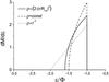 |
Fig. 1 Initial energy spectra |
2. Energy distribution
The assumption of the moderate energy evolution immediately leads to some important
consequences. Hereafter we accept for simplicity that the halo is spherically symmetric. The
present-day dark matter halos were formed from some primordial perturbations that existed in
the early Universe. Initially, the perturbations grew linearly, but then they reached the
nonlinear regime and collapsed. We consider the initial (at the moment when δρ/ρ ≃
1) energy distribution of the particles that later formed the halo. It is
determined by the gravitational field of the initial perturbation, and the closer a particle
was to the center, the lower was its energy. However, the potential well of the initial
perturbation cannot be deep, and the particles cannot have a very low energy, because thy
are lumped in quite a narrow energy interval. Indeed, a trivial Newtonian calculation gives
us the initial energy spectrum for various shapes of initial perturbations (Baushev 2014). We assume for simplicity that the size of
the perturbation at the moment of the collapse is equal to the virial radius of the formed
halo Rvir: these values should be similar in the
very general case (Gorbunov & Rubakov 2010).
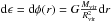
We introduce the virial potential of the halo  .
As an example, we consider the case when the initial density distribution of the
perturbation has the shape ρ ~
r-1 inside Rvir. Then
M(r) =
∫ 4πr2ρdr
=
Mvir(r/Rvir)2
and
.
As an example, we consider the case when the initial density distribution of the
perturbation has the shape ρ ~
r-1 inside Rvir. Then
M(r) =
∫ 4πr2ρdr
=
Mvir(r/Rvir)2
and 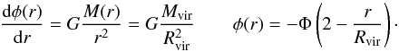 (5)Here we took into account
that φ(Rvir) = −Φ. It follows
from the general cosmological consideration that the initial velocity of the matter may be
thought to be zero without loss of generality (Gorbunov
& Rubakov 2010). Therefore, the specific total energy of a particle is
equal to the specific gravitational energy, that is, to the gravitational potential
ϵ =
φ(r). By dividing
(5)Here we took into account
that φ(Rvir) = −Φ. It follows
from the general cosmological consideration that the initial velocity of the matter may be
thought to be zero without loss of generality (Gorbunov
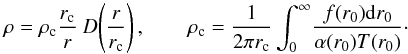
& Rubakov 2010). Therefore, the specific total energy of a particle is
equal to the specific gravitational energy, that is, to the gravitational potential
ϵ =
φ(r). By dividing
 by
by
 , we obtain
  (6)In a similar manner, we can
obtain the initial energy spectra for various forms of initial perturbations (see (Baushev 2014) for details). Distributions
(6)In a similar manner, we can
obtain the initial energy spectra for various forms of initial perturbations (see (Baushev 2014) for details). Distributions
 for three different shapes (
 (solid line), ρ = const. (dash line),
ρ ∝
r-1 (dotted line)) are represented in Fig.
1. In all the cases the spectra are quite similar,
narrow, and strongly concentrated toward ϵ = −Φ. Even an unphysically steep initial
perturbation ρ ~
r-1 contains only particles with
ϵ ∈ [−2Φ; −Φ].
(solid line), ρ = const. (dash line),
ρ ∝
r-1 (dotted line)) are represented in Fig.
1. In all the cases the spectra are quite similar,
narrow, and strongly concentrated toward ϵ = −Φ. Even an unphysically steep initial
perturbation ρ ~
r-1 contains only particles with
ϵ ∈ [−2Φ; −Φ].
We now consider the formed halo. Its gravitational field is stationary. The motion of a
particle in the central gravitational field φ(r) can be explicitly characterized
by two integrals of motion: its specific angular momentum μ ≡ | [ v ×
r ] | and specific energy
 . Instead of ϵ, it is more convenient to
use the apocenter distance of the particle r0, which is the largest distance that the
particle can move away from the center. It is bound with ϵ as
. Instead of ϵ, it is more convenient to
use the apocenter distance of the particle r0, which is the largest distance that the
particle can move away from the center. It is bound with ϵ as
 . We may introduce distribution
function f(r0) of the particles of
the formed halo over r0
. We may introduce distribution
function f(r0) of the particles of
the formed halo over r0 (7)As
we will see, if conditions (3)–(4) are satisfied, f(r0) has a very peculiar
appearance.
(7)As
we will see, if conditions (3)–(4) are satisfied, f(r0) has a very peculiar
appearance.
It is extremely important for our consideration that the potential well of the collapsed
halo is much deeper then the initial one. The depth (i.e., the value of φ(0)) depends on the halo
profile: for the NFW φ(r) ≃ −cvirΦ, if cvir ≫ 1 (Baushev 2012). Although density profiles of real galaxies
are much more complex, φ(r) ≃ −cvirΦ may still be a good approximation. For
instance, we may accept for the Milky Way Mvir =
1012 M⊙, Rvir = 250 kpc,
cvir ≃
15 (Klypin et al. 2002): then
Φ ≃ (130km s)-2.
Meanwhile, the Galaxy escape speed near the solar system unambiguously exceeds
525 km s-1 (Carney & Latham 1987) and may in principle be much higher (650 km s-1 or even higher (Marochnik & Suchkov 1984; Binney & Tremaine 2008)). Accordingly,
 .
.
As we showed, initial energy spectra are very similar for any reasonable shape of the
initial perturbation. We consider for the sake of definiteness an initial perturbation
 , because it seems to be a good
approximation for a real one. We can see in Fig. 1 that
most the particles have ϵ ≃ −Φ, and there are no particles with ϵ< −1.6Φ. Consequently, the particles obeying condition (3) may not have
, because it seems to be a good
approximation for a real one. We can see in Fig. 1 that
most the particles have ϵ ≃ −Φ, and there are no particles with ϵ< −1.6Φ. Consequently, the particles obeying condition (3) may not have
 , and even
the fraction of the particles with
, and even
the fraction of the particles with  is small:
the initial spectrum contains only a few particles with ϵ ≃ −1.6Φ. We estimate
r0, corresponding to a particle with
ϵ = −1.6Φ.
Of course, it depends on the density profile of the halo and on the particle angular
momentum. The influence of the latter factor can be easily taken into account: a nonzero
angular momentum decreases r0 of a particle of a given energy
ϵ, but cannot
decrease it by a factor exceeding 2. Indeed, a particle of given energy ϵ in a given central
gravitational field has the largest r0 if μ = 0, and its orbit is
radial. The ratio of r0 for the radial and the circular cases
is 2 in the instance of the
gravitational field of a point mass. It is easy to see that the ratio can only be lower, if
we consider a distributed density profile instead of a point mass: if the dark matter is
spread, the more compact circular orbit encloses a smaller central mass than in the
point-mass case. Moreover, N-body simulations suggest that the orbits of most of
the particles are elongated (Hansen et al. 2006). In
this case the influence of the angular momentum on r0 is negligible.
is small:
the initial spectrum contains only a few particles with ϵ ≃ −1.6Φ. We estimate
r0, corresponding to a particle with
ϵ = −1.6Φ.
Of course, it depends on the density profile of the halo and on the particle angular
momentum. The influence of the latter factor can be easily taken into account: a nonzero
angular momentum decreases r0 of a particle of a given energy
ϵ, but cannot
decrease it by a factor exceeding 2. Indeed, a particle of given energy ϵ in a given central
gravitational field has the largest r0 if μ = 0, and its orbit is
radial. The ratio of r0 for the radial and the circular cases
is 2 in the instance of the
gravitational field of a point mass. It is easy to see that the ratio can only be lower, if
we consider a distributed density profile instead of a point mass: if the dark matter is
spread, the more compact circular orbit encloses a smaller central mass than in the
point-mass case. Moreover, N-body simulations suggest that the orbits of most of
the particles are elongated (Hansen et al. 2006). In
this case the influence of the angular momentum on r0 is negligible.
A particle of energy has
 in the case of an NFW profile. The potential wells of real galaxies are most likely deeper
than the best-fit NFW predicts (probably because of the influence of the much more
concentrated baryon component). For instance, the escape velocity from the center of an NFW
halo with Mvir =
1012 M⊙ and cvir ≃ 15 (as we
could see, these values approximately correspond to the dark matter halo of the Milky Way)
is ≃300 km s-1, while the real escape speed
from the center of the Galaxy is at least twice as high (Carney & Latham 1987). The deeper the potential well, the larger is
r0
that corresponds to the same ϵ; consequently,
in the case of an NFW profile. The potential wells of real galaxies are most likely deeper
than the best-fit NFW predicts (probably because of the influence of the much more
concentrated baryon component). For instance, the escape velocity from the center of an NFW
halo with Mvir =
1012 M⊙ and cvir ≃ 15 (as we
could see, these values approximately correspond to the dark matter halo of the Milky Way)
is ≃300 km s-1, while the real escape speed
from the center of the Galaxy is at least twice as high (Carney & Latham 1987). The deeper the potential well, the larger is
r0
that corresponds to the same ϵ; consequently,
 is a conservative estimate of r0 of a particle with energy
.
Consequently, particles obeying condition (3)
cannot have smaller r0. However, the halo contains a
significant part of its mass (~25%) inside
is a conservative estimate of r0 of a particle with energy
.
Consequently, particles obeying condition (3)
cannot have smaller r0. However, the halo contains a
significant part of its mass (~25%) inside  .
.
The absence of violent relaxation leads to a very important consequence: the density
profile in the center of the halo is formed by the particles that arrive from the outside.
Since their r0 are larger than
 ,
some part of their trajectories lie outside of this area. Of course, the real situation is
more complex, and there are always particles that violate condition (3). However, condition (4) guarantees that their contribution inside
,
some part of their trajectories lie outside of this area. Of course, the real situation is
more complex, and there are always particles that violate condition (3). However, condition (4) guarantees that their contribution inside
 is small. As we could see, condition (4) is
quite soft for the real systems.
is small. As we could see, condition (4) is
quite soft for the real systems.
We can also expect that most of the particles have r0 ~
Rvir. Indeed, the initial energies of the
particles were very close to the virial one  .
Since the total energy of the system is conserved, the average energy of the particles
remain close to −Φ;
consequently, all the particles may not drop their energies by a factor ~cvir/ 5. The particle
energy exchange is a more or less random process, and we may expect that the particle energy
near the average value −Φ is
much more probable than the minimum possible
.
Since the total energy of the system is conserved, the average energy of the particles
remain close to −Φ;
consequently, all the particles may not drop their energies by a factor ~cvir/ 5. The particle
energy exchange is a more or less random process, and we may expect that the particle energy
near the average value −Φ is
much more probable than the minimum possible  .
Consequently, even the fraction of particles with
.
Consequently, even the fraction of particles with  should be small. However, this statement is less rigid (and less important for us) than the
above-mentioned dominance of the particles with r0 ≫ r in the center.
should be small. However, this statement is less rigid (and less important for us) than the
above-mentioned dominance of the particles with r0 ≫ r in the center.
A region with a dominant fraction of particles with r0 ≫
r inevitably occurs in the center of the halo, if the
relaxation is moderate. It even appears if the relaxation is much more violent than Eq.
(3) (for instance, if ϵf/ϵi ~
cvir/ 2): the lowest
energy of the particles is still higher than φ(0) ≃ −cvirΦ in this
case. However, the radius of the area is then much smaller. Hereafter we use condition
(3), and the area is quite large in this
case:  kpc for the Milky Way galaxy.
3. Calculations
The density distribution in the center of the halo, created by the particles that arrive in
this region from the outside, is universal and insensitive to the shape of distribution
f(r0) (Baushev 2014, 2013a). First of all, we specify the angular momentum distribution of the particles.
According to results of the numerical simulations (see, for instance, Kuhlen et al. 2010), the distribution over vτ deviates, but is still
similar to Gaussian. We assume for simplicity that their specific angular momentum has a
Gaussian distribution  (8)where α ≡
α(r0) is the width of the
distribution, depending on r0. The total distribution can be
rewritten as
(8)where α ≡
α(r0) is the width of the
distribution, depending on r0. The total distribution can be
rewritten as 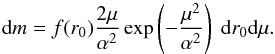 (9)As we have already
mentioned, most of the particles have r0 ~ Rvir, and
therefore only those with small μ can penetrate into the area of our interest
r ~
rcore ≪ Rvir.
This means that the distribution in the halo center is mainly determined by the behavior of
Eq. (9) at μ ≃ 0, where Eq. (9) is finite. Thus our calculation is not
sensitive to the distribution over μ: we would obtain a very similar result for any
other distribution, which has the same value 2μf(r0)
/α2(r0)
when μ → 0.
(9)As we have already
mentioned, most of the particles have r0 ~ Rvir, and
therefore only those with small μ can penetrate into the area of our interest
r ~
rcore ≪ Rvir.
This means that the distribution in the halo center is mainly determined by the behavior of
Eq. (9) at μ ≃ 0, where Eq. (9) is finite. Thus our calculation is not
sensitive to the distribution over μ: we would obtain a very similar result for any
other distribution, which has the same value 2μf(r0)
/α2(r0)
when μ → 0.
Since the particle energy conserves 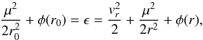 (10)the radial and
tangential components of the particle velocity are equal to
(10)the radial and
tangential components of the particle velocity are equal to 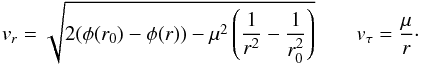 (11)The zero of the radicand
gives us the maximum angular momentum of a particle with which it can reach radius
r,
(11)The zero of the radicand
gives us the maximum angular momentum of a particle with which it can reach radius
r,
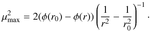 (12)We may rewrite Eq. (11) as
 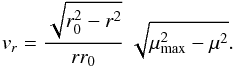 (13)We also need the
half-period of the particle, that is, the time it takes for the particle to fall from its
largest to the smallest radius,
(13)We also need the
half-period of the particle, that is, the time it takes for the particle to fall from its
largest to the smallest radius, 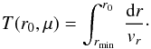 (14)T is, generally speaking, a
function of r0 and μ. However, as was shown in
Baushev (2014), for the particles that can reach the
cental region the dependence on μ is extremely weak (the reason is that the function
T(r0,μ)
slowly changes near the extremum at μ = 0). Therefore we may approximate T(r0,μ) ≃
T(r0,0) ≡
T(r0).
(14)T is, generally speaking, a
function of r0 and μ. However, as was shown in
Baushev (2014), for the particles that can reach the
cental region the dependence on μ is extremely weak (the reason is that the function
T(r0,μ)
slowly changes near the extremum at μ = 0). Therefore we may approximate T(r0,μ) ≃
T(r0,0) ≡
T(r0).
A particle of mass m contributes to the halo density throughout the
interval between r0 and the smallest radius the particle can
reach. The contribution in an interval dr is proportional to the time the particle spends in
this interval (Baushev 2011) 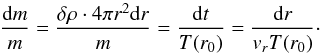 (15)Here
δρ is the
contribution of the particle to the total halo density at radius r. We obtain that
(15)Here
δρ is the
contribution of the particle to the total halo density at radius r. We obtain that
 .
To determine the total halo density, we substitute here a mass element (9) instead of m and integrate over
dr0 and dμ,
.
To determine the total halo density, we substitute here a mass element (9) instead of m and integrate over
dr0 and dμ, 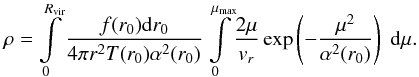 (16)If we substitute Eq. (13) for vr, the second integral can
be taken analytically:
(16)If we substitute Eq. (13) for vr, the second integral can
be taken analytically: 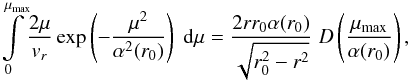 (17)where
 is the Dawson function. Since we
calculate the density profile of the central region and use assumption r ≪
r0, we can significantly simplify Eq. (17). In particular, it follows from Eq. (12) that
is the Dawson function. Since we
calculate the density profile of the central region and use assumption r ≪
r0, we can significantly simplify Eq. (17). In particular, it follows from Eq. (12) that 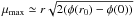 .
We obtain
.
We obtain 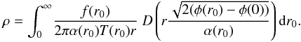 (18)We can factor out the
Dawson function from the integral using the above-mentioned properties of function
f(r0) (see the end of the
Energy distribution section). First, it is almost equal to zero for small r0: this means
that the integration in Eq. (18) is
performed not from 0, but from
.
Second, as we could see, the formed halo is dominated by the particles with r0 ~
Rvir. It follows that the main contribution
to the integral in Eq. (18) is given by the
part close to the upper limit r0 ≃ Rvir:
roughly speaking, by r0 ∈ [ Rvir/
2;Rvir ]. These two properties of
f(r0) mean that
f(r0) sharply depends on
r0
at this interval. Conversely, α(r0) probably does not
change much in interval [
Rvir/ 2;Rvir
]: α(r0) is widely believed
to be a power-law dependence with the index between −1 and 1 (Hansen et
al. 2006).
(18)We can factor out the
Dawson function from the integral using the above-mentioned properties of function
f(r0) (see the end of the
Energy distribution section). First, it is almost equal to zero for small r0: this means
that the integration in Eq. (18) is
performed not from 0, but from
.
Second, as we could see, the formed halo is dominated by the particles with r0 ~
Rvir. It follows that the main contribution
to the integral in Eq. (18) is given by the
part close to the upper limit r0 ≃ Rvir:
roughly speaking, by r0 ∈ [ Rvir/
2;Rvir ]. These two properties of
f(r0) mean that
f(r0) sharply depends on
r0
at this interval. Conversely, α(r0) probably does not
change much in interval [
Rvir/ 2;Rvir
]: α(r0) is widely believed
to be a power-law dependence with the index between −1 and 1 (Hansen et
al. 2006).  changes even more slowly: for instance,
  for the NFW profile with
cvir =
15. Moreover, D is a finite and not very sharp function of its
argument. Comparing this with the sharp behavior of f(r0), we may neglect the
weak dependence of the argument of function D in Eq. (18) on r0 and substitute some value, averaged over
the halo (see the Appendix for details),
for the NFW profile with
cvir =
15. Moreover, D is a finite and not very sharp function of its
argument. Comparing this with the sharp behavior of f(r0), we may neglect the
weak dependence of the argument of function D in Eq. (18) on r0 and substitute some value, averaged over
the halo (see the Appendix for details), 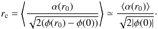 (19)Then we can rewrite Eq.
(18) and obtain the final result:
(19)Then we can rewrite Eq.
(18) and obtain the final result:
 (20)Since
D(r/rc)
≃ r/rc,
when r/rc →
0, ρc is really the central density of the
halo. As we can see, it is always finite. At the same time, the shape of the density profile
only depends on parameter rc.
(20)Since
D(r/rc)
≃ r/rc,
when r/rc →
0, ρc is really the central density of the
halo. As we can see, it is always finite. At the same time, the shape of the density profile
only depends on parameter rc.
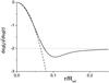 |
Fig. 2 Density profile of the model under consideration (20) (with rc = 0.05Rvir, solid line). An Einasto profile with n = 0.5 and rs = 0.017Rvir is plotted for comparison (dashed line). |
4. Discussion
Figure 2 represents profile (20) with rc = 0.05Rvir (solid line). An Einasto profile with n = 0.5 and rs = 0.017Rvir is plotted for comparison (dashed line). The model profile is very similar to the Einasto profile in the center; consequently, it fits experimental data well (Chemin et al. 2011). The second consequence is that Eq. (20) describes a cored profile with rcore ≃ rc; using criterion (1), we obtain rcore ≃ 0.924rc.
Profile (20) in all conditions transforms
into ρ ∝
r-2 at large distances, which may explain
the persistence of the flat regions in the rotation curves of a vast collection of galaxies
with very different physical properties. However, a question arises: we assume that
r0 ≫
r during the derivation of Eq. (20). Is this approximation (and, consequently,
Eq. (20)) still valid for large
r, where the
profile behaves as ρ ∝
r-2? As we showed, Eq. (20) is valid for
 .
Meanwhile, the ρ ∝
r-2 profile appears if r ≫
rc. The value of rc depends on
⟨ α ⟩ and
.
Meanwhile, the ρ ∝
r-2 profile appears if r ≫
rc. The value of rc depends on
⟨ α ⟩ and
 according to Eq. (19). We show below that
the best agreement between the theory and observations is achieved if ⟨ α ⟩ is respectively small
(32). Substituting Eq. (32) and | φ(0) | ≃
cvirΦ into (19), we can roughly estimate
according to Eq. (19). We show below that
the best agreement between the theory and observations is achieved if ⟨ α ⟩ is respectively small
(32). Substituting Eq. (32) and | φ(0) | ≃
cvirΦ into (19), we can roughly estimate 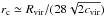 . We
illustrate this on the example of the Milky Way galaxy. Here
kpc, that is, approximately the
disk radius;
. We
illustrate this on the example of the Milky Way galaxy. Here
kpc, that is, approximately the
disk radius;  kpc,
which is comparable with the bulge size. So
kpc,
which is comparable with the bulge size. So  , Eq. (20) is still valid for r ≫
rc, and we may expect an extended region with
ρ ∝
r-2 between ~2rc ≃ 3.2 and ~30 kpc.
, Eq. (20) is still valid for r ≫
rc, and we may expect an extended region with
ρ ∝
r-2 between ~2rc ≃ 3.2 and ~30 kpc.
Now we can investigate how the multiplication ρcrc depends
on the halo mass in our model. According to Eq. (20),  (21)We can
significantly simplify this equation with the help of the same technic that we used to
transform Eqs. (18) into (20) (see Appendix): neglect the fairly weak
dependencies of functions α(r0) and T(r0) on r0 (compared with
f(r0)), and substitute
some values, averaged over the halo. Then Eq. (20) may be rewritten as
(21)We can
significantly simplify this equation with the help of the same technic that we used to
transform Eqs. (18) into (20) (see Appendix): neglect the fairly weak
dependencies of functions α(r0) and T(r0) on r0 (compared with
f(r0)), and substitute
some values, averaged over the halo. Then Eq. (20) may be rewritten as  (22)Now we estimate
⟨ α ⟩ and
⟨ T ⟩. To
begin with, we assume that ⟨ α
⟩ has the highest possible value: it can hardly be higher than
(22)Now we estimate
⟨ α ⟩ and
⟨ T ⟩. To
begin with, we assume that ⟨ α
⟩ has the highest possible value: it can hardly be higher than
 (23)because
a significant fraction of the halo particles would not be gravitationally bound in the
opposite case. Below we discuss the applicability of this assumption.
(23)because
a significant fraction of the halo particles would not be gravitationally bound in the
opposite case. Below we discuss the applicability of this assumption.
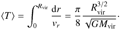
The half-period T(r0) is mainly
determined by the gravitational acceleration at r0 (where vr =
0) and is not very sensitive to the density distribution in the halo
center. As we showed, a significant part of the particles should have r0 ~
Rvir. Therefore we accept as an estimate of
⟨ T ⟩ the
time necessary for a particle with no angular momentum to fall from r =
Rvir/ 2 on a point mass,
 (24)Indeed, ⟨ r0 ⟩ can hardly
be smaller than Rvir/ 2: as we showed,
r0 ~
Rvir for most of the particles in our
model. On the other hand, we underestimate ⟨
T ⟩ by considering a point mass instead of the real
distribution. Consequently, Eq. (24) most
likely underestimates ⟨ T
⟩.
(24)Indeed, ⟨ r0 ⟩ can hardly
be smaller than Rvir/ 2: as we showed,
r0 ~
Rvir for most of the particles in our
model. On the other hand, we underestimate ⟨
T ⟩ by considering a point mass instead of the real
distribution. Consequently, Eq. (24) most
likely underestimates ⟨ T
⟩.
It is convenient to introduce ϱ – the average halo density:
 . Substituting Eqs. (23) and (24) to (22), we obtain
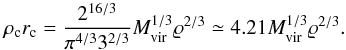 (25)As Mvir grows,
multiplier
(25)As Mvir grows,
multiplier  slowly increases, while ϱ2
/ 3 slowly decreases, since smaller halos
formed at higher z, when the Universe density was higher. Roughly
speaking, the density of a structure is proportional to the density of the Universe at the
moment z when
it collapsed (Cooray & Sheth 2002), that is,
ϱ ∝ (z +
1)3. Indeed, structures form when their density contrast
δρ/ρ reaches a
certain value (close to 1) that
does not depend on the mass (Gorbunov & Rubakov
2010, Sect. 7.2.2). Strictly speaking, the dependence of z on Mvir is ambiguous:
the initial perturbations can be considered as a random Gaussian field, and structures of
the same mass can collapse at different z. Nevertheless, we may consider an averaged redshift
z of the
collapse of structures of mass Mvir.
slowly increases, while ϱ2
/ 3 slowly decreases, since smaller halos
formed at higher z, when the Universe density was higher. Roughly
speaking, the density of a structure is proportional to the density of the Universe at the
moment z when
it collapsed (Cooray & Sheth 2002), that is,
ϱ ∝ (z +
1)3. Indeed, structures form when their density contrast
δρ/ρ reaches a
certain value (close to 1) that
does not depend on the mass (Gorbunov & Rubakov
2010, Sect. 7.2.2). Strictly speaking, the dependence of z on Mvir is ambiguous:
the initial perturbations can be considered as a random Gaussian field, and structures of
the same mass can collapse at different z. Nevertheless, we may consider an averaged redshift
z of the
collapse of structures of mass Mvir.
We have accepted for the Milky Way Mvir = MMW = 1012 M⊙, Rvir = 250 kpc (Klypin et al. 2002). It corresponds to ϱMW = 1.5·104 M⊙ kpc-3. Instead of Mvir, we can characterize the structures by the present-day wave number k of the primordial perturbations from which they were formed. Of course, Mvir ∝ k-3. The Milky Way mass Mvir ≃ 1012 M⊙ corresponds to kMW ≃ (0.6 Mpc)-1 (Gorbunov & Rubakov 2010). So k = kMW(Mvir/MMW)−1 / 3.
The shape of dependence z(Mvir) is defined by the
cosmological model. We consider the very standard ΛCDM scenario with H0 = 67.3 (Mpc-1 km s-1) (i.e.,
 s), Ωm = 0.315 (Planck Collaboration XVI 2014). In this case, z logarithmically depends on
Mvir (Gorbunov & Rubakov 2010, Eq. (5.47))
s), Ωm = 0.315 (Planck Collaboration XVI 2014). In this case, z logarithmically depends on
Mvir (Gorbunov & Rubakov 2010, Eq. (5.47)) 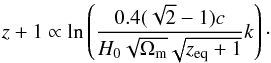 (26)We accept zeq = 3100 for the
equi-density redshift of radiation and matter (Gorbunov
& Rubakov 2010). Substituting here ϱ ∝ (z +
1)3 and k =
kMW(Mvir/MMW)−1 / 3, we obtain
(26)We accept zeq = 3100 for the
equi-density redshift of radiation and matter (Gorbunov
& Rubakov 2010). Substituting here ϱ ∝ (z +
1)3 and k =
kMW(Mvir/MMW)−1 / 3, we obtain ![\begin{equation} \label{16a22} \varrho\propto \ln^3\left[\dfrac{0.4(\sqrt2-1) c k_{\rm MW}}{H_0 \sqrt{\Omega_{\rm m}} \sqrt{z_{\rm eq}+1}} \left(\dfrac{\mvir}{M_{\rm MW}}\right)^{-1/3}\right]\cdot \end{equation}](/articles/aa/full_html/2014/09/aa22730-13/aa22730-13-eq216.png) (27)It is convenient to
introduce
(27)It is convenient to
introduce 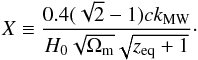 (28)Then Eq. (27) may be rewritten as
 ![\begin{equation} \label{16a24} \varrho\propto \ln^3\left[X \left(\mvir/M_{\rm MW}\right)^{-1/3}\right] \propto\left(1-\dfrac{\ln\left(\mvir/M_{\rm MW}\right)}{3\ln X} \right)^3\cdot \end{equation}](/articles/aa/full_html/2014/09/aa22730-13/aa22730-13-eq218.png) (29)Consequently,
(29)Consequently,
 (30)Now we can insert
this value into Eq. (25). To compare the
result with observations, we need to calculate ρcrb instead
of ρcrc. By using
a profile-independent definition of the core radius (1), we obtain rcore = rb/
2 and rcore ≃
0.924rc. Consequently, ρcrc ≃
0.541ρcrb, and
we derive the final result
(30)Now we can insert
this value into Eq. (25). To compare the
result with observations, we need to calculate ρcrb instead
of ρcrc. By using
a profile-independent definition of the core radius (1), we obtain rcore = rb/
2 and rcore ≃
0.924rc. Consequently, ρcrc ≃
0.541ρcrb, and
we derive the final result  (31)Observations
suggest that log (ρcrb) ≃ const. = 2.15 ±
0.2 in units of log (M⊙ pc-2) for a large array
of elliptic and spiral galaxies, and probably for the Local Group dwarf spheroidal galaxies
(Donato et al. 2009). Figure 3 represents the dependence (25) (solid line) predicted by the moderate relaxation model. Clearly, the
multiplication ρcrb is not
perfectly constant; however, it changes only by a factor of three when the virial mass of
galaxies varies from 109 M⊙ to 1012 M⊙,
which covers almost the entire galaxy mass range. This means that the variation of
ρcrb does not
exceed the 3σ
interval of the observations, and from this point of view, ρcrb may be
considered as constant.
(31)Observations
suggest that log (ρcrb) ≃ const. = 2.15 ±
0.2 in units of log (M⊙ pc-2) for a large array
of elliptic and spiral galaxies, and probably for the Local Group dwarf spheroidal galaxies
(Donato et al. 2009). Figure 3 represents the dependence (25) (solid line) predicted by the moderate relaxation model. Clearly, the
multiplication ρcrb is not
perfectly constant; however, it changes only by a factor of three when the virial mass of
galaxies varies from 109 M⊙ to 1012 M⊙,
which covers almost the entire galaxy mass range. This means that the variation of
ρcrb does not
exceed the 3σ
interval of the observations, and from this point of view, ρcrb may be
considered as constant.
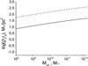 |
Fig. 3 Value (31) of ρcrb for various halo masses (solid line). For the entire range of galactic masses (Mvir ≃ 109−1012 M⊙) multiplication ρcrb remains almost constant. According to Eq. (22), ρcrb is inversely proportional to ⟨ α ⟩. The dashed line represents ρcrb, if we use a lower value of ⟨ α ⟩ (Eq. (32) instead of (23)). This agrees well with observations (log (ρcrb) = 2.15 ± 0.2 in units of log (M⊙ pc-2)). |
Thus, the moderate evolution model naturally predicts an almost constant multiplication
ρcrb in the
galaxy mass range, which agrees well with observations. On the other hand, the value of the
constant ρcrb predicted
by Eq. (25) is lower approximately by a
factor of seven than the observed value. The contradiction may be obviated if we assume that
supposition (23) of the value of
⟨ α ⟩ is not
true. Indeed, Eq. (23) implies that
⟨ α ⟩ has the
highest possible value. This is not necessarily so; moreover, there are some reasons to
believe that the mean-square-root angular momentum of the particles of DM halos is fairly
small (Baushev 2011). According to Eq. (22), ρcrb is
inversely proportional to ⟨ α
⟩. If we insert  (32)instead
of Eq. (23) into (22), we obtain the dependence of ρcrb on
Mvir in excellent agreement with
observations (the dashed line in Fig. 3).
(32)instead
of Eq. (23) into (22), we obtain the dependence of ρcrb on
Mvir in excellent agreement with
observations (the dashed line in Fig. 3).
It is important to underline that concluding about the constancy of the multiplication
ρcrb for the
galaxy mass objects is an inherent property of the moderate-relaxation model and does not
depend on the choice of constants in Eqs. (23) and (32). For more massive
halos (Mvir ≥
1013 M⊙) the model predicts an
even weaker dependence of ρcrb on
Mvir; however, the model itself is hardly
adequate for objects this massive. Very small halos (Mvir<
106 M⊙) should have
 , that
is, ρcrb is not
quite constant anymore. However, the dependence remains rather weak.
, that
is, ρcrb is not
quite constant anymore. However, the dependence remains rather weak.
5. Conclusion
Thus assuming moderate relaxation in the formation of dark matter halos invariably leads to density profiles that match those observed in the central regions of galaxies. The profile is insensitive to the initial conditions. It has a central core; in the core area the density distribution behaves as an Einasto profile with a low index (n ~ 0.5). At larger distances it has an extended region with ρ ∝ r-2. The multiplication of the central density by the core radius is almost independent of the halo mass.
This is exactly the shape that observations suggest for the central region of galaxies. On the other hand, it does not fit the galaxy cluster profiles. This implies that the relaxation of huge objects (Mvir> 1013 M⊙, galaxy clusters) is violent. However, it is moderate for galaxies or smaller objects.
The most plausible explanation of this fact is that the concentrations cvir of small halos are much higher. As we showed, for the relaxation to be violent, the energies of a significant part of the particles need to change by a factor ~cvir with respect to the initial values (so that these particles have r0 ≃ 0 and form the cusp). Consequently, for galaxy clusters the relaxation is violent if the energies of the particles decrease by a factor 3–5 (cvir = 3−5 for these objects). Such a change seems possible even in a collisionless system. However, cvir ~ 15 even for massive galaxies and can be much higher for dwarf objects. Then the violent relaxation claims that the energies of a significant fraction of the particles change by a factor 15–20: this requirement is quite strong. Probably, some other factors, such as the baryon component, also influence the intensity of the relaxation. This question merits a more detailed consideration.
Acknowledgments
Financial support by Bundesministerium für Bildung und Forschung through DESY-PT, grant 05A11IPA, is gratefully acknowledged. BMBF assumes no responsibility for the contents of this publication. We acknowledge support by the Helmholtz Alliance for Astroparticle Physics HAP funded by the Initiative and Networking Fund of the Helmholtz Association.
References
- Baushev, A. N. 2011, MNRAS, 417, L83 [NASA ADS] [CrossRef] [Google Scholar]
- Baushev, A. N. 2012, MNRAS, 420, 590 [NASA ADS] [CrossRef] [Google Scholar]
- Baushev, A. N. 2013a, ApJ, 771, 117 [NASA ADS] [CrossRef] [Google Scholar]
- Baushev, A. N. 2013b, Astropart. Phys., accepted [arXiv:1312.0314] [Google Scholar]
- Baushev, A. N. 2014, ApJ, 786, 65 [NASA ADS] [CrossRef] [Google Scholar]
- Binney, J., & Tremaine, S. 2008, Galactic Dynamics: 2d edn. (Princeton University Press) [Google Scholar]
- Burkert, A. 1995, ApJ, 447, L25 [NASA ADS] [CrossRef] [Google Scholar]
- Carney, B. W., & Latham, D. W. 1987, in Dark matter in the Universe, eds. J. Kormendy, & G. R. Knapp, IAU Symp., 117, 39 [Google Scholar]
- Chemin, L., de Blok, W. J. G., & Mamon, G. A. 2011, AJ, 142, 109 [NASA ADS] [CrossRef] [Google Scholar]
- Cooray, A., & Sheth, R. 2002, Phys. Rep., 372, 1 [NASA ADS] [CrossRef] [Google Scholar]
- de Blok, W. J. G., & Bosma, A. 2002, A&A, 385, 816 [NASA ADS] [CrossRef] [EDP Sciences] [Google Scholar]
- de Blok, W. J. G., McGaugh, S. S., & Rubin, V. C. 2001, AJ, 122, 2396 [NASA ADS] [CrossRef] [Google Scholar]
- Diemand, J., & Kuhlen, M. 2008, ApJ, 680, L25 [NASA ADS] [CrossRef] [Google Scholar]
- Diemand, J., Madau, P., & Moore, B. 2005, MNRAS, 364, 367 [NASA ADS] [CrossRef] [Google Scholar]
- Diemand, J., Kuhlen, M., & Madau, P. 2007, ApJ, 667, 859 [NASA ADS] [CrossRef] [Google Scholar]
- Donato, F., Gentile, G., Salucci, P., et al. 2009, MNRAS, 397, 1169 [NASA ADS] [CrossRef] [Google Scholar]
- Evans, N. W., & Collett, J. L. 1997, ApJ, 480, L103 [NASA ADS] [CrossRef] [Google Scholar]
- Gentile, G., Salucci, P., Klein, U., & Granato, G. L. 2007, MNRAS, 375, 199 [NASA ADS] [CrossRef] [Google Scholar]
- Gorbunov, D. S. & Rubakov, V. A. 2010, Introduction to the Early Universe theory. Vol. 2: Cosmological perturbations. (Moscow: LKI publishing house) [Google Scholar]
- Governato, F., Zolotov, A., Pontzen, A., et al. 2012, MNRAS, 422, 1231 [NASA ADS] [CrossRef] [Google Scholar]
- Hansen, S. H., Moore, B., Zemp, M., & Stadel, J. 2006, J. Cosmol. Astropart, 1, 14 [Google Scholar]
- Hayashi, E., Navarro, J. F., Taylor, J. E., Stadel, J., & Quinn, T. 2003, ApJ, 584, 541 [NASA ADS] [CrossRef] [Google Scholar]
- Klypin, A., Zhao, H., & Somerville, R. S. 2002, ApJ, 573, 597 [Google Scholar]
- Klypin, A., Prada, F., Yepes, G., Hess, S., & Gottlober, S. 2013, MNRAS, submitted [arXiv:1310.3740] [Google Scholar]
- Kormendy, J., & Freeman, K. C. 2004, in Dark Matter in Galaxies, eds. S. Ryder, D. Pisano, M. Walker, & K. Freeman, IAU Symp., 220, 377 [Google Scholar]
- Kuhlen, M., Weiner, N., Diemand, J., et al. 2010, J. Cosmology Astropart. Phys., 2, 30 [NASA ADS] [CrossRef] [Google Scholar]
- Landau, L. D., & Lifshitz, E. M. 1980, Statistical physics, Pt.1, Pt.2 (Oxford: Pergamon Press) [Google Scholar]
- Lynden-Bell, D. 1967, MNRAS, 136, 101 [NASA ADS] [CrossRef] [Google Scholar]
- Marchesini, D., D’Onghia, E., Chincarini, G., et al. 2002, ApJ, 575, 801 [NASA ADS] [CrossRef] [Google Scholar]
- Marochnik, L. S., & Suchkov, A. A. 1984, The Galaxy (Moscow: izdatel’stvo Nauka) [in Russian] [Google Scholar]
- Moore, B., Quinn, T., Governato, F., Stadel, J., & Lake, G. 1999, MNRAS, 310, 1147 [NASA ADS] [CrossRef] [Google Scholar]
- Navarro, J. F., Ludlow, A., Springel, V., et al. 2010, MNRAS, 402, 21 [NASA ADS] [CrossRef] [Google Scholar]
- Neto, A. F., Gao, L., Bett, P., et al. 2007, MNRAS, 381, 1450 [NASA ADS] [CrossRef] [Google Scholar]
- Oh, S.-H., de Blok, W. J. G., Brinks, E., Walter, F., & Kennicutt, Jr., R. C. 2011, AJ, 141, 193 [NASA ADS] [CrossRef] [Google Scholar]
- Okabe, N., Zhang, Y.-Y., Finoguenov, A., et al. 2010, ApJ, 721, 875 [NASA ADS] [CrossRef] [Google Scholar]
- Planck Collaboration XVI. 2014, A&A, in press DOI: 10.1051/0004-6361/201321591 [Google Scholar]
- Power, C., Navarro, J. F., Jenkins, A., et al. 2003, MNRAS, 338, 14 [NASA ADS] [CrossRef] [Google Scholar]
- Quinlan, G. D. 1996, New A, 1, 255 [Google Scholar]
- Rubin, V. C., Thonnard, N., & Ford, Jr., W. K. 1978, ApJ, 225, L107 [NASA ADS] [CrossRef] [Google Scholar]
- Salucci, P., Lapi, A., Tonini, C., et al. 2007, MNRAS, 378, 41 [NASA ADS] [CrossRef] [Google Scholar]
- Sofue, Y., & Rubin, V. 2001, ARA&A, 39, 137 [NASA ADS] [CrossRef] [Google Scholar]
- Stadel, J., Potter, D., Moore, B., et al. 2009, MNRAS, 398, L21 [NASA ADS] [CrossRef] [Google Scholar]
- Tollerud, E. J., Beaton, R. L., Geha, M. C., et al. 2012, ApJ, 752, 45 [NASA ADS] [CrossRef] [Google Scholar]
- Wang, J., Frenk, C. S., Navarro, J. F., Gao, L., & Sawala, T. 2012, MNRAS, 424, 2715 [NASA ADS] [CrossRef] [Google Scholar]
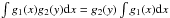
Appendix A: A convolution of two functions: how does one transform Eq. (18) into (20)?
We consider a convolution of two functions  where g1(x) is finite, that is,
g1(x) differs
noticeably from zero only in a narrow interval x ∈ [
x1,x2
], and g2(x,y) depend only
slightly on x
at this interval for any given y. Then we may roughly estimate
where g1(x) is finite, that is,
g1(x) differs
noticeably from zero only in a narrow interval x ∈ [
x1,x2
], and g2(x,y) depend only
slightly on x
at this interval for any given y. Then we may roughly estimate 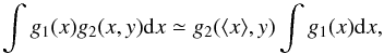 (A.1)where
⟨ x ⟩ is
the value of x averaged over [
x1,x2
]. Indeed, Eq. (A.1)
becomes exact if the width of g1(x) is negligible
∫δ(x −
x0)g2(x,y)dx
=
g2(x0,y).
It is also exact if g2(x,y) does not change
at all, when x runs between x1 and
x2:
(A.1)where
⟨ x ⟩ is
the value of x averaged over [
x1,x2
]. Indeed, Eq. (A.1)
becomes exact if the width of g1(x) is negligible
∫δ(x −
x0)g2(x,y)dx
=
g2(x0,y).
It is also exact if g2(x,y) does not change
at all, when x runs between x1 and
x2:
 . If g2(x,y) depends on
x at
[
x1,x2
], Eq. (A.1) is an
approximation. However, our prime interest here is the accuracy of transformation (18) into (20) with the help of Eq. (A.1). We show below that the approximation is quite good in this case.
. If g2(x,y) depends on
x at
[
x1,x2
], Eq. (A.1) is an
approximation. However, our prime interest here is the accuracy of transformation (18) into (20) with the help of Eq. (A.1). We show below that the approximation is quite good in this case.
First of all, we should determine the best way to find rc (see Eq.
(19)), that is, to average
 over the halo. Since we are interested in the very central region of the halo, we consider
the case when r →
0. The Dawson function D(x) ≃ x if
x is small,
and we obtain from Eq. (18)
over the halo. Since we are interested in the very central region of the halo, we consider
the case when r →
0. The Dawson function D(x) ≃ x if
x is small,
and we obtain from Eq. (18) 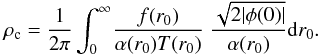 (A.2)Dividing this
equation by (21), we obtain
(A.2)Dividing this
equation by (21), we obtain 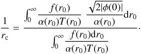 (A.3)This equation can be
considered as a sort of averaging of function
(A.3)This equation can be
considered as a sort of averaging of function  over the halo with the use of
  as the weighting function. This method of averaging yields the best fitting of Eq. (18) in the halo center.
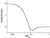 |
Fig. A.1 Shapes of density profiles calculated with the help of the exact Eq. (18) (solid line) and approximation (20) (dashed line, see the Appendix for details). |
To estimate the accuracy of transformation (18) into (20), we may consider a
more or less realistic model of functions f(r0), α(r0), T(r0), and then to
compare the density profiles obtained with the help of Eqs. (18) and (20). We
assume that f(r0) has a Gaussian
shape  (A.4)where
a =
0.7Rvir, σ =
0.2Rvir. The parameters are chosen so that
the total final energy of the halo is approximately equal to the initial one,
f(r0) is finite, as
described at the end of the Energy distribution section, and the region
falls approximately outside the 3σ area, if cvir ~ 15, which
is a typical value for galaxies. T(r0) is mainly defined
by the particle motion near the apocenter (Baushev
2013a). Since M(r0) ≃
Mvir if r0 ~
Rvir, we may assume that
(A.4)where
a =
0.7Rvir, σ =
0.2Rvir. The parameters are chosen so that
the total final energy of the halo is approximately equal to the initial one,
f(r0) is finite, as
described at the end of the Energy distribution section, and the region
falls approximately outside the 3σ area, if cvir ~ 15, which
is a typical value for galaxies. T(r0) is mainly defined
by the particle motion near the apocenter (Baushev
2013a). Since M(r0) ≃
Mvir if r0 ~
Rvir, we may assume that
 ,
as in the case of a point mass Mvir. The same reasoning allows us to
assume by analogy with Eqs. (23) and
(32) that
,
as in the case of a point mass Mvir. The same reasoning allows us to
assume by analogy with Eqs. (23) and
(32) that
 ,
and that
,
and that  .
A normalization of f(r0), α(r0), and
T(r0) is not
significant, since we are interested in the profile shape, and we plot it in
log ρ/
log r coordinates. However, we choose a proper value
of
to obtain a desirable value of rc according to Eq. (A.3). We chose rc =
0.05Rvir, exactly as in Fig. 2.
.
A normalization of f(r0), α(r0), and
T(r0) is not
significant, since we are interested in the profile shape, and we plot it in
log ρ/
log r coordinates. However, we choose a proper value
of
to obtain a desirable value of rc according to Eq. (A.3). We chose rc =
0.05Rvir, exactly as in Fig. 2.
Figure A.1 represents the density profiles calculated for this model with the help of exact Eq. (18) (solid line) and approximation (20) (dashed line). Clearly, the deviations are quite small, especially in the halo center and at large radii. Moreover, approximation (20) has the same shape as the exact solution,
that is, the same Einasto-like profile in the center, the same core radius, and the same ρ ∝ r-2 region. Consequently, the conclusions of this paper are valid for the exact solution (18) as well. Thus the approximation of Eq. (18) by (20) is quite accurate for realistic models of halo parameters.
All Figures
|
Fig. 1 Initial energy spectra |
| In the text | |
|
Fig. 2 Density profile of the model under consideration (20) (with rc = 0.05Rvir, solid line). An Einasto profile with n = 0.5 and rs = 0.017Rvir is plotted for comparison (dashed line). |
| In the text | |
|
Fig. 3 Value (31) of ρcrb for various halo masses (solid line). For the entire range of galactic masses (Mvir ≃ 109−1012 M⊙) multiplication ρcrb remains almost constant. According to Eq. (22), ρcrb is inversely proportional to ⟨ α ⟩. The dashed line represents ρcrb, if we use a lower value of ⟨ α ⟩ (Eq. (32) instead of (23)). This agrees well with observations (log (ρcrb) = 2.15 ± 0.2 in units of log (M⊙ pc-2)). |
| In the text | |
|
Fig. A.1 Shapes of density profiles calculated with the help of the exact Eq. (18) (solid line) and approximation (20) (dashed line, see the Appendix for details). |
| In the text | |
Current usage metrics show cumulative count of Article Views (full-text article views including HTML views, PDF and ePub downloads, according to the available data) and Abstracts Views on Vision4Press platform.
Data correspond to usage on the plateform after 2015. The current usage metrics is available 48-96 hours after online publication and is updated daily on week days.
Initial download of the metrics may take a while.