| Issue |
A&A
Volume 569, September 2014
|
|
|---|---|---|
| Article Number | A2 | |
| Number of page(s) | 17 | |
| Section | Astronomical instrumentation | |
| DOI | https://doi.org/10.1051/0004-6361/201220223 | |
| Published online | 08 September 2014 | |
Comparison of fringe-tracking algorithms for single-mode near-infrared long-baseline interferometers
1 LESIA, Observatoire de Paris, CNRS, UPMC, Université Paris-Diderot, Paris Sciences et Lettres Research University, 5 place Jules Janssen, 92 195 Meudon, France
e-mail: This email address is being protected from spambots. You need JavaScript enabled to view it.
2 Groupement d’Intérêt Scientifique PHASE (Partenariat Haute résolution Angulaire Sol Espace) between ONERA, Observatoire de Paris, CNRS and Université Paris Diderot
3 Space Telescope Science Institute, 3700 San Martin Drive, Baltimore MD 21218, USA
4 Instituut voor Sterrenkunde, KU Leuven, Celestijnenlaan 200D, 3001 Leuven, Belgium
5 Onera – The French Aerospace Lab, BP 72, 92 322 Châtillon, France
6 Max Planck Institute for extraterrestrial Physics, PO Box 1312, Giessenbachstr., 85 741 Garching, Germany
Received: 14 August 2012
Accepted: 17 June 2014
Abstract
To enable optical long baseline interferometry toward faint objects, long integrations are necessary despite atmospheric turbulence. Fringe trackers are needed to stabilize the fringes and thus increase the fringe visibility and phase signal-to-noise ratio (S/N), with efficient controllers robust to instrumental vibrations and to subsequent path fluctuations and flux drop-outs. We report on simulations, analysis, and comparison of the performances of a classical integrator controller and of a Kalman controller, both optimized to track fringes under realistic observing conditions for different source magnitudes, disturbance conditions, and sampling frequencies. The key parameters of our simulations (instrument photometric performance, detection noise, turbulence, and vibrations statistics) are based on typical observing conditions at the Very Large Telescope observatory and on the design of the GRAVITY instrument, a 4-telescope single-mode long-baseline interferometer in the near-infrared, next in line to be installed at VLT Interferometer. We find that both controller performances follow a two-regime law with the star magnitude, a constant disturbance limited regime, and a diverging regime limited by both the detector and photon-noise. Moreover, we find that the Kalman controller is optimal in the high and medium S/N regime owing to its predictive commands based on an accurate disturbance model. In the low S/N regime, the model is not accurate enough to be more robust than an integrator controller. Identifying the disturbances from high S/N measurements improves the Kalman performances in the case of strong optical path difference disturbances.
Key words: instrumentation: high angular resolution / atmospheric effects / methods: numerical / techniques: interferometric
PhD Fellow of the Research Foundation – Flanders (FWO).
© ESO, 2014
1. Introduction
Atmospheric turbulence is a major limiting factor for the sensitivity of ground-based optical long-baseline interferometers. Because of the short coherence time of atmospheric turbulence – typically τ0 = 20 ms in the near infrared – basic observations are indeed limited to short exposure times and, as a consequence, to bright targets. With long exposures, the random fringe motion induced by the turbulent atmosphere would completely blur fringe contrast and would provide poor phase and visibility measurements.
To overcome this limitation, a servo-system called fringe tracking was developed by Shao & Staelin (1977) and demonstrated three years later (Shao & Staelin 1980). By stabilizing the interferometric fringes to a fraction of the wavelength, such a system indeed enables exposure times of several minutes without the visibility loss inherent in the fringe motion, and therefore gives access to new sensitivity limits. Fringe trackers have since proven themselves to be essential, not only to observe faint targets (Müller et al. 2010; Colavita et al. 2013), but also to perform astrometry with a submilliarcsecond (mas) accuracy (Lane & Muterspaugh 2004). That explains why the main long baseline interferometers are currently being provided either with instruments that include their own fringe trackers: PRIMA (Delplancke et al. 2006; Sahlmann et al. 2009), GRAVITY (Eisenhauer et al. 2011) or with shared fringe trackers: the fringe tracker of the Keck Interferometer (Colavita et al. 2010), CHAMP for the CHARA array (Berger et al. 2008), and FINITO for the Very Large Telescope Interferometer (VLTI; Le Bouquin et al. 2008).
Another key parameter for reaching high sensitivity limits with an interferometer is to combine telescopes with large apertures so as to obtain a large collecting surface. However, most of the 10 m class telescopes suffer from strong vibrations, owing to their lightened structure being more subject to having vibrating frequencies excited either by the wind, by telescope movement while tracking a star, or by the instruments fixed at their different focuses, which are usually equipped with highly vibrating systems (electronics, coolers, etc.). Stabilizing fringes in these conditions are particularly challenging because vibrations lead to important path length fluctuations that add up to the atmospheric turbulence, and also generate tip-tilt variations of the beams, resulting in fluctuations of the combined flux. A classical controller is typically unable to correct for system variations because of its continuous transfer function with limited bandwidth. At best, a classical controller can dampen the lowest frequency components that are well within its bandwidth, but it cannot completely filter out disturbances at a specific frequency.
To overcome this problem, several approaches can be combined. First of all, the sources of the vibration excitations can sometimes be identified and switched off. An efficient example of these efforts have been demonstrated at VLTI these past years, bringing the optical path length variations on the 8.2 m unit telescopes (UTs) from typical values of 280 nm rms to more than 1 μm rms in 2008 down to 145 to 380 nm rms in 2012, by damping pumps of some instruments, changing the close cyclo coolers of some others, and modifying the mechanical design of some mounts (Poupar et al. 2010; Haguenauer et al. 2010, 2012). Second, vibrations excited by the first mirrors of the system can be measured with accelerometers and independently compensated by optical delay lines (Colavita et al. 2013; Haguenauer et al. 2012). However, these solutions are not enough to completely suppress vibrations down the entire optical stream, and active compensation is necessary at the beam combination level. If a handful of vibrations are properly identified and characterized by a phase sensor, individual narrow-band suppression control blocks can be used to filter them out. Such a solution was implemented at the Keck interferometer with higher harmonic controllers (HHC; Colavita et al. 2010) and at the VLTI with an adaptive version, the vibration-tracking algorithm (VTK; Di Lieto et al. 2008).
An alternative approach is to compensate all vibrations in the optical path and the atmospheric turbulence at the same time. This can be achieved with a Kalman controller, which is a predictive algorithm whose commands are based on a model of the identified disturbance components. The formalism was first developed by Kalman (1960), then was transposed to adaptive optics (AO) systems by Le Roux et al. (2004) and Petit et al. (2004). The first on-sky demonstration of full wavefront control with a Kalman filter was achieved in 2012 and 2013 on the CANARY MOAO pathfinder (Sivo et al. 2013), and Kalman-based tip-tilt correction was implemented in two extreme AO systems: the Gemini Planet Imager (GPI) at Gemini south (Hartung et al. 2013) and the Spectro-Polarimetric High-contrast Exoplanet Research (SPHERE) instrument at VLT (Petit et al. 2012). First light of these two instruments is planned in 2014. Based on these developments in wavefront control, Kalman filtering was adapted to two-way fringe tracking by Lozi et al. (2011) and to four-way fringe tracking by Menu et al. (2012).
In this paper, we aim at comparing the performances of a Kalman controller and a classical controller, both optimized to track fringes in different disturbance conditions with multiple baselines. We performed numerical simulations to analyze their robustness against several levels of instrumental vibrations and to coherent flux variations. To do so, we based our simulations on the design of the GRAVITY instrument, which is the next instrument in line to be installed at VLTI, and it therefore provides the perfect framework for comparing control algorithms for fringe tracking.
Currently, the VLTI is the most powerful observatory for matching high sensitivity and high angular resolution. On the one hand, it is indeed the only long-baseline interferometer that allows the combination of four 8.2 m UTs, hence the greatest available collecting surface to date, on 47 m to 130 m baselines, and on the other hand, it has the capacity to combine four relocatable 1.8 m auxiliary telescopes (ATs) on baselines with lengths ranging from 8 m to 202 m (only 11 m to 140 m baselines are offered at present), with a potential resolution of 2 mas at 2 μm. However, each UT is equipped with several instruments fixed at its different Cassegrain focuses that excite vibration frequencies differing from one UT to another. Despite strong efforts to minimize them, these vibrations still limit operations at VLTI (Mérand et al. 2012).
GRAVITY (General Relativity Analysis via VLT InTerferometrY) is a second-generation instrument for the VLTI that will combine up to four telescopes in the K band and is currently in phase D with first on-sky tests in 2015 (Eisenhauer et al. 2011). Its goal is to provide dual-field precision astrometry on the order of 10 μas and phase-referenced imaging with 4 mas resolution, with as primary science case the study of the close environment of Sgr A*, the supermassive black hole in the center of the Galaxy. With this objective, it will lead to unprecedented imaging of targets of magnitudes up to K = 16 with 100 s exposure time (Gillessen et al. 2010), thanks to fringe tracking on an unresolved reference star of a magnitude up to 10, which is the current best sensitivity limit in this band (Keck Interferometer, Ragland et al. 2010). To reach this goal, the fringe tracker will have to stabilize the optical path differences (OPDs) down to 350 nm rms on six interferometric baselines with the UTs under median atmospheric conditions, using a controller robust to longitudinal vibrations and coherent flux variations.
We present in this paper realistic numerical simulations of fringe tracking under different disturbance conditions based on the design of GRAVITY and compare the performances of a Kalman controller and of an integrator controller in this framework. In Sect. 2, we describe the simulation of the disturbances and in Sect. 3 the parameters used to simulate the combining and detection optical systems. In Sect. 4 we present the algorithms used to estimate the OPD on each baseline, and we explain both controllers. In Sect. 5, we describe the results of the simulations and compare the performances of the integrator and Kalman controllers for different observing conditions and reference star magnitudes. These results are discussed in Sect. 6, and comments are pointed out for the specific case of GRAVITY. Finally, the conclusions of this paper are summarized in Sect. 7.
2. Simulation of the disturbances
We analyzed the closed-loop behavior of the fringe tracker with an iterative time-domain simulator1 that reproduces the entire acquisition and control process of the fringe tracker. Discrete sequences of disturbance were generated as input for the simulator. At each iteration, the image on the fringe-tracker detector was computed from the OPD residuals and then processed by the algorithm of the fringe tracker to deduce new piston commands.
The parameters that we used to simulate the disturbances and the beam combination are based on the median atmospheric conditions at the VLT observatory at Cerro Paranal, Chile, and on the design of the fringe tracker of the GRAVITY instrument. These parameters are listed in Table 1. Moreover, we simulated different observing conditions to evaluate the robustness of the controllers. The parameters and their range of variations are listed in Table 2. Table 3 indicates the specifications of the fringe tracker of GRAVITY. We describe in this section the models used to simulate the disturbances in the system: the atmospheric piston, longitudinal vibrations, and flux variations.
Fix parameters used in the simulations.
Varying parameters and their range of variation.
Specifications of the fringe tracker of GRAVITY.
2.1. Modeling piston disturbances
As the first input of our simulator, we generate a sequence of piston fluctuations over N frames for each aperture. The sequence of piston disturbances, hereafter {Pn} n ∈ [1,N] where Pn is a four-element vector in our GRAVITY-like case, is computed from the sum of the two main causes of disturbance: the atmospheric piston and the longitudinal vibrations.
2.1.1. Atmospheric piston
To simulate the atmospheric turbulence on each aperture, we used a Von Kármán model (Reinhardt & Collins 1972) with a refractive-index spatial power spectrum ΦN proportional to  (1)with κ the spatial frequency. Unlike a basic Kolmogorov model that diverges at zero frequency, this model includes a finite atmospheric outer scale L0, which leads to the saturation of the spectrum at low frequencies and is thus more realistic.
The asymptotic OPD temporal power spectrum density (PSD) Satm for a Von Kármán model is described by Buscher et al. (1995). For given wind speed V and baseline length B, it follows an f0 law for low temporal frequencies f, an f− 2/3 power law between the two cut-off frequencies f1 ~ 0.2V/B and f2 ~ V/L0, and an f− 8/3 law for higher frequencies:  (2)Atmospheric piston sequences are simulated for each aperture by multiplying the spectrum of a white Gaussian noise sequence with this asymptotic power spectrum in Fourier space. The time sequences are then scaled to match a given atmospheric OPD standard deviation σatm when combining two apertures.
A typical value of L0 = 22 m was measured at Paranal with the Generalized Seeing Monitor (GSM) instrument in 1998 and 2007 (Martin et al. 2000; Dali Ali et al. 2010).However, we do not use this value in our simulations for two main reasons. First of all, the standard deviation predicted by Conan et al. (2000) and Maire et al. (2006) for the piston fluctuations with an atmospheric outer scale of 22 m is much lower than the typical value of 10 μm measured under median seeing conditions in the K band with PRIMA (Sahlmann et al. 2009) or in the H band with FINITO (Le Bouquin et al. 2008). The standard deviation of OPD fluctuations for different values of L0 in the K band are illustrated in Fig. 1 (top). Furthermore, at identical energy levels, the atmospheric piston spectrum with a Von Kármán model and a low outer scale value have stronger high-frequency components, which are not representative of an OPD spectrum measured at VLTI with PRIMA and FINITO (cf. Fig. 1 bottom). This important difference with the GSM measurements is attributed to an instrumental contribution from the VLTI in the OPD fluctuations (e.g., internal turbulence in the delay lines). To generate realistic disturbance sequences similar to OPD measurements at VLTI, we thus adopted a value of 100 m for the atmospheric outer scale and scaled the atmospheric disturbance to a typical standard deviation of σatm = 10 μm. In Fig. 2, we present a typical atmospheric OPD temporal sequence and PSD used for these simulations.
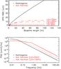 |
Fig. 1 Comparison of Kolmogorov and Von Kármán models with different atmospheric outer scale values. Top: standard deviation of OPD fluctuations as a function of the baseline length for median atmospheric conditions in the K band (Conan et al. 2000; Maire et al. 2006). Bottom: OPD temporal PSDs, scaled to have an identical energy level (standard deviation of 10 μm). |
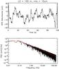 |
Fig. 2 Typical simulated atmospheric OPD disturbance, with a Von Kármán model, an atmospheric outer L0 of 100 m, and a standard deviation of 10 μm. Top: temporal sequence. Bottom: simulated PSD (black) and PSD model used for the simulation (red). |
2.1.2. Piston vibrations
To this atmospheric turbulence sequence, we add a discrete number of vibrations for each aperture to simulate the total piston disturbance sequence { Pn } n ∈ [1,N]. Strong vibrations are indeed excited by the instruments installed at the focuses of the telescopes and propagate along their mechanical structure. We modeled each narrow-band vibration peak by a damped harmonic oscillator excited by a Gaussian noise v, characterized by three parameters: the natural frequency f0, the damping coefficient k, and the variance of the excitation  . The temporal evolution pv(t) of a piston vibration is defined by the following differential equation (Petit 2006):
  (3)where T is the sampling pitch. The related temporal PSD Svib is thus expressed by
  (4)Each vibration is simulated by multiplying the model PSD with the spectrum of a white Gaussian noise sequence in the Fourier space. We assume in our simulations that the vibrations have invariant characteristics. This point is discussed further in Sect. 6.
Parameters of the vibration peaks simulated on each telescope.
Total standard deviation of vibrations per telescope, for each simulated level.
Three different levels of vibrations are tested in our simulations: no vibration at all, a low vibration level as expected in late 2014 at VLTI, and a high vibration level similar to the current level on the UTs. For the current conditions at VLTI, we used the vibration parameters listed in Table 4 for the four telescopes. These values have been chosen to reproduce similar cumulative piston vibrations and vibration spectra measured on the UTs by Di Lieto et al. (2008) and Poupar et al. (2010). The adopted damping coefficients correspond to resonance of 54 dB for the narrowest vibrations (k = 0.001) and 20 dB for the more damped ones (k = 0.05). We used the same vibration parameters for the low vibration level and scaled the total OPD standard deviations to σvib = 150 nm on each baseline. We provide a summary of the total standard deviations of the vibrations in Table 5 for the three simulated levels. In Fig. 3, we present the cumulative vibration spectra per telescope simulated for the high vibration level.
The PSD of a disturbance sequence simulated for telescope 1 is shown in Fig. 4 with the models for both the atmospheric turbulence and the longitudinal vibrations, when the telescope is subject to the high level of vibration.
2.2. Flux variations
When working close to the sensitivity limit of the fringe tracker, flux variations in the beams induce serious performance losses: inaccurate commands might be sent to the actuators, or commands might be frozen as long as the precision on the estimated OPDs is too low.
The second input of our simulator is a temporal sequence of flux variations in the beam combiner, hereafter {Fn}n∈[1,N] where Fn is the four-element vector of the number of photon in each combined beam. For a single-mode fiber interferometer like GRAVITY, the flux variations come from residual wavefront errors and tip-tilt fluctuations of the beams at the input of the fibers.
2.2.1. Total coherent flux
The brightness E of a star of magnitude K is defined by  (5)with E0 = 670 Jy in the K band (Campins et al. 1985).
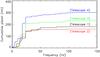 |
Fig. 3 Cumulative piston modeled for each telescope for the high vibration level. |
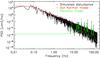 |
Fig. 4 PSD of a disturbance sequence on telescope 1 (black) and models used for the simulation: Von Kármán model for the atmospheric piston (red), and vibration model for the high vibration level (green). |
The maximum coherent flux Fmax coming to the input of each fiber during one frame is computed for the whole K band by 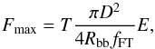 (6)with D the diameter of the telescope, Rbb the broad-band spectral resolution in the K band, fFT the frame rate, and T the overall transmission of the system, from the primary mirror to the detector (i.e., beam combiner transmission and detector quantum efficiency included).
We simulated an overall transmission of 1% as expected with the GRAVITY instrument and the VLTI facility. This leads to a typical flux of 400 photons per aperture and per frame at the input of the beam combiner for a magnitude K = 10 star, a telescope diameter of 8.2 m, and a loop frequency of 300 Hz.
2.2.2. Fiber injection efficiency
The tip-tilt fluctuations leading to flux variations come from three different contributions: telescope vibrations, residual wavefront aberrations from the AO, and tilt errors from the beam relay and guiding system. We modeled the tilt vibrations on the telescopes by a pure sinusoidal vibration at frequency 18.1 Hz with random phases for each telescope, and a standard deviation of 5 mas. This vibration is indeed the dominant one observed in tip-tilt on VLT/NACO.
We modeled the residual tilt from the AO system as well as the tilt from guiding errors with the temporal PSD measured with the IRIS tilt sensor (Gitton et al. 2004; Gitton & Haguenauer 2008). We used the following empirical model for the spectrum SIRIS, deduced from past ESO measurements2: 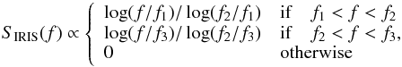 (7)with the cut-off frequencies f1 = 2 Hz, f2 = 8 Hz, and f3 = 50 Hz. We multiplied this model with the spectra of white Gaussian noise sequences to get random tilt sequences that are then scaled to standard deviations of 8.8 mas and 10.5 mas for the AO residuals and the guiding errors, respectively. Such values can be achieved at VLTI with a dedicated guiding camera that would stabilize the beams in the VLTI lab, as is planned for GRAVITY. The total tip-tilt sequences {θn} n ∈ [1,N] are computed from the sum of these three simulated tilt sequences.
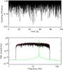 |
Fig. 5 Top: simulated coupling efficiency temporal sequence. Bottom: PSD of a tilt sequence (black), vibration added (green), and model used for AO and Guiding residuals (red). |
To compute the coupling ratio into the single-mode fibers, we assumed that the fiber coupler numerical aperture is optimized for the mode of the fibers. Following Wallner et al. (2002), the fiber mode field radius ω0 is then  (8)with fc the fiber coupler focal length. The coupling efficiency η for a beam tilted by an angle θ with respect to the optical axis is
  (9)with an optimum coupling efficiency η0 = 81% (without tilts and misalignments). We thus simulated the sequence {Fn}n∈[1,N] of coherent flux fluctuations such that
  (10)For a telescope of diameter D = 8.2 m, the average loss from optimal coupling is 80% with a standard deviation of 20%. A typical normalized flux sequence is presented in Fig. 5.
3. Simulation of the detection system
3.1. Acquisition sequence
To create a realistic acquisition temporal process in our simulator, we introduced a two-frame delay between the correction applied by the piston actuators and the corresponding effective disturbances. This takes one frame into account for the fringes to be acquired and one frame for the fringe tracker to compute the corresponding corrections, which are applied at the beginning of the next frame. This time scheme is illustrated in Fig. 6. The response of the actuators is assumed to be instantaneous at this point.
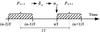 |
Fig. 6 Representation of the simulated discretized time scheme. At iteration n, the OPDs |

3.2. Beam combiner and detector
To properly estimate the residual OPDs (see Sect. 4.1), fringes are spectrally dispersed to efficiently compute large OPD residuals. In our simulations, the full K band is divided into Nλ = 5 spectral channels with effective wavelengths {λl}[1,Nλ] = {1.95 μm,2.075 μm,2.2 μm,2.325 μm,2.45 μm}.
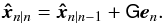
For each spectral channel l, the complex four-element amplitude vector  is computed at iteration n with phases resulting from the difference between the piston disturbances Pn and the piston actuator positions, i.e., the commands Un − 1 computed at the previous iteration:
 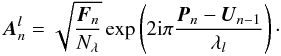 (11)To simulate the interferences, we used a pairwise ABCD beam combination with spatial coding (Benisty et al. 2009), where each couple of beams produces four intensities in phase quadrature (ABCD-like combination, Shao & Staelin 1977). This configuration is indeed optimal to sample fringes from four telescopes, as explained in Blind et al. (2011), and corresponds to the fringe sampling chosen for GRAVITY. In actual ABCD components, the measured modulations in phase opposition (A-C and B-D) are exactly 180° due to energy conservation, whereas the quadrature phase shifts are imperfect and weakly wavelength-dependent.
We simulated B-A phase shifts representative of measurements of the GRAVITY integrated optics beam combiner3, which are detailed in Table 6. They present departures from the nominal 90° phase shift from 2° to 17° and an average chromatic spread of 9.8°. In addition, we simulated a reduced contrast of 75% for each interference pattern, to account for overall contrast loss of the instrument, partial polarization effects, and OPD turbulence residuals.
The image generated by our simulator is a Nλ × 24 pixel dispersed image In where each row corresponds to one spectral channel. The 24-element intensity vector  at spectral channel l is computed thanks to the corresponding visibility-to-pixel matrix (V2PM), following the formalism developed by Lacour et al. (2008):
  (12)where V2PMl is the 24 × 16 V2PM matrix at spectral channel l, and
  is the 16-element vector of the coherences, defined in three parts such that
 ![Mathematical equation: \begin{equation} \vec{C}_n^l= \left[{\vec{C}_{F}}_n^l \quad \Re \left({\vec{C}_\mathrm{C}}_n^l\right) \quad \Im \left({\vec{C}_\mathrm{C}}_n^l\right)\right]^{\rm T}\label{eqCohVect}, \end{equation}](/articles/aa/full_html/2014/09/aa20223-12/aa20223-12-eq93.png) (13)with
(13)with  the four-element vector of the flux in each beam, defined for each aperture i by
  (14)and
  the six-element complex coherence vector, defined for each baseline k combining telescopes (i,j) by
  (15)Finally, two sources of noise are added to each pixel of the image In:
-
Photon noise, amplified by a factorFAPD = 1.5 to take the noise excess factor from an avalanche photo-diode detector (APD) into account;
-
Read-out noise of RON = 4 e− rms, amplified by a factor
 to account for a spread of the intensities over Npix = 2 detector pixels due to imperfect imaging optics.
These parameters are the characteristics of the SELEX-Galileo detector of the GRAVITY fringe tracker (Finger et al. 2010).
Simulated phase shifts of the B-A quadrature (nominal value of 90°) for the 6 baselines.
4. Description of the fringe-tracker algorithms
Fringe-tracking algorithms can be split into two equally important parts: the phase sensor, whose role is to provide accurate estimations of the OPD on all baselines, and the controller, which computes commands to the piston actuators out of these estimates. We provide a comprehensive description of the algorithms used in our simulations in this section.
4.1. OPD estimation
The six-baseline residual OPD vector  at time step n is computed from the last available image In − 1 (cf. Fig. 6). Two operators are used for its estimation.
The phase-delay operator (PD) estimates the OPD from the phase of the wide-band intensities. It provides an instantaneous estimation of the OPD, but modulo the wide-band wavelength (2.2 μm in the K band), and is thus alone insensitive to larger OPD fluctuations. To estimate the absolute OPD on each baseline, we thus use the group delay estimator (GD), which localizes the OPD of the maximum of the coherence envelope from the dispersed intensities.
4.1.1. Phase-delay estimation
For the PD estimation, we first compute the 24-element vector  of the wide-band intensities from the dispersed image:
  (16)Assuming that the beam combiner has been preliminarily characterized and that the wide band and dispersed V2PMs have been perfectly measured, the 16-element vector
  of the wide-band coherences is then estimated from the pixel-to-visibility matrix (P2VM) P2VMwb, pseudo-inverse matrix of the corresponding V2PM:
  (17)The residual PD OPD vector is deduced from the phase of the complex coherences
  , i.e., the 12 last elements of the wide-band coherence vector (see Eq. (13) for the structure of the coherence vector):
  (18)The resulting PD OPDs are thus computed modulo the effective wide-band wavelength λ0 = 2.2 μm in our simulations.
4.1.2. Group delay estimation
To estimate the position of the envelope of coherence with the GD estimator, the fringes are spectrally dispersed over Nλ spectral channels, and the group delay OPDs are estimated from the coherence measurements on these spectral channels. As the signal-to-noise ratio (S/N) of the synthetic wide-band intensities is increased by summing the Nλ spectral channels, we start by adding the last Nλ images available at iteration n to obtain an image  with an increased S/N:
  (19)The consequence of this operation is that the GD estimator does not measure the OPD at frame n − 1 but instead its average over the last five iterations.
To estimate the GD OPDs, we use an algorithm similar to the double Fourier interferometry used at IOTA (Pedretti et al. 2005). The 16-element coherence vector  is estimated at time step n for each spectral channel l using the calibrated P2VMl:
  (20)then the corresponding six-element complex coherent vector
  is extracted from its 12 last elements.
The cross-spectrum products between the complex coherences of each adjacent spectral channel are computed. The cross-spectrum product Xn(l1,l2) between channels l1 and l2 is defined by the element-wise product of the first one with the conjugate of the second one:  (21)Estimations of the group delay OPDs can be directly computed from the phase of each cross-spectrum product between adjacent spectral channels, within a range of Λ(l,l + 1):
  (22)where Λ(l,l + 1) is the beating wavelength between the spectral channels l and l + 1,
  (23)To increase the precision, we actually compute the GD OPD vector from the average of these Nλ − 1 individual GD OPD vectors:
 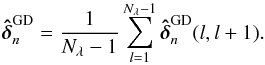 (24)This estimator becomes inaccurate as soon as the OPD is larger than ±min(Λ(l,l + 1))/2 because of the average of OPDs wrapped at different values. The fringe tracker needs to be designed with a spectral resolution enough to avoid such a problem happening within the range of variation of the OPD disturbance. For the fringe tracker of GRAVITY, the spectral resolution of R = 22 gives a range of validity of ± 16 μm for the group delay estimator, which is largely enough to measure for the OPD disturbance, all the more so because when the loop is closed, even if the tracking is lost during several iterations. In addition, with this wide range of validity, the GD OPD estimator can also be used to search for the fringes before closing the control loop, by moving the actuators over a long stroke, then starting the control with the actuators at positions close to the null OPDs.
4.1.3. Final OPD estimation
To solve for the ambiguity on the position of the fringe tracked by the PD estimator, we compute the final OPD  on each baseline k as
 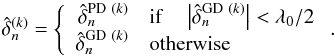 (25)The zero phase of the fringe is thus tracked except when a fringe jump occur, in which case the group delay is used to bring the fringes back to the maximum of coherence. The system is therefore stabilized to the zero phase of the central fringe, enabling long integrations on a dedicated separate science detector with no loss in the visibility accuracy and thus observation of faint targets.
4.2. OPD uncertainty estimation
For interferometer combining more than three telescopes, the redundancy between the closure phase relations (Jennison 1958) provides a simple way to verify that the estimated pistons are compatible all together when observing a unresolved target. If they are not, this redundancy can be used to improve their estimation by identifying the OPDs with the greatest uncertainty. The controllers implemented in our simulations and described in Sect. 4.3 make use of this particularity. To this purpose, the uncertainties on the OPDs also need to be estimated at each loop iteration.
For this, we first estimate the variance  on the intensity of each pixel of the last available image In − 1:
 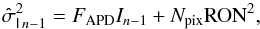 (26)an expression that takes the detector characteristics into account as described in Sect. 3.2. The first part of the equation corresponds to the photon noise amplified by the noise excess factor of the detector, and the second part corresponds to the detector read-out noise on Npix pixels. This variance map is then used to estimate the uncertainty for both PD and GD estimators.
4.2.1. PD OPD uncertainty
For the uncertainties on the PD estimations, we compute the 24 × 24 covariance matrix  of the wide-band intensities, assuming that the intensities are uncorrelated:
 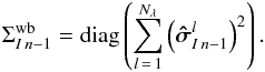 (27)We then deduce the covariance matrix of the wide-band complex coherence:
 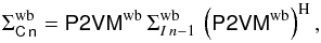 (28)where MH is the adjoint matrix of M. We select the variance
  of the complex coherence of the baseline k as the corresponding diagonal term of the covariance matrix:
  (29)The PD OPD uncertainty vector
  is finally estimated from the uncertainty
  on the phase of the complex coherence (see Appendix A for the derivation of the noise on the phase of the complex coherence):
  (30)
(30)
4.2.2. GD OPD uncertainty
Similarly, the covariance matrix  of the intensities of spectral channel l is computed from the sum of the Nλ last pixel noise estimations:
  (31)We then deduce the covariance matrix of the complex coherence of each spectral channel l:
 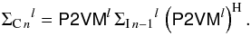 (32)The vector
  of the variance of the complex coherences is computed as the diagonal terms of this covariance matrix:
 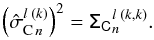 (33)The variance vector
  of the cross-spectrum product between each adjacent spectral channels l and l + 1 is derived as described in Appendix B.
The GD OPD variance vector is then computed from the average of the Nλ − 1 variances  of the phase of the cross-product between each adjacent spectral channels (see Appendix A for the derivation of the noise on the phase of the cross product):
 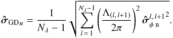 (34)
(34)
4.2.3. OPD uncertainty
Finally, the uncertainty on the estimation of the OPD on each baseline k is determined by selecting the uncertainty of the corresponding estimator, in the same way as we select the final OPD in Eq. (25):  (35)
(35)
4.3. OPD controllers
Once the OPDs and their uncertainties have been estimated on each baseline, they can be used and combined by the controller to compute optimal commands to be applied to the piston actuators and correct for the residual errors. In this section we describe the different controllers compared in our simulations: an integrator controller and a controller based on the Kalman algorithm.
4.3.1. Integrator controller
The integrator controller is implemented in two different schemes to investigate the better way to compute four piston commands from six estimated OPDs. In the first scheme (hereafter called OPD control scheme), commands are computed in baseline space to correct for the residual OPDs, then reverted to piston commands. In the second scheme (the piston control scheme), residual pistons are estimated from the estimated OPDs, then actuator commands are computed to correct for the piston residuals.
To account for the latency of the GD estimation resulting from the sum of Nλ previous images (Eq. (19)), two different integrator gains are used, KPD and KGD. The optimum gain on the baseline (k) is set such that 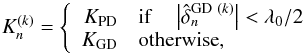 (36)defining Kn as the vector of gains on the six baseline. Then, KPD and KGD were preliminarily optimized with closed-loop simulations on a grid of values for both gains. We determined the optimal gain combination by minimizing the sum over all the baselines and the whole temporal sequence of the squared residual OPDs.
Moreover, to take advantage of the redundancy in the four telescope – six baseline architecture, weighted recombinations of the OPD residuals are computed from the estimated OPD uncertainties on the six baselines (Menu et al. 2012). If M is the 6 × 4 transfer matrix computing the six-element OPD vector from a four-element piston vector  :
:  (37)the weighted recombination of the OPDs is achieved by computing the weighted generalized inverse
  of the matrix M:
  (38)with the weight matrix Wn defined as the diagonal matrix of the inverse of the OPD variance vector
  :
:  (39)This weighted combination is used in both the OPD and piston scheme of the integrator controller.
OPD control scheme:
In this configuration, the weighted recombination of the OPDs  is first computed:
  (40)with the weighted identity matrix
  (41)OPD commands
  are then computed to compensate for these residual OPDs:
  (42)They are finally inverted to compute the piston commands Un:
  (43)
(43)
Piston control scheme:
In the aperture space control configuration, the residual piston vector is first deduced with the weighted inversion of the OPD vector :  (44)The correction Un of the integrator controller is then computed and sent to the piston actuators:
  (45)The matrix N converts the baseline gain vector Kn into an aperture gain vector by averaging the gain on the three baselines related to each aperture:
  (46)
(46)
4.3.2. Kalman controller
The Kalman filter is a recursive algorithm that can predict the new state of the disturbance based on a model of their evolution, which have to be identified beforehand, and from a set of previous measurements that are used to compare the prediction and the real measurements. From the estimation of the statistical characteristics of the disturbance, their evolution model, and the uncertainty on the measured residuals, control commands can be computed in a statistically optimal way.
The Kalman controller used in our simulations is very similar to the algorithm described in Menu et al. (2012), except for a few adaptations to our comprehensive case. We recall here the principle of the Kalman filter and give the details in which its implementation differs from this reference.
State-space formalism:
The formalism used by a Kalman filter is based on a couple of assumptions: the disturbance can be described by a set of independent components (typically the atmospheric piston and a discrete number of longitudinal vibrations for fringe-tracking systems) and the evolution each component can be described by an iterative linear model.
Here we follow the Meimon et al. (2010) statement that the evolution of both the atmospheric and the vibration components can be described by an autoregressive model of order two in the form:  (47)where
  is the vth component of the disturbance at time step n, the coefficients
  and
and  are computed from the component characteristics (natural frequency and damping coefficient, the later being lower than 1 for vibrations and greater than 1 for the atmospheric turbulence), and vn a white noise of standard deviation σv triggering the excitation of the component (see Meimon et al. 2010, for the derivation of the coefficients and ). In our simulated case, given Ncomp the total number of disturbance components, all baselines included, this evolution model can be generalized to the following matrix form:
  (48)where xn is a 2Ncomp-element vector describing the state of each component at iteration n and n − 1, A is the 2Ncomp × 2Ncomp matrix gathering the a1 and a2 coefficients of every component, and vn is the 2Ncomp-element vector of the excitation noises.
The OPD vector measured at iteration n is related to the state vector by the 6 × 2Ncomp matrix C (which sums the  components related to each baselines in the state vector xn), the OPDs induced by the actuator positions, and the measurement noise at iteration n:
  (49)
(49)
Control algorithm:
Assuming that the evolution model of the OPD disturbance has been preliminarily identified (i.e., the matrices A, C and the excitation noises), the Kalman controller algorithm consists of four successive steps:
-
1.
We compute the error en between the OPDs
 estimated at iteration n and the OPDs predicted at the previous iteration by the Kalman controller. The latter results from the effective actuator positions delayed by two iterations (see Fig. 6) and from the disturbance state
  predicted by the controller for iteration n based on all observations up to iteration n − 1:
 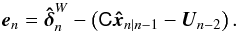 (50)
(50) -
2.
The state vector is then updated with this correction vector and the Kalman gain matrix G:
 (51)
(51) -
3.
The next state of the disturbance is predicted using the evolution model defined by matrix A:
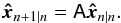 (52)
(52) -
4.
The command vector Un to the actuators is finally computed by inverting the optimal OPD commands to optimal piston commands, with the respective matrices K and
 :
: 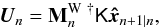 (53)with K a 6 × 2Ncomp matrix, which sums the
  components related to each baselines in the state vector
  .
.
The Kalman gain G is a 2Ncomp × 6 weight matrix that determines how much confidence in the theoretical model we have with respect to real measurements. It is statistically optimal when computed as follows, knowing the OPD uncertainties and the disturbance excitations:  (54)with Σ∞ the solution of the Riccati equation,
  (55)where Σv is the 2Ncomp × 2Ncomp covariance matrix of the excitation noise of the disturbance components, simply a diagonal matrix in our system, with the σv terms at the positions and zero terms at the positions, and Σw is the covariance matrix of the OPD measurement noise. Since the OPDs are estimated from two different estimators (Eq. (25)), we used two different measurement noise covariance matrices Σw, computed with a similar weighted combination as for the OPDs. We thus used two different Kalman gain matrices, optimized for phase and group delay OPD measurements, respectively, the proper gain for each baseline being selected the same way as in Eq. (25).
Model identification:
To identify the evolution model of the disturbance, a sequence of OPDs representative from the variations has to be measured before tracking the fringes with the Kalman controller. To do so, we used a similar approach than those described in Menu et al. (2012) and Meimon et al. (2010), with a few adaptations to our case.
Because of the large OPDs induced by the atmospheric disturbance, open-loop measurements cannot be obtained without losing the fringes. Instead, a pseudo-open loop (POL) OPD sequence has to be computed by tracking the fringes with a classical controller to measure the OPD residuals with high precision, then reconstructing the corresponding disturbance sequence knowing the actuator positions. In our simulations, we computed POL sequences by performing short fringe-tracking simulations with the piston scheme integrator controller described in Sect. 4.3.1. To compute the POL OPD sequence, we used the OPDs estimated in Eq. (25), the actuator commands computed in Eq. (45), and the weighted identity matrix computed in Eq. (41) to have estimates of the POL OPDs improved by the redundant configuration of instrument:  (56)From these POL sequences, we used the same method as in Menu et al. (2012) to identify the disturbance components and their evolution model and computed the matrices A, Σv, C, and K. The measurement covariance matrices Σw for the phase delay and group delay estimators are also computed from the POL OPD sequences.
5. Results of the simulations
The performances of the integral and of the Kalman controllers were simulated for different star magnitudes, observing conditions, and loop frequencies. The varying parameters are summarized in Table 2. Both versions (piston and OPD scheme) of the integral controller were simulated, and the disturbance model used for the Kalman controller was identified with POL sequences of four different lengths.
To improve the statistics on the results, each simulation is performed ten times with different random disturbance sequences for each baseline4. The sequences of true OPD residual are computed for each baseline and each realization as the difference between the simulated disturbance sequence and the sequence of OPDs applied by the piston actuators. These positions correspond to the vector Un computed in Eqs. (43), (45), and (53) with one iteration of delay (see Fig. 6). The standard deviations of these sequences5 over time are then computed and the performance of the controllers is judged with the median of these standard deviations over the six baselines and the ten random realizations (thus median over 60 observables).
In the following, we present results at the loop frequency minimizing these standard deviation of the OPD residuals. The optimal frequencies are also presented for each star magnitude, each controller, and observing conditions. They provide the best compromise between the controller bandwidth and accuracy of the OPD estimation depending of the reference star magnitude.
5.1. Performances at different vibration levels
We analyzed the performances of the controllers by simulating three different vibration levels: no longitudinal vibration, a low vibration level corresponding to the one expected at VLTI in late 2014 (150 nm rms OPD on each baseline), and a high vibration level similar to the one currently estimated at VLTI on the UTs (cf. Tables 4 and 5). The residual OPDs at optimal loop frequency are presented in Fig. 7 as a function of magnitude for each vibration levels and the corresponding optimal frequencies are presented in Fig. 8. Flux variations resulting from 15 mas rms residual tip-tilt and atmospheric turbulence with 10 μm rms OPD were simulated for each case.
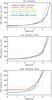 |
Fig. 7 OPD residuals as a function of magnitude for three different vibration levels. Top: no vibration; middle: low vibration level with 150 nm rms OPD; bottom: high vibration level from 240 to 380 nm rms OPD. The atmospheric turbulence is 10 μm rms OPD and, and the residual tip-tilt of the beams is 15 mas rms. The dashed lines correspond to the specification of the fringe tracker of GRAVITY, which is to stabilize the fringes down to 350 nm rms on a reference star of magnitude K = 10. |
For reference stars brighter than K ~ 9.5, the piston and OPD schemes of the integrator are equally efficient, for the three vibration levels. The piston scheme integrator is more robust to fainter magnitudes and presents a gain of a few hundred nanometers rms over the OPD scheme.
Without vibrations (Fig. 7, top), the Kalman controller and the piston scheme integrator have very similar performances, regardless of the magnitude. For the simulated flux variation level, both controllers are thus equally efficient at compensating for the atmospheric disturbance. In addition, with 10 μm rms of atmospheric OPD, a 2000-frame POL sequence is as efficient as longer ones and is then enough to properly identify the turbulence component in the disturbance even at low S/N.
At high S/N, the Kalman controller is mainly insensitive to the vibration level, unlike the integrator controllers. For stars brighter than K ~ 8, the OPD residuals with the Kalman controller are stable to 100 ± 50 nm rms whatever the vibration level, whereas the performance of the integrator controller clearly scales with the vibration level. The Kalman controller is thus very efficient at canceling out the vibrations in this regime. In addition, at high S/N, a 2000-frame POL sequence is enough to properly identify and calibrate the vibrations that we simulated. If the system presents vibrations with lower frequencies, longer POL sequences might, however, be needed to properly characterize their evolution model. Performances of all controller are limited by the maximum simulated loop frequency of 1 kHz (see Fig. 8). Using a higher loop frequency in this case may actually improve the fringe stabilization by increasing the bandwidth of the controller.
In a medium S/N regime, the performances of all controllers continuously decrease, because the estimated OPDs are less accurate and the error on the piston commands are then greater. The Kalman controller still stabilizes the fringes better than the integrator thanks to its predictive algorithm, which optimally weights predictions from the disturbance model and measured OPD residuals. However, it becomes slightly less efficient in this regime than at high S/N because the state vector is updated with measurements of poor precision, and because the disturbance model is identified from POL sequences where the fringes were stabilized with a classical integrator, which is not very efficient in the mid-S/N regime. The disturbance sequences reconstructed from the estimated OPD residuals are not as accurate as when the fringes are efficiently stabilized, and the disturbance components are not properly characterized. This is particularly observable in the presence of strong vibrations for two principal reasons. First, a high level of vibrations significantly increases the total OPD fluctuations and leads to poor fringe tracking during the POL sequence, hence to an even less accurate disturbance model. Second, the sharper the vibration, the more precise its identification must be to provide accurate control. For very narrow-band components (k ≪ 1), a slight error in its characterization (e.g., its natural frequency) can lead to a poor compensation. On the contrary, the atmospheric disturbance is properly corrected by the Kalman controller even at very low S/N (see Fig. 7, top), because its model with a large damping coefficient k makes its identification very robust to large uncertainties.
At low S/N, the Kalman controller becomes less robust than the integrator controller if there are vibrations in the system. With OPD residuals greater than 500 nm rms with the integrator controller, the reconstructed POL sequences are not accurate enough to provide a proper model identification for the vibrations, and the Kalman controller cannot converge to correct commands. In addition, at low S/N the controller loop frequency lower than 400 Hz for magnitudes above 9.5 makes identification of vibrations with high frequency more difficult.
The performances of the Kalman controller slightly improve if the length of the POL sequence is increased. The longer the POL sequence, the better the precision for identifying of the disturbance components. However, using longer POL sequences may reveal itself to be useless in practice: the disturbances may possibly vary during the observation, and short POL sequences are less subject to model variations. In our simulations, we assume temporally invariant disturbances, but we discuss this possibility in Sect. 6.
5.2. Performances at different flux variation levels
When working at the sensitivity limit of a fringe tracker, flux variations are a serious cause of performance loss with classical controllers: if the flux in one beam drops too low to accurately estimate the OPDs with a sufficient precision (called a flux dropout hereafter), incorrect or no commands at all are sent to the actuator. The typical sources of flux variations for single-mode fibered interferometer are the residual wavefront errors from the AO systems, telescope tip-tilt vibrations, and tip-tilt errors from the guiding system.
We analyzed the robustness of the controllers to flux dropouts by simulating a residual tip-tilt jitter of the beams with two different levels: the nominal level of 15 mas rms, as expected for GRAVITY after guiding correction, and a high tip-tilt level of 20 mas rms. The residual OPDs at optimal loop frequency are presented in Fig. 9 as a function of magnitude for 20 mas rms tip-tilt variations, with OPD vibrations of 150 nm rms and atmospheric disturbance of 10 μm rms. The corresponding optimal frequencies are presented in Fig. 10.
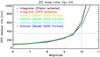 |
Fig. 9 OPD residuals as a function of magnitude, with flux variations due to 20 mas rms residual tip-tilt jitter. The OPD disturbances are 10 μm rms atmospheric OPD and 150 nm rms vibration OPD (low vibration level). The dashed lines correspond to the specification for the fringe tracker of GRAVITY, which is to stabilize the fringes below 350 nm rms on a reference star of magnitude K = 10. |
At high S/N (up to magnitude 8), the Kalman and the integrator controllers are equally insensitive to flux variations, and the OPD residuals are hardly more with 20 mas than with 15 mas rms residual tip-tilt (cf. Fig. 7, middle panel). Actually in this regime, the star magnitude is far from the sensitivity limit of the instrument, and flux variations only result in variations in the precision of the OPD, which are compensated by the weighted OPD combination provided by the redundant architecture of the interferometer (see Sects. 4.2 and 4.3).
At low S/N, both controllers are almost equally robust to flux dropouts. Their performances as a function of magnitude are shifted a quarter of a magnitude between the two simulated tip-tilt levels. With a faint reference star close to the sensitivity limit of the instrument, flux variations induce frequent flux dropouts. The efficiency of the Kalman controller depends on the quality of the disturbance model, consequently on the integrator controller accuracy. The predictive power of the Kalman filter is thus inhibited by the poor quality of the model at low S/N, and the Kalman controller is no more robust than the integrator controller.
5.3. Performances at different atmospheric OPD levels
We also analyzed the robustness of the controllers to a stronger atmospheric turbulence. In addition to the nominal level of 10 μm rms atmospheric OPD, we then simulated the atmospheric turbulence of 15 μm rms. It corresponds to 1′′ and 1.7′′ seeing, assuming a Von Kármán model with a 100 m outer scale (Conan et al. 2000). The residual OPDs for 15 μm atmospheric turbulence are presented in Fig. 11, with 150 nm rms vibrations and 15 mas rms residual tip-tilt of the beams. The corresponding optimal frequencies are presented in Fig. 12.
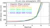 |
Fig. 11 OPD residuals as a function of magnitude with an atmospheric OPD of 15 μm rms. The vibration level is 150 nm rms per baseline (low vibration level), and the flux variations are due to 15 mas rms beam tip-tilt variations.The dashed lines correspond to the specification for the fringe tracker of GRAVITY that is to stabilize the fringes below 350 nm rms on a reference star of magnitude K = 10. |
The performances of each controller as a function of magnitude are noticeably similar for both disturbance levels (compare to Fig. 7, middle panel). With a bright reference star, the controllers are insensitive to the atmospheric piston, thanks to the system redundancy, which improves the OPD estimations (see Sects. 4.2 and 4.3). The impact of a stronger atmospheric turbulence is to lower the sensitivity limit of the fringe tracker by half a magnitude for all controllers. The Kalman controller is not significantly more robust than the integrator controller for these observing conditions.
5.4. Kalman model identification on a bright star
From the results presented above, we conclude that the performance of the Kalman controller is mainly limited in the low S/N regime by inaccuracies in the identification of the model of the vibrations, owing to a poor fringe stabilization during the POL sequences by the integrator controller. To overcome this limitation, we investigated the possibility of tracking the fringes on a bright star during the POL sequence to improve the disturbance model identification and the Kalman controller performance on the faint reference star.
We thus performed additional simulations in which the POL sequences are acquired on a bright star of magnitude K = 7 with the piston scheme integrator controller. Assuming that the bright star and the faint reference star are close to each other (within a few degrees) and that the telescope slew is fast enough, the light coming from the two stars is subject to atmospheric turbulence with similar statistical properties and similar vibrations with telescopes pointing in very close directions, so the same disturbance model can be used. Only the Kalman gain matrix (Eq. (54)) has to be adapted to optimally track the fringes on the faint reference star. For this we computed the Kalman gain with OPD uncertainties estimated from POL sequences simulated with the faint reference star.
For this analysis, we only ran simulations in the mid- and low-S/N regime, with reference star magnitudes ranging from 9 to 11 and loop frequencies from 100 to 500 Hz. The OPD residuals obtained with 10 μm rms atmospheric turbulence and 15 mas rms tip-tilt variations are presented in Figs. 13 and 14 for the low and high vibration levels, respectively. The corresponding optimal loop frequencies are presented in the top and bottom panels of Fig. 15.
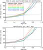 |
Fig. 13 OPD residuals as a function of magnitude for 10 μm rms atmospheric OPD, for 15 mas rms residual tip-tilt variations, and for the low vibration level (150 nm rms vibration OPD). Top: disturbance model is computed from a POL sequence acquired on the star itself (it is simply a zoom-in of Fig. 7, middle panel). Bottom: the model is computed observing a bright object (K = 7). The dashed lines correspond to the specification for the fringe tracker of GRAVITY which is to stabilize the fringes below 350 nm rms on a reference star of magnitude K = 10. |
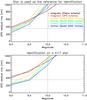 |
Fig. 14 Same as Fig. 13, except that the simulations were done for the high vibration level (240 to 380 nm rms OPD). The top panel is here a zoom-in of Fig. 7, bottom panel). |
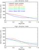 |
Fig. 15 Optimal frequencies as a function of the magnitude for conditions when the disturbance model is identified on a star of magnitude K = 7. Top panel is related to Fig. 13 and bottom panel to Fig. 14. |
For the low vibration level (Fig. 13), there is slight improvement in the performance of the Kalman controller when identifying the disturbance model on high-S/N POL sequence, in particular for magnitude greater than 10. For stars brighter than K = 10, the performances are mostly limited by the measurement noise level and by the flux dropouts rather than by the accuracy of the model and the gain in the OPD stabilization is of only a few tens of nanometers.
For stronger vibrations (Fig. 14), the identification of the disturbances with high-S/N POL sequences clearly improves the Kalman controller performances. At magnitude 10, the OPD residuals are lowered by 250 nm rms by identifying the disturbances model with a K = 7 star. Actually, at low S/N, the vibration level is too high for the integrator to properly track the fringes during the POL sequence (OPD residuals of 820 nm rms at magnitude 10), and the disturbance model estimated from these measurements is not accurate enough to provide efficient fringe tracking with the Kalman controller. On the other hand, with a model identified from high-S/N POL sequences, the control with the Kalman filter is then only limited by the flux dropouts.
6. Discussion
In this section we discuss the limitations of our simulations. We also analyze these results for the particular case of GRAVITY that we used as the framework for our simulations, and we discuss their impact on the objectives of the instrument.
6.1. Limits on the simulations
First of all, our simulations of the atmospheric turbulence are based on a Von Kàrmàn model and parameters qualitatively chosen to generate disturbance sequences and spectra similar to those measured at VLTI. This model significantly differs from the one used at VLT to describe median observing conditions, based on a Kolmogorov model. According to this model, our simulations might be too optimistic when simulating 10 μm rms OPD, whereas 15 μm rms OPD would correspond to the median conditions. The median atmospheric piston is characterized at VLTI by 310 nm rms OPD variations on a timescale of 48 ms when using a Kolmogorov model, which is the level we obtain by simulating a total turbulence level of 15 μm rms with the Von Kàrmàn model. However, the metric defining the median atmospheric conditions might differ for the two models since the Kolmogorov model diverges at zero frequency and leads to a total piston variation depending on the time scale, unlike for a Von Kàrmàn model.
The second limitation of our simulation is that we simulated an instantaneous response for the piston actuators, which is not realistic when working at high loop frequencies, hence for bright reference stars in the high S/N regime. Limited actuator bandwidths will reduce the absolute performance of all controllers but should not change the conclusion on the relative performance of the Kalman controller with respect to the integrator. In addition, the algorithm of the Kalman controller can be adapted to limited actuator bandwidths, as described by Correia et al. (2010), to improve the controller performance. In the specific case of GRAVITY, the piston actuators of the fringe tracker will have a 3 dB bandwidth of 220 Hz. We thus anticipate a small loss in performances in fringe tracking on reference sources brighter than K = 8.5 whose optimal frequency is greater than 500 Hz.
Finally, we considered time-invariant disturbances in our simulations. However, the atmospheric seeing slowly varies on time-scales of a few minutes, and realistic instrumental vibrations may have varying frequency or amplitude, changing with, for instance, the wind speed or orientation, or the telescopes pointing. If these variations are very significant, the disturbance model used for the Kalman filter has to be updated regularly on time scales of 5−10 s to efficiently correct vibrations. For this, POL sequences can be reconstructed directly from tracking sequences using the Kalman controller, and the updated disturbance model can be computed on a dedicated computer without stopping the control loop. Since the Kalman controller is better at stabilizing fringes than a classical controller, the new POL sequences will have better precision than the initial one obtained with the integrator controller, and the disturbance model will not only be updated for the vibrations, but also be more accurate for the atmospheric turbulence. This strategy may be particularly valuable if the initial model has been identified by tracking the fringes on a bright star before Kalman-tracking on the faint reference star (see Sect. 5.4). Updating the initial model with new POL sequences acquired on the faint reference star would actually remove potential biases from the small angular separation between the bright initial star and the tracking reference star, if the atmospheric turbulence is not statistically spatio-temporally invariant.
6.2. Performances with respect to GRAVITY
To enable the observation of the Galactic center, GRAVITY will use IRS16C as the reference for the fringe tracker, a star of magnitude K = 9.7. To achieve its science objectives, the fringe tracker is required to be able to track fringes down to 350 nm rms on a K = 10 reference source with the UTs, assuming vibrations below 150 nm rms OPD, 15 mas rms residual tip-tilt per beam, and median seeing conditions. Moreover, fringe tracking down to 300 nm rms OPD must be achieved without vibrations in the same observing conditions, assuming that OPD vibrations will incoherently add to the residuals.
OPD residuals at magnitude 10, with 150 nm rms OPD vibrations, 10 μm rms atmospheric OPD, 15 mas rms residual tip-tilt per beam.
OPD residuals at magnitude 10, without longitudinal vibrations, 10 μm rms atmospheric OPD, 15 mas rms residual tip-tilt per beam.
Our simulations show that a Kalman controller will enable the fringe tracker of GRAVITY to meet these requirements, but not an integrator controller. The OPD residuals for each controller for fringe tracking at magnitude 10 under the specified conditions are detailed in Table 7. The use of a long POL sequence of 5000 frames to identify the disturbance model provides a 40 nm rms margin to the specified OPD residual level, at the cost of memory and computation time for identifying the model.
Without vibrations, the Kalman algorithm also provides better control than the integrator controller, although both algorithms reach the specification of the fringe tracker of GRAVITY. The corresponding OPD residuals are given in Table 8. The Kalman controller provides ~70 nm rms margin to the specified OPD residual level.
However, these performances at magnitude 10 are close to the limits of the Kalman controller. They quickly degrade with stronger disturbances: the fringe tracker sensitivity is lowered by half a magnitude for 20 mas rms tip-tilt of the beams or for 15 μm rms atmospheric OPD. More effort to damp the vibration level at VLTI is also crucial for GRAVITY to reach its science objectives. With the current vibration level on the UTs, fringe tracking at magnitude 10 cannot be expected to provide OPD residuals lower than 800 nm rms, and the 350 nm rms residual level can only be reached with a K = 9.2 star.
7. Conclusion
In this paper, we studied the performances of two different algorithms to track fringes with an interferometer. We performed simulations of fringe tracking with different reference star magnitude, with realistic disturbances based on observing conditions at VLTI (flux variations, vibrations, and seeing conditions) and compared the performances obtained with an optimized integrator controller and with a controller based on a Kalman filter, which can predict statistically optimal commands based on a model of the disturbance. We based our simulations on the architecture and design of the GRAVITY instrument, a four-telescope combiner that will be installed at VLTI end of 2014.
In the high S/N regime, we found that the efficiency tracking fringes is constant for each controller. Their performance is limited by the maximal loop frequency that the system can achieve (1 kHz in our simulations), and thus by the controller bandwidths. In the presence of vibrations, the Kalman controller is significantly more efficient than an integrator controller at high S/N. Whereas the integrator controller is clearly limited by the vibrations, the Kalman controller is almost insensitive to the vibration level and more generally to the disturbance level in this range of magnitude. The disturbance model is accurately estimated and the actuator commands are computed with accurate prediction of the vibrations.
At lower S/N, the performances of both controllers significantly decrease with the star magnitude. For the Kalman controller, supposed to be able to predict optimal commands, it can be attributed to an inaccurate model of the disturbances. Because of poor-efficiency fringe tracking with the integrator controller during the preliminary sequence used to calibrate the disturbances, the model of disturbance used by the Kalman controller is indeed not accurately estimated, and the corrections are not properly adapted. For observing conditions leading to OPD residuals of more than ~λ/ 4 with the integrator controller (faint magnitude, high disturbance, or flux dropout level), the noise on the preliminary sequence is too important to provide an accurate identification of the disturbance model and the Kalman controller is less robust than a classical integrator controller.
We also found that in this situation, the piston control can be improved by identifying the disturbance model from high S/N preliminary sequences using a bright star with the integrator controller before tracking the fringes on the faint reference star with the Kalman controller.
Finally, our results show that the VLTI instrument GRAVITY will be able to reach its science objectives with a fringe tracker using a Kalman controller, by stabilizing the fringes down to 350 nm rms with a reference star of magnitude K = 10 under median atmospheric conditions. However, this performance depends on a significant effort to mitigate vibration at VLTI down to 150 nm rms OPD on the UTs. Four-telescope fringe tracking is to be demonstrated with both algorithms in laboratory during the integration of GRAVITY in mid-2014, then on sky by 2015.
Developed in the Interactive Data Language (IDL) programming language.
Philippe Gitton (priv. comm.).
Laurent Jocou (priv. comm.).
The typical computation time for one realization is about 1h for simulations with every controller (two integrator and Kalman controller with four different POL-sequence lengths) at a given star magnitude and loop frequency on a 8-core 2.27 GHz Intel Xeon machine. Our simulator is a high-level research tool intended to test fringe-tracking algorithms, and it has not been optimized for computation celerity.
The first 1000 iterations are excluded from the standard deviation computation to account for the time needed by the controller to converge.
Acknowledgments
We are grateful to Cyril Petit and Serge Meimon for initial discussions and advice on Kalman/LQG control, and to Julien Lozi for discussions on practical implementation of the Kalman algorithm. We also thank Jean-Marc Conan, Caroline Kulcsar, and Henri-François Raynaud for substantial suggestions on state-of-the-art of Kalman/LQG command for adaptive optics. EC is grateful to the DGA and CNRS/INSU for a PhD fellowship grant.
References
- Benisty, M., Berger, J.-P., Jocou, L., et al. 2009, A&A, 498, 601 [NASA ADS] [CrossRef] [EDP Sciences] [Google Scholar]
- Berger, D. H., Monnier, J. D., Millan-Gabet, R., et al. 2008, Proc. SPIE, 7013, 701319 [CrossRef] [Google Scholar]
- Blind, N., Absil, O., Le Bouquin, J.-B., Berger, J.-P., & Chelli, A. 2011, A&A, 530, A121 [NASA ADS] [CrossRef] [EDP Sciences] [Google Scholar]
- Buscher, D. F., Armstrong, J. T., Hummel, C. A., et al. 1995, Appl. Opt., 34, 1081 [NASA ADS] [CrossRef] [Google Scholar]
- Campins, H., Rieke, G. H., & Lebofsky, M. J. 1985, AJ, 90, 896 [NASA ADS] [CrossRef] [Google Scholar]
- Colavita, M. M., Booth, A. J., Garcia-Gathright, J. I., et al. 2010, PASP, 122, 795 [NASA ADS] [CrossRef] [Google Scholar]
- Colavita, M. M., Wizinowich, P. L., Akeson, R. L., et al. 2013, PASP, 125, 1226 [NASA ADS] [CrossRef] [Google Scholar]
- Conan, R., Ziad, A., Borgnino, J., Martin, F., & Tokovinin, A. A. 2000, Proc. SPIE, 4006, 963 [NASA ADS] [CrossRef] [Google Scholar]
- Correia, C., Raynaud, H.-F., Kulcsár, C., & Conan, J.-M. 2010, J. Opt. Soc. Am. A, 27, 333 [NASA ADS] [CrossRef] [Google Scholar]
- Dali Ali, W., Ziad, A., Berdja, A., et al. 2010, A&A, 524, A73 [NASA ADS] [CrossRef] [EDP Sciences] [Google Scholar]
- Delplancke, F., Derie, F., Lévêque, S., et al. 2006, Proc. SPIE, 6268, 62680 [CrossRef] [Google Scholar]
- Di Lieto, N., Haguenauer, P., Sahlmann, J., & Vasisht, G. 2008, Proc. SPIE, 7013, 70130 [CrossRef] [Google Scholar]
- Eisenhauer, F., Perrin, G., Brandner, W., et al. 2011, The Messenger, 143, 16 [NASA ADS] [Google Scholar]
- Finger, G., Baker, I., Dorn, R., et al. 2010, Proc. SPIE, 7742, 77421 [Google Scholar]
- Gillessen, S., Eisenhauer, F., Perrin, G., et al. 2010, Proc. SPIE, 7734, 77340 [CrossRef] [Google Scholar]
- Gitton, P., & Haguenauer, P. 2008, Proc. SPIE, 7013, 70130 [CrossRef] [Google Scholar]
- Gitton, P. B., Leveque, S. A., Avila, G., & Phan Duc, T. 2004, Proc. SPIE, 5491, 944 [NASA ADS] [CrossRef] [Google Scholar]
- Haguenauer, P., Alonso, J., Bourget, P., et al. 2010, Proc. SPIE, 7734, 04 [Google Scholar]
- Haguenauer, P., Abuter, R., Andolfato, L., et al. 2012, Proc. SPIE, 8445, 84450 [Google Scholar]
- Hartung, M., Macintosh, B., Poyneer, L., et al. 2013, in Proc. of the 3d AO4ELT Conference, eds. S. Esposito, & L. Fini, id. 116 [Google Scholar]
- Jennison, R. C. 1958, MNRAS, 118, 276 [NASA ADS] [CrossRef] [Google Scholar]
- Kalman, R. E. 1960, Trans. ASME-J. Basic Eng., 82, 35 [Google Scholar]
- Lacour, S., Jocou, L., Moulin, T., et al. 2008, Proc. SPIE, 7013, 16 [NASA ADS] [Google Scholar]
- Lane, B. F., & Muterspaugh, M. W. 2004, ApJ, 601, 1129 [NASA ADS] [CrossRef] [Google Scholar]
- Le Bouquin, J.-B., Abuter, R., Bauvir, B., et al. 2008, Proc. SPIE, 7013, 7 18 [Google Scholar]
- Le Roux, B., Conan, J.-M., Kulcsár, C., et al. 2004, J. Opt. Soc. Am. A, 21, 1261 [NASA ADS] [CrossRef] [Google Scholar]
- Lozi, J., Cassaing, F., Le Duigou, J.-M., et al. 2011, Proc. SPIE, 8151, 81510B [CrossRef] [Google Scholar]
- Maire, J., Ziad, A., Borgnino, J., et al. 2006, A&A, 448, 1225 [NASA ADS] [CrossRef] [EDP Sciences] [Google Scholar]
- Martin, F., Conan, R., Tokovinin, A., et al. 2000, A&AS, 144, 39 [NASA ADS] [CrossRef] [EDP Sciences] [Google Scholar]
- Meimon, S., Petit, C., Fusco, T., & Kulcsar, C. 2010, J. Opt. Soc. Am. A, 27, A122 [NASA ADS] [CrossRef] [Google Scholar]
- Menu, J., Perrin, G., Choquet, E., & Lacour, S. 2012, A&A, 541, A81 [NASA ADS] [CrossRef] [EDP Sciences] [Google Scholar]
- Mérand, A., Patru, F., Berger, J.-P., Percheron, I., & Poupar, S. 2012, in SPIE Conf. Ser., 8445 [Google Scholar]
- Müller, A., Pott, J.-U., Morel, S., et al. 2010, Proc. SPIE, 7734, 20 [NASA ADS] [Google Scholar]
- Pedretti, E., Traub, W. A., Monnier, J. D., et al. 2005, Appl. Opt., 44, 5173 [NASA ADS] [CrossRef] [PubMed] [Google Scholar]
- Petit, C. 2006, Ph.D. Thesis, Université Paris 13 [Google Scholar]
- Petit, C., Quiros-Pacheco, F., Conan, J.-M., et al. 2004, Proc. SPIE, 5490, 1414 [NASA ADS] [CrossRef] [Google Scholar]
- Petit, C., Sauvage, J.-F., Sevin, A., et al. 2012, Proc. SPIE, 8447, 84471Z [Google Scholar]
- Poupar, S., Haguenauer, P., Merand, A., et al. 2010, Proc. SPIE, 7734, 37 [NASA ADS] [Google Scholar]
- Ragland, S., Akeson, R., Colavita, M., et al. 2010, Proc. SPIE, 7734, 02 [Google Scholar]
- Reinhardt, G. W., & Collins, S. A. J. 1972, J. Opt. Soc. Am., 62, 1526 [CrossRef] [Google Scholar]
- Sahlmann, J., Ménardi, S., Abuter, R., et al. 2009, A&A, 507, 1739 [NASA ADS] [CrossRef] [EDP Sciences] [Google Scholar]
- Shao, M., & Staelin, D. H. 1977, J. Opt. Soc. Am., 67, 81 [Google Scholar]
- Shao, M., & Staelin, D. H. 1980, Appl. Opt., 19, 1519 [NASA ADS] [CrossRef] [EDP Sciences] [Google Scholar]
- Sivo, G., Kulcsar, C., Conan, J.-M., et al. 2013, in Proc. of the 3d AO4ELT Conference, eds. S. Esposito, & L. Fini, 127 [Google Scholar]
- Wallner, O., Winzer, P. J., & Leeb, W. R. 2002, Appl. Opt., 41, 637 [NASA ADS] [CrossRef] [Google Scholar]
- Williams, D. F., Wang, C. M., & Arz, U. 2006, in ARFTG Conf. Dig., 68 [Google Scholar]
Appendix A: Derivation of the noise of the phase
Let V be a complex visibility of phase and modulus φ and | V |, respectively, in the complex plane. Let σV = (σx,σy) be the noise on V in the complex plane, with σx and σy the real and imaginary parts, respectively. Assuming that the noise are not correlated, the noise on the complex vector V is thus described by an ellipse of semi-minor axis σx and semi-major axis σy in the basis (V,ℑ,ℜ) centered on V (see Fig. A.1). A point on the ellipse with coordinates (x,y) in this basis verifies the equation  (A.1)In the radial orthonormal basis (V,V∥,V⊥) defined respectively by the axis parallel and orthogonal to V, the same point of coordinates (u,v) verifies the equation
  (A.2)The noise σφ on the phase can be approximated by the differential phase between the V and the point of the ellipse whose partial derivative in u is null (which corresponds to the point of maximum coordinate on the axis B⊥). Two points verify these relations, with coordinates (u1,v1) and (u2,v2) in the basis (V,V∥,V⊥):
 The noise σφ on the phase is thus
  (A.5)This expression neglects the covariance terms between the real and the imaginary parts of the complex vector. We refer to Williams et al. (2006) for the analytical expression for the noise on the phase in case of correlation between both measurements.
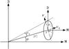 |
Fig. A.1 Representation of the complex visibility V and of the noise σVin the complex plane (V,ℜ,ℑ) and in the radial basis (V,V∥,V⊥). |
Appendix B: Derivation of the noise of the cross-product operator
The cross-product operator for a single baseline can be expressed as a function z of two complex numbers x and y:  (B.1)The expression of the real and imaginary parts of z are developed respectively as
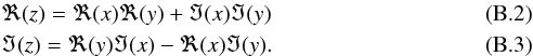 The variance of these expressions is expressed respectively as
 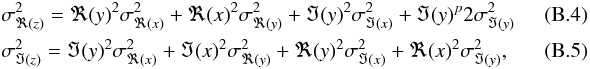 with
with  and
and  , the variance of the real and imaginary parts of x, respectively.
All Tables
Simulated phase shifts of the B-A quadrature (nominal value of 90°) for the 6 baselines.
OPD residuals at magnitude 10, with 150 nm rms OPD vibrations, 10 μm rms atmospheric OPD, 15 mas rms residual tip-tilt per beam.
OPD residuals at magnitude 10, without longitudinal vibrations, 10 μm rms atmospheric OPD, 15 mas rms residual tip-tilt per beam.
All Figures
|
Fig. 1 Comparison of Kolmogorov and Von Kármán models with different atmospheric outer scale values. Top: standard deviation of OPD fluctuations as a function of the baseline length for median atmospheric conditions in the K band (Conan et al. 2000; Maire et al. 2006). Bottom: OPD temporal PSDs, scaled to have an identical energy level (standard deviation of 10 μm). |
| In the text | |
|
Fig. 2 Typical simulated atmospheric OPD disturbance, with a Von Kármán model, an atmospheric outer L0 of 100 m, and a standard deviation of 10 μm. Top: temporal sequence. Bottom: simulated PSD (black) and PSD model used for the simulation (red). |
| In the text | |
|
Fig. 3 Cumulative piston modeled for each telescope for the high vibration level. |
| In the text | |
|
Fig. 4 PSD of a disturbance sequence on telescope 1 (black) and models used for the simulation: Von Kármán model for the atmospheric piston (red), and vibration model for the high vibration level (green). |
| In the text | |
|
Fig. 5 Top: simulated coupling efficiency temporal sequence. Bottom: PSD of a tilt sequence (black), vibration added (green), and model used for AO and Guiding residuals (red). |
| In the text | |
|
Fig. 6 Representation of the simulated discretized time scheme. At iteration n, the OPDs |
| In the text | |
|
Fig. 7 OPD residuals as a function of magnitude for three different vibration levels. Top: no vibration; middle: low vibration level with 150 nm rms OPD; bottom: high vibration level from 240 to 380 nm rms OPD. The atmospheric turbulence is 10 μm rms OPD and, and the residual tip-tilt of the beams is 15 mas rms. The dashed lines correspond to the specification of the fringe tracker of GRAVITY, which is to stabilize the fringes down to 350 nm rms on a reference star of magnitude K = 10. |
| In the text | |
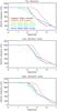 |
Fig. 8 Optimal frequencies as a function of the magnitude for conditions related to Fig. 7. |
| In the text | |
|
Fig. 9 OPD residuals as a function of magnitude, with flux variations due to 20 mas rms residual tip-tilt jitter. The OPD disturbances are 10 μm rms atmospheric OPD and 150 nm rms vibration OPD (low vibration level). The dashed lines correspond to the specification for the fringe tracker of GRAVITY, which is to stabilize the fringes below 350 nm rms on a reference star of magnitude K = 10. |
| In the text | |
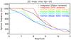 |
Fig. 10 Optimal frequencies as a function of the magnitude for conditions related to Fig. 9. |
| In the text | |
|
Fig. 11 OPD residuals as a function of magnitude with an atmospheric OPD of 15 μm rms. The vibration level is 150 nm rms per baseline (low vibration level), and the flux variations are due to 15 mas rms beam tip-tilt variations.The dashed lines correspond to the specification for the fringe tracker of GRAVITY that is to stabilize the fringes below 350 nm rms on a reference star of magnitude K = 10. |
| In the text | |
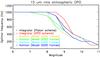 |
Fig. 12 Optimal frequencies as a function of the magnitude for conditions related to Fig. 11. |
| In the text | |
|
Fig. 13 OPD residuals as a function of magnitude for 10 μm rms atmospheric OPD, for 15 mas rms residual tip-tilt variations, and for the low vibration level (150 nm rms vibration OPD). Top: disturbance model is computed from a POL sequence acquired on the star itself (it is simply a zoom-in of Fig. 7, middle panel). Bottom: the model is computed observing a bright object (K = 7). The dashed lines correspond to the specification for the fringe tracker of GRAVITY which is to stabilize the fringes below 350 nm rms on a reference star of magnitude K = 10. |
| In the text | |
|
Fig. 14 Same as Fig. 13, except that the simulations were done for the high vibration level (240 to 380 nm rms OPD). The top panel is here a zoom-in of Fig. 7, bottom panel). |
| In the text | |
|
Fig. 15 Optimal frequencies as a function of the magnitude for conditions when the disturbance model is identified on a star of magnitude K = 7. Top panel is related to Fig. 13 and bottom panel to Fig. 14. |
| In the text | |
|
Fig. A.1 Representation of the complex visibility V and of the noise σVin the complex plane (V,ℜ,ℑ) and in the radial basis (V,V∥,V⊥). |
| In the text | |
Current usage metrics show cumulative count of Article Views (full-text article views including HTML views, PDF and ePub downloads, according to the available data) and Abstracts Views on Vision4Press platform.
Data correspond to usage on the plateform after 2015. The current usage metrics is available 48-96 hours after online publication and is updated daily on week days.
Initial download of the metrics may take a while.