| Issue |
A&A
Volume 568, August 2014
|
|
|---|---|---|
| Article Number | L1 | |
| Number of page(s) | 4 | |
| Section | Letters | |
| DOI | https://doi.org/10.1051/0004-6361/201424587 | |
| Published online | 08 August 2014 | |
Radial velocity confirmation of Kepler-91 b
Additional evidence of its planetary nature using the Calar Alto/CAFE instrument
1
Depto. de Astrofísica, Centro de Astrobiología
(CSIC-INTA), ESAC
campus,
28691 Villanueva de la Cañada
( Madrid), Spain
e-mail:
This email address is being protected from spambots. You need JavaScript enabled to view it.
2
Max Planck Institute for Astronomy, Königstuhl 17, 69117
Heidelberg,
Germany
3
Centro de Astrofísica, Universidade do Porto,
Rua das Estrelas,
4150-762
Porto,
Portugal
4
Departamento de Física e Astronomia, Faculdade de Ciências,
Universidade do Porto, 4150-762
Porto,
Portugal
5
Centro Astronómico Hispano-Alemán (CAHA), Calar Alto Observatory,
c/ Jesús Durbán Remón
2-2, 04004
Almería,
Spain
6
Instituto de Astronomía, Universidad Nacional Autonóma de México,
A.P. 70-264, 04510
México, D.F,
Mexico
Received:
11
July
2014
Accepted:
31
July
2014
Abstract
The object transiting the star Kepler-91 was recently assessed as being of planetary nature. The confirmation was achieved by analysing the light-curve modulations observed in the Kepler data. However, quasi-simultaneous studies claimed a self-luminous nature for this object, thus rejecting it as a planet. In this work, we apply anindependent approach to confirm the planetary mass of Kepler-91b by using multi-epoch high-resolution spectroscopy obtained with the Calar Alto Fiber-fed Echelle spectrograph (CAFE). We obtain the physical and orbital parameters with the radial velocity technique. In particular, we derive a value of 1.09 ± 0.20 MJup for the mass of Kepler-91b, in excellent agreement with our previous estimate that was based on the orbital brightness modulation.
Key words: planets and satellites: gaseous planets / techniques: radial velocities / planets and satellites: individual: Kepler-91 / planets and satellites: individual: KOI-2133 / planets and satellites: individual: KIC 8219268 / planet-star interactions
© ESO, 2014
1. Introduction
Several techniques, some previously applied to binary systems, have been recently improved to obtain the mass of planetary-size objects. They include radial velocity (RV) measurements (Mayor & Queloz 1995; Santerne et al. 2012), accurate astrometry (Muterspaugh et al. 2010; Lazorenko et al. 2011), microlensing (Mao & Paczynski 1991; Gould & Loeb 1992), transit-timing variations (e.g. Holman et al. 2010), or light-curve modulations (e.g. Borucki et al. 2009). Because of its easy applicability to a wide range of masses, the RV method has been the most popular in the past two decades. Currently, thanks to the unprecedented accurate photometry obtained by the Kepler telescope, several studies have confirmed the light-curve modulations produced by extrasolar planets (e.g. Borucki et al. 2009; Shporer et al. 2011; Quintana et al. 2013). The modelling of these modulations can provide the mass of the bound object, which makes it an alternative method with which to confirm its planetary nature.
Lillo-Box et al. (2014b) used this photometric
technique (together with a careful characterisation of the host star) to establish the
planetary nature of the object transiting the star Kepler-91 (KOI-2133 or KIC 8219268). It
was detected by the Kepler mission (Borucki
et al. 2011) and announced as a planet candidate in the second release of the
mission on February 2012 (Batalha et al. 2013). The
exhaustive analysis of the light-curve modulations, transit dim, and asteroseismic signals
performed by Lillo-Box et al. (2014b) led us to
classify this planet as an inflated hot Jupiter ( and
and  )
that orbits very close (
)
that orbits very close ( at periastron passage)
to a K3 III giant star (M⋆ = 1.31 ± 0.10
M⊙, R⋆ = 6.30 ± 0.16
R⊙).
at periastron passage)
to a K3 III giant star (M⋆ = 1.31 ± 0.10
M⊙, R⋆ = 6.30 ± 0.16
R⊙).
However, two studies (Esteves et al. 2013; Sliski & Kipping 2014) claimed a possible non-planetary nature for this system. Both papers suggested that it might instead be a self-luminous (and thus star-like) object. Based on transit-fitting analysis and a claimed detection of the secondary eclipse, Esteves et al. (2013) concluded that the object emits light so they rejected it as a planet. In contrast, Angerhausen et al. (2014) provided a high-level analysis of the entire light-curve (encompassing all available Kepler observations). They detected several dimmings in the phase-folded light-curve, achieved similar conclusions as Lillo-Box et al. (2014b), and suggested that the detected dimmings are poorly explained with a secondary eclipse alone. Sliski & Kipping (2014) estimated (also with transit-fitting) the mean stellar density of the star and compared it with the asteroseismic determination. The significant difference found between the two values was attributed to the non-planetary nature of the transiting object.
Therefore, the problem is still open. In this paper, we provide additional and independent confirmation of the planetary nature of Kepler-91b.
2. Observations and data analysis
2.1. Observations and basic reduction
High-resolution spectra were collected during the Kepler observing window of May−July 2012 with the Calar Alto Fiber-fed Echelle spectrograph (CAFE, Aceituno et al. 2013), mounted on the 2.2 m telescope in Calar Alto Observatory (Almería, Spain). The instrument provides an average spectral resolution of around λ/ Δλ = 63 000 across the whole spectral range between 4000 Å and 9500 Å, allowing nominal radial velocity accuracies at the level of few tens of meters per second for FGK stars.
The exposure time for Kepler-91, a mKep = 12.5 mag giant star (spectral type K3 III), was set between 1800 and 2700 s, depending on the weather conditions (seeing, atmospheric transparency, etc.). We typically obtained from two to three spectra per night for this object. The signal-to-noise ratio (S/N) was calculated as the inverse of the root mean square of the spectra over a continuum region without lines centred at 6500 Å (where the efficiency peak of CAFE is located).
In total, 40 spectra were acquired in 20 nights, with a median S/N of 11. Continuum and bias images were obtained for reduction purposes and thorium-argon (ThAr) arcs were acquired after each science spectrum to calibrate the wavelength accurately. All images were processed with the pipeline provided by the observatory (see Aceituno et al. 2013, for further details on the reduction process). It uses a specific ThAr line list of several hundred features to achieve wavelength calibration with a precision at the 1 m/s level. Every spectrum was wavelength-calibrated with the immediate arc obtained just after the science observation at the same telescope position. The data presented here were taken during the earlier periods of operations of the instrument, when the thermal and vibrational control systems were still not fully operational.
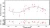 |
Fig. 1 Radial velocity data (red circles). The solid black line shows the fit to the acquired radial velocity data by assuming the period obtained by the Kepler team (Batalha et al. 2013) and the small eccentricity derived in Lillo-Box et al. (2014b) using the light-curve modulations (REB). The dotted line represents the independent curve obtained by using the parameters extracted from Lillo-Box et al. (2014b), using the REB modulations. |
2.2. Extracting the radial velocity with GAbox
We applied an active cross-correlation method to extract the radial velocity information
of the reduced spectra. Zucker (2003), it is showed
that maximum-likelihood parameter determination is equivalent to cross-correlation (see
Sect. 2 in that paper). The method assumes that the observed spectrum, f(n), can
be modelled by a template, g(n), scaled by a constant
(a0), shifted by a determined number of
bins (s0) with the addition of random white
Gaussian noise with a specific standard deviation (σ0),
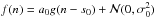 . Thus, the natural logarithm of
the likelihood function becomes
. Thus, the natural logarithm of
the likelihood function becomes ![Mathematical equation: \begin{equation} \label{eq:like} \log{L} = -N\log{\sigma_0} - \frac{1}{2\sigma_0^2} \sum_n { [f(n)-a_0g(n-s_0)]^2 } + C, \end{equation}](/articles/aa/full_html/2014/08/aa24587-14/aa24587-14-eq16.png) (1)where N is the total number of
bins (pixels) of the spectrum and C is a constant independent of the parameters. The
set of parameters
(1)where N is the total number of
bins (pixels) of the spectrum and C is a constant independent of the parameters. The
set of parameters ![Mathematical equation: \hbox{$[\hat{s}, \hat{a}, \hat{\sigma}]$}](/articles/aa/full_html/2014/08/aa24587-14/aa24587-14-eq19.png) maximising the function provides
the best fit of the modified template to the observations. In particular, ŝ can be identified with
the radial velocity of the star. This method assumes zero mean for both the template and
the observed spectrum, therefore we subtracted their corresponding means.
maximising the function provides
the best fit of the modified template to the observations. In particular, ŝ can be identified with
the radial velocity of the star. This method assumes zero mean for both the template and
the observed spectrum, therefore we subtracted their corresponding means.
We used a modified version of our genetic algorithm that we presented in Lillo-Box et al. (2014b; GAbox), to find the set of parameters maximising the likelihood in Eq. (1). We used a synthetic spectrum from Coelho et al. (2005) of the same spectral type as Kepler-91 as a template. This improved algorithm searches for the best-fit set of parameters with no need of exploring the whole parameter space (see general details of the method in Lillo-Box et al. 2014b). In this case, the routine first uses large step sizes of 5 km s-1 to search for the rough region in which the maximum is located. When this region is found, the step sizes start to decrease gradually (until the 1 m/s level) each time the algorithm finds a maximum in the likelihood function. After the final maximum has been found, the process is repeated G times, with G being the number of super-generations provided by the user (typically G> 20). The final radial velocity of a specific order (ŝ) is obtained as the median of the G convergence values. The upper and lower confidence levels of each Gi value correspond to the 3σ statistical uncertainty. The final uncertainty of the calculated RV of the order (σŝ) is computed by bootstrapping all G values with their corresponding uncertainties.
We determined one shift per order (84 in total for CAFE) and combined them to obtain the RV of the star. The final value and its uncertainty were thus computed by the median of all orders and bootstrapping the individual results to obtain 3σ errors.
Observational data and determined radial velocity. Julian date is calculated at mid-observation.
3. Results
Table 1 summarises the observing characteristics (Julian date, exposure time, S/N, and phase) as well as the RV values for each epoch obtained as explained in Sect. 2. In Fig. 1, we show the phase-folded RV data.
Prior to fitting a Keplerian orbit to the RV data, we performed a Lomb-Scargle periodogram
(Fig. 2) to check whether we detect the planetary
signal at the expected period (T
= 6.246580 ± 0.000082 days as determined by Batalha et al. 2013). We restricted the period search to a specific range.
The longest period explored was set to the longest time span between our observations (i.e.
Tmax =
tmax − tmin =
62 days, where tmax and tmin are the
earliest and latest Julian dates in our observations). Since the observations are unevenly
separated, the shortest period searched was set to the median of the inverse time interval
between data points, as was proposed by Debosscher et al.
(2007) and Ivezić et al. (2013),
 days1. The significant peak in the power spectrum
(with a false-alarm probability2 of FAP = 0.09%, over the 0.1% level) coincides
with the expected period of the planet. This provides clear confirmation for the detection
of a periodic signal. Consequently, we can affirm that we are detected the RV signal of
Kepler-91b.
days1. The significant peak in the power spectrum
(with a false-alarm probability2 of FAP = 0.09%, over the 0.1% level) coincides
with the expected period of the planet. This provides clear confirmation for the detection
of a periodic signal. Consequently, we can affirm that we are detected the RV signal of
Kepler-91b.
We then used the RVLIN software3 (Wright & Howard 2009) and its additional package
BOOTTRAN for parameter uncertainties estimation with bootstrapping (described in Wang et al. 2012) to fit our RV data to a Keplerian
orbital solution. Since we have extensive observations of its transit, the period of the
transiting object can be far more accurately determined by the transit analysis. Thus, we
decided to fix the period to that provided by Batalha et al.
(2013). Because of the relatively large uncertainties in the RV and incomplete
coverage of the RV curve, we also decided to fix the eccentricity of the orbit to the
slightly non-circular value determined by Lillo-Box et al.
(2014b),  .
The free parameters for this fitting were the semi-amplitude of the RV variations
(K), the
systemic velocity of the system (Vsys), and the orbital argument of the
periastron (ω).
.
The free parameters for this fitting were the semi-amplitude of the RV variations
(K), the
systemic velocity of the system (Vsys), and the orbital argument of the
periastron (ω).
We used the asteroseismic determination of the stellar mass of the host star by Lillo-Box et al. (2014b), M⋆ = 1.31 ± 0.1
M⊙, to obtain an accurate value of the
minimum mass of the transiting object (i.e Mpsini). Moreover, we
know that the orbit of this planet is highly inclined with respect to our line of sight. The
inclination was also provided by Lillo-Box et al.
(2014b) ( degrees) and is supported by previous light-curve analysis such as Tenenbaum et al. (2012), who derived i = 71.4 ± 2.5 degrees, in
good agreement with our value. Thus, we can directly determine the absolute mass of the
orbiting object.
degrees) and is supported by previous light-curve analysis such as Tenenbaum et al. (2012), who derived i = 71.4 ± 2.5 degrees, in
good agreement with our value. Thus, we can directly determine the absolute mass of the
orbiting object.
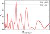 |
Fig. 2 Lomb-Scargle periodogram of the radial velocity data obtained with CAFE. The dotted lines show the false-alarm probability levels of FAP = 0.1% and FAP = 1%. The vertical dashed line shows the period derived by transit detection. The detected peak at 6.23 ± 0.03 days in this RV periodogram has an FAP = 0.09%. |
The results of the RVLIN fitting process are shown in Table 2, the fitted model is plotted in Fig. 1. We investigated the significance of that fit against a constant model (which would imply that we are just detecting noise). We infer a Bayesian information criterion (BIC4) for the constant model and for the RV model of BICconst. = 30.5 and BICRV = 27.85. This implies a ΔBIC = 2.7, which provides positive (although not strong) evidence for the RV model (positive detection) against the constant model (negative detection). Alternatively, we obtain a value of 12.7 for an F-test with weighted residuals6. This value is higher than the corresponding value of the F-distribution for a 99% confidence level, F0.01(p2 − p1, N − p2) = F0.01(3,36) = 4.38. Thus, we can confirm that the detected RV variability is significant at 99% confidence level with respect to pure noise.
Best-fit and derived parameters from the RV analysis.
The radial velocity data confirm the Jupiter-like mass (Mpsini = 1.01 ±
0.18 MJup) of the object orbiting Kepler-91.
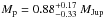
Using our previous value for the inclination, the absolute mass becomes Mp = 1.09 ± 0.20
MJup. This result agrees well, within the
uncertainties, with the derived mass in the confirmation paper of Kepler-91b (Lillo-Box et al. 2014b),
 . Moreover, the
semi-major axis aRV =
0.0726 ± 0.0019 AU also agrees extremely well with the value determined
by the light-curve modulations in Lillo-Box et al.
(2014b) of
. Moreover, the
semi-major axis aRV =
0.0726 ± 0.0019 AU also agrees extremely well with the value determined
by the light-curve modulations in Lillo-Box et al.
(2014b) of  AU. The corresponding radial velocity model using the photometrically derived parameters
obtained by Lillo-Box et al. (2014b) is also plotted
in Fig. 1 for comparison purposes.
AU. The corresponding radial velocity model using the photometrically derived parameters
obtained by Lillo-Box et al. (2014b) is also plotted
in Fig. 1 for comparison purposes.
4. Discussion and conclusions
The fit to the RV data provides orbital parameters that agree excellently well with those
obtained by the photometric analysis provided in the confirmation paper7. Thus, we present independent support of the planetary-mass of the
object transiting Kepler-91. Moreover, the transit and asteroseismic analysis yield a radius
of the transiting object of  , providing a
mean density of ρp =
0.33 ± 0.08 ρJup.
, providing a
mean density of ρp =
0.33 ± 0.08 ρJup.
These results disagree with Esteves et al. (2013) and
Sliski & Kipping (2014). The former was
already discussed in Lillo-Box et al. (2014b), where
several arguments were given against the proposed self-luminous scenario for Kepler-91b. In
brief, Esteves et al. (2013) derived a mass for the
transiting object of  and obtained
discrepant day/night-side and equilibrium temperatures based on a claimed detection of the
secondary eclipse. However, as we noted and Angerhausen
et al. (2014) concluded as well, the detection of the secondary eclipse is neither
clear nor conclusive. Moreover, given their derived mass for this companion with a
Jupiter-like radius, it is difficult to explain their proposed stellar nature. These types
of objects are only found in very young stellar associations (with ages younger than 10 Myr)
such as Collinder 69 or σ-Orionis. Thus, even assuming their derived higher
mass, this proposed false-positive configuration can be ruled out.
and obtained
discrepant day/night-side and equilibrium temperatures based on a claimed detection of the
secondary eclipse. However, as we noted and Angerhausen
et al. (2014) concluded as well, the detection of the secondary eclipse is neither
clear nor conclusive. Moreover, given their derived mass for this companion with a
Jupiter-like radius, it is difficult to explain their proposed stellar nature. These types
of objects are only found in very young stellar associations (with ages younger than 10 Myr)
such as Collinder 69 or σ-Orionis. Thus, even assuming their derived higher
mass, this proposed false-positive configuration can be ruled out.
The alternative explanation provided by Esteves et al. (2013) suggests that the system is actually an eclipsing binary diluted by a contaminating third stellar source, a foreground or background star. However, Lillo-Box et al. (2012, 2014a) provided high-resolution images of this system (among other Kepler candidates) to rule out this and other configurations. According to Sect. 4.1.2 of the latter paper (based on Law et al. 2013), the planetary transit of Kepler-91b cannot be mimicked by the presence of a diluted star fainter than the transited star. Only a blended source with a very small radius that is brighter than the transited star can dilute the binary eclipse and mimic a planetary transit. However, in the high-resolution image obtained by Lillo-Box et al. (2014a) we did not find companions farther away than 0.1 arcsec. Thus, the probability for an undetected chance-aligned source brighter than 12.5 magnitudes and closer than 0.1 arcsec is lower than 10-6.
Sharing the opinion of Esteves et al. (2013), Sliski & Kipping (2014) also classified
Kepler-91b as a false positive. They compared the asteroseismic determination of the stellar
density ρ⋆,astero = 6.81 ± 0.32
kg / m3 (derived by Huber et al. 2013) with the observed value
 derived by them
directly from transit fitting. Based on the large discrepancy between the two values, they
concluded that to explain this disagreement, the orbit of the planet would have to be highly
eccentric such that the planet is essentially expected to be in-contact with the star.
Basically, their derived observed stellar density corresponds to a semi-major axis of the
companion of
derived by them
directly from transit fitting. Based on the large discrepancy between the two values, they
concluded that to explain this disagreement, the orbit of the planet would have to be highly
eccentric such that the planet is essentially expected to be in-contact with the star.
Basically, their derived observed stellar density corresponds to a semi-major axis of the
companion of  ,
similar to that of Esteves et al. (2013),
a/R⋆ =
4.5. The authors claimed that the two determinations of the semi-major
axis are independent, but they both used the same set of photometric data and the same
observational effect (the transit signal).
,
similar to that of Esteves et al. (2013),
a/R⋆ =
4.5. The authors claimed that the two determinations of the semi-major
axis are independent, but they both used the same set of photometric data and the same
observational effect (the transit signal).
Instead, we have determined the semi-major axis of the orbit by using three truly
independent observational effects, namely the transit fitting (a/R⋆)transit
= 2.40 ± 0.12 (also supported by the previous analysis of Tenenbaum et al. 2012), light-curve modulations in the
out-of-transit region ( ,
and the current radial velocity analysis (a/R⋆)RV
= 2.48 ± 0.12. All three estimations provide autonomous and coincident
measurements of the semi-major axis. As stated by Sliski
& Kipping (2014) and already pointed out in Lillo-Box et al. (2014b), this lower value implies an observed stellar density
that agrees excellently with the asteroseismic analysis, thus confirming the planetary
nature of the object orbiting Kepler-91 and rejecting the self-luminous scenario. Possible
explanations for the large discrepancy of the other determinations of a/R⋆
might involve some assumptions when fitting the transit. They both assumed i) a circular
orbit, while we found that the shape of the ellipsoidal variations need a non-zero
− although low- eccentricity;
and ii) a spherical shape for the host star, which does not apply here since we clearly find
light-curve modulations due to deformations of the stellar atmosphere.
,
and the current radial velocity analysis (a/R⋆)RV
= 2.48 ± 0.12. All three estimations provide autonomous and coincident
measurements of the semi-major axis. As stated by Sliski
& Kipping (2014) and already pointed out in Lillo-Box et al. (2014b), this lower value implies an observed stellar density
that agrees excellently with the asteroseismic analysis, thus confirming the planetary
nature of the object orbiting Kepler-91 and rejecting the self-luminous scenario. Possible
explanations for the large discrepancy of the other determinations of a/R⋆
might involve some assumptions when fitting the transit. They both assumed i) a circular
orbit, while we found that the shape of the ellipsoidal variations need a non-zero
− although low- eccentricity;
and ii) a spherical shape for the host star, which does not apply here since we clearly find
light-curve modulations due to deformations of the stellar atmosphere.
The results presented here, together with the original confirmation paper (Lillo-Box et al. 2014b), provide strong evidence for the planetary-nature of Kepler-91b. Finally, this is the first planet confirmed from CAHA using CAFE, and we have proved the capability of this instrument for this type of research.
Eyer & Bartholdi (1999) claimed that for most practical cases, lower periodicities (higher frequencies) can be detected even for strongly (but randomly) under-sampled observations.
Calculated by using the astroML python module (Vanderplas et al. 2012) and its bootstrapping package.
BIC = χ2 +
klog N, where
 ,
k is the
number of free parameters, and N is the number of data points.
,
k is the
number of free parameters, and N is the number of data points.
Assuming a circular orbit, we obtain BICRV(e = 0) = 28.3.
 ,
where p1 and p2 are the free
parameters of both models (so that p2>p1),
and N the
number of data points.
,
where p1 and p2 are the free
parameters of both models (so that p2>p1),
and N the
number of data points.
The agreement between the ellipsoidal modulation mass and the RV mass has already been demonstrated in systems such TrES-2 or HAT-P-7 (see Faigler & Mazeh 2014).
Acknowledgments
This research has been funded by Spanish grant AYA2012-38897-C02-01. J.L.-B. thanks the CSIC JAE-predoc programme for the Ph.D. fellowship. We also thank CAHA for allocating our observing runs. P.F. and N.C.S. acknowledge support by Fundação para a Ciência e a Tecnologia (FCT) through Investigador FCT contracts of reference IF/01037/2013 and IF/00169/2012, respectively, and POPH/FSE (EC) by FEDER funding through the program “Programa Operacional de Factores de Competitividade − COMPETE”. We also acknowledge the support from the European Research Council/European Community under the FP7 through Starting Grant agreement number 239953.
References
- Aceituno, J., Sánchez, S. F., Grupp, F., et al. 2013, A&A, 552, A31 [NASA ADS] [CrossRef] [EDP Sciences] [Google Scholar]
- Angerhausen, D., DeLarme, E., & Morse, J. A. 2014, ApJ, submitted [arXiv:1404.4348] [Google Scholar]
- Batalha, N. M., Rowe, J. F., Bryson, S. T., et al. 2013, ApJS, 204, 24 [NASA ADS] [CrossRef] [Google Scholar]
- Borucki, W. J., Koch, D., Jenkins, J., et al. 2009, Science, 325, 709 [NASA ADS] [CrossRef] [PubMed] [Google Scholar]
- Borucki, W. J., Koch, D. G., Basri, G., et al. 2011, ApJ, 736, 19 [NASA ADS] [CrossRef] [Google Scholar]
- Coelho, P., Barbuy, B., Meléndez, J., Schiavon, R. P., & Castilho, B. V. 2005, A&A, 443, 735 [NASA ADS] [CrossRef] [EDP Sciences] [Google Scholar]
- Debosscher, J., Sarro, L. M., Aerts, C., et al. 2007, A&A, 475, 1159 [NASA ADS] [CrossRef] [EDP Sciences] [Google Scholar]
- Esteves, L. J., De Mooij, E. J. W., & Jayawardhana, R. 2013, ApJ, 772, 51 [NASA ADS] [CrossRef] [Google Scholar]
- Eyer, L., & Bartholdi, P. 1999, A&AS, 135, 1 [NASA ADS] [CrossRef] [EDP Sciences] [Google Scholar]
- Faigler, S., & Mazeh, T. 2014, ApJ, submitted [arXiv:1407.2361] [Google Scholar]
- Gould, A., & Loeb, A. 1992, ApJ, 396, 104 [NASA ADS] [CrossRef] [Google Scholar]
- Holman, M. J., Fabrycky, D. C., Ragozzine, D., et al. 2010, Science, 330, 51 [NASA ADS] [CrossRef] [PubMed] [Google Scholar]
- Huber, D., Chaplin, W. J., Christensen-Dalsgaard, J., et al. 2013, ApJ, 767, 127 [NASA ADS] [CrossRef] [Google Scholar]
- Ivezić, Ż., Connolly, A., VanderPlas, J., & Gray, A. 2013, Statistics, Data Mining, and Machine Learning in Astronomy (Princeton University Press) [Google Scholar]
- Law, N. M., Morton, T., Baranec, C., et al. 2013, ApJ, submitted [arXiv:1312.4958] [Google Scholar]
- Lazorenko, P. F., Sahlmann, J., Ségransan, D., et al. 2011, A&A, 527, A25 [NASA ADS] [CrossRef] [EDP Sciences] [Google Scholar]
- Lillo-Box, J., Barrado, D., & Bouy, H. 2012, A&A, 546, A10 [NASA ADS] [CrossRef] [EDP Sciences] [Google Scholar]
- Lillo-Box, J., Barrado, D., & Bouy, H. 2014a, A&A, 566, A103 [NASA ADS] [CrossRef] [EDP Sciences] [Google Scholar]
- Lillo-Box, J., Barrado, D., Moya, A., et al. 2014b, A&A, 562, A109 [NASA ADS] [CrossRef] [EDP Sciences] [Google Scholar]
- Mao, S., & Paczynski, B. 1991, ApJ, 374, L37 [NASA ADS] [CrossRef] [Google Scholar]
- Mayor, M., & Queloz, D. 1995, Nature, 378, 355 [NASA ADS] [CrossRef] [Google Scholar]
- Muterspaugh, M. W., Lane, B. F., Kulkarni, S. R., et al. 2010, AJ, 140, 1657 [NASA ADS] [CrossRef] [Google Scholar]
- Quintana, E. V., Rowe, J. F., Barclay, T., et al. 2013, ApJ, 767, 137 [NASA ADS] [CrossRef] [Google Scholar]
- Santerne, A., Díaz, R. F., Moutou, C., et al. 2012, A&A, 545, A76 [NASA ADS] [CrossRef] [EDP Sciences] [Google Scholar]
- Shporer, A., Jenkins, J. M., Rowe, J. F., et al. 2011, AJ, 142, 195 [NASA ADS] [CrossRef] [Google Scholar]
- Sliski, D. H., & Kipping, D. M. 2014, ApJ, accepted [arXiv:1401.1207] [Google Scholar]
- Tenenbaum, P., Jenkins, J. M., Seader, S., et al. 2012, ApJS, submitted [arXiv:1212.2915] [Google Scholar]
- Vanderplas, J., Connolly, A., Ivezić, Ž., & Gray, A. 2012, in Conf. on Intelligent Data Understanding (CIDU), 47 [Google Scholar]
- Wang, S. X., Wright, J. T., Cochran, W., et al. 2012, ApJ, 761, 46 [NASA ADS] [CrossRef] [Google Scholar]
- Wright, J. T., & Howard, A. W. 2009, ApJS, 182, 205 [NASA ADS] [CrossRef] [Google Scholar]
- Zucker, S. 2003, MNRAS, 342, 1291 [Google Scholar]
All Tables
Observational data and determined radial velocity. Julian date is calculated at mid-observation.
All Figures
|
Fig. 1 Radial velocity data (red circles). The solid black line shows the fit to the acquired radial velocity data by assuming the period obtained by the Kepler team (Batalha et al. 2013) and the small eccentricity derived in Lillo-Box et al. (2014b) using the light-curve modulations (REB). The dotted line represents the independent curve obtained by using the parameters extracted from Lillo-Box et al. (2014b), using the REB modulations. |
| In the text | |
|
Fig. 2 Lomb-Scargle periodogram of the radial velocity data obtained with CAFE. The dotted lines show the false-alarm probability levels of FAP = 0.1% and FAP = 1%. The vertical dashed line shows the period derived by transit detection. The detected peak at 6.23 ± 0.03 days in this RV periodogram has an FAP = 0.09%. |
| In the text | |
Current usage metrics show cumulative count of Article Views (full-text article views including HTML views, PDF and ePub downloads, according to the available data) and Abstracts Views on Vision4Press platform.
Data correspond to usage on the plateform after 2015. The current usage metrics is available 48-96 hours after online publication and is updated daily on week days.
Initial download of the metrics may take a while.