© ESO, 2014

1. Introduction

Strong gravitational lensing by galaxies is a powerful tool for cosmological studies, in particular regarding precise mass estimates of the inner region of galaxies, the angular structure of the mass distribution (e.g., ellipticity and orientation), and mass substructure (see, e.g., Kochanek 2006; Treu 2010; Bartelmann 2010, and references therein). In his pioneering paper, Refsdal (1964) pointed out the possibility of determining cosmological parameters from lensing, specifically the Hubble constant, from measurements of time delays in lens systems. Whereas time delays have been determined in some 20 lens systems by now, the accuracy of the corresponding values of H₀ is difficult to judge, because of the difficulty of reliably constraining the mass distribution of the lens: on the one hand, the number of observational constraints can be insufficient to constrain the mass distribution to sufficient accuracy. On the other hand, Falco et al. (1985) have found that there exists a transformation of the mass distribution of the lens that leaves all observables invariant, except for the product of time delay and H₀. Thus, although very detailed studies of some lens systems have been conducted (see, e.g., Suyu et al. 2013), this mass-sheet transformation (MST) poses a fundamental limitation of the accuracy of the derived value for H₀ from gravitational lensing alone. Although the degeneracy caused by the MST can be broken with additional observations, such as stellar dynamics in the lens or some additional information about the properties of the source (such as its luminosity), the current accuracy on these quantities leads to uncertainties of H₀ larger than those from other methods, and the method may be biased. In practice, the degeneracy due to the MST is broken by assumptions about the mass distribution, e.g., that it follows a power law. A recent discussion of the impact of the MST on H₀ determination can be found in Schneider & Sluse (2013).

A different approach to cosmology by strong-lens systems involves the relative lensing strength for two sources at two different redshifts. It is known that the classical MST is an exact transformation of the lens mass distribution only for sources at a single distance, and that it can be broken in principle when sources at several redshifts are employed (Bradač et al. 2004). However, it must be stressed that this degeneracy-breaking assumes that there is no second deflector along the line of sight to the sources. In reality, the lower-redshift sources have masses and consequently act as additional lenses for higher-redshift sources.

The recent discovery of a strong galaxy-scale lens with two extended multiple-image arc structures from two sources at vastly different redshifts (SDSSJ0946+1006; Gavazzi et al. 2008) opened up the possibility of studying a multi-plane lens system in great detail. Collett & Auger (2014; hereafter CA14) performed a detailed analysis of this system by constructing a model that involves both the main lens in the foreground of the two sources, and a smaller-mass deflector associated with the lower-redshift source. The relative lens strength β of the main lens on the two sources depends on distance ratios, which in turn depend on the redshifts of lenses and sources involved as well as on the distance-redshift relation in the Universe. Since the latter is sensitive to the density parameters and the equation of state parameter w of dark energy, CA14 were able to obtain constraints on w from this lens system.

In this Letter, we investigate whether this method can yield reliable results. Specifically, we show in Sect.2 that an analog of the MST also exists for the case of two lens and two source planes, as is the case for SDSSJ0946+1006. We then demonstrate in Sect.3 that a change of cosmological parameters that leads to a change of the expected value of β is equivalent to such a generalized MST. We then study the amplitude of this equivalent MST for a range of values of w, concluding that the transformation amplitude across a plausible range of w is indeed very small. Since the MST leads to a shape of the transformed density profile that is different from the original, we conclude that this method heavily relies on assumptions made for the shape of the mass profiles of the lenses.

2. Mass-sheet transformation for two lens planes

In this section we first summarize the lensing equations for the multi-plane case (Sect.2.1), specify our notation, and recall the MST in the single-plane case (Sect.2.2) before we derive the new MST for two lens and two source planes.

2.1. Multi-plane lens equations

We consider lenses and sources distributed along nearly the same line of sight at N different distances from us, characterized by their redshifts z_i, or angular-diameter distances D_i from us, 1 ≤ i ≤ N (we largely follow the notation of Schneider et al. 1992, where more details of the derivation are given). Perpendicular to the line of sight, we consider planes in which the sources at these distances are located, and onto which the mass distribution of the deflecting masses are projected (lens/source planes). We denote by D_ij the angular-diameter distance of the jth plane as seen from the i-th plane, with 1 ≤ i<j ≤ N. The projected mass distribution in the i-th plane is characterized by its surface mass density Σ_i(ξ) and gives rise to a deflection angle 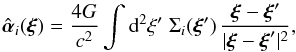${\hat{{\alpha }}}_{\mathit{i}}\mathrm{\left(}{{\xi }}_{\mathit{i}}\mathrm{\right)}$, where ${\hat{{\alpha }}}_{\mathit{i}}\mathrm{\left(}{\xi }\mathrm{\right)}\mathrm{=}\frac{\mathrm{4}\mathit{G}}{{\mathit{c}}^{\mathrm{2}}}\mathrm{\int }{\mathrm{d}}^{\mathrm{2}}{\mathit{\xi }}^{\mathrm{\prime }}{\mathrm{\Sigma }}_{\mathit{i}}\mathrm{\left(}{{\xi }}^{\mathrm{\prime }}\mathrm{\right)}\hspace{0.17em}\frac{{\xi }\mathrm{-}{{\xi }}^{\mathrm{\prime }}}{\mathrm{|}{\xi }\mathrm{-}{{\xi }}^{\mathrm{\prime }}{\mathrm{|}}^{\mathrm{2}}}\mathit{,}$(1)and ξ_i = D_iθ_i is a transverse separation vector in the ith plane, with the corresponding unlensed angular position θ_i. The resulting propagation equations of a light ray follows solely from geometry and the definition of angular-diameter distances, 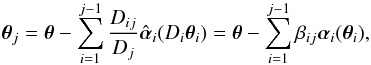${{\theta }}_{\mathit{j}}\mathrm{=}{\theta }\mathrm{-}\sum _{\mathit{i}\mathrm{=}\mathrm{1}}^{\mathit{j}\mathrm{-}\mathrm{1}}\frac{{\mathit{D}}_{\mathit{ij}}}{{\mathit{D}}_{\mathit{j}}}\hat{{\alpha }}\mathit{i}\mathrm{\left(}{\mathit{D}}_{\mathit{i}}{{\theta }}_{\mathit{i}}\mathrm{\right)}\mathrm{=}{\theta }\mathrm{-}\sum _{\mathit{i}\mathrm{=}\mathrm{1}}^{\mathit{j}\mathrm{-}\mathrm{1}}{\mathit{\beta }}_{\mathit{ij}}{{\alpha }}_{\mathit{i}}\mathrm{\left(}{{\theta }}_{\mathit{i}}\mathrm{\right)}\mathit{,}$(2)where we set θ ≡ θ₁, scaled the deflection angles $\hat{{\alpha }}{}_{\mathit{i}}$ to the final source plane at i = N, i.e., 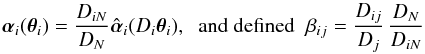${{\alpha }}_{\mathit{i}}\mathrm{\left(}{{\theta }}_{\mathit{i}}\mathrm{\right)}\mathrm{=}\frac{{\mathit{D}}_{\mathit{iN}}}{{\mathit{D}}_{\mathit{N}}}\hat{{\alpha }}\mathit{i}\mathrm{\left(}{\mathit{D}}_{\mathit{i}}{{\theta }}_{\mathit{i}}\mathrm{\right)}\mathit{,}\mathrm{anddefined}{\mathit{\beta }}_{\mathit{ij}}\mathrm{=}\frac{{\mathit{D}}_{\mathit{ij}}}{{\mathit{D}}_{\mathit{j}}}\hspace{0.17em}\frac{{\mathit{D}}_{\mathit{N}}}{{\mathit{D}}_{\mathit{iN}}}$(3)as coefficients of relative distance ratios. Accordingly, we define the dimensionless surface mass densities κ_i(θ_i) = 4πGD_iD_iN Σ_i(D_iθ_i)/(c²D_N), which satisfy ∇·α_i = 2κ_i.

2.2. Summary of the single-plane MST

We briefly recall the MST for the single-lens plane, for which N = 2 (see Falco et al. 1985; Schneider & Sluse 2013, and references therein). Hence, we have a single lens plane at redshift z₁ with deflection α(θ) ≡ α₁(θ₁) and dimensionless surface mass density κ(θ) ≡ κ₁(θ₁), and a single source plane at redshift z₂.

If a mass distribution κ(θ) can explain all the observed lensing features, such as image positions, flux ratios, relative image shapes, and time-delay ratios, of a source with unlensed brightness profile I^s(θ₂), then the whole family of mass distributions and corresponding scaled deflection angles ${\mathit{\kappa }}_{\mathit{\lambda }}\mathrm{\left(}{\theta }\mathrm{\right)}\mathrm{=}\mathit{\lambda \kappa }\mathrm{\left(}{\theta }\mathrm{\right)}\mathrm{+}\mathrm{(}\mathrm{1}\mathrm{-}\mathit{\lambda }\mathrm{)}\mathrm{;} {{\alpha }}_{\mathit{\lambda }}\mathrm{\left(}{\theta }\mathrm{\right)}\mathrm{=}\mathit{\lambda }{\alpha }\mathrm{\left(}{\theta }\mathrm{\right)}\mathrm{+}\mathrm{(}\mathrm{1}\mathrm{-}\mathit{\lambda }\mathrm{)}{\theta }$(4)explains the lensed features equally well for a source of brighness profile ${\mathit{I}}_{\mathit{\lambda }}^{\mathrm{s}}\mathrm{\left(}{{\theta }}_{\mathrm{2}}\mathrm{\right)}\mathrm{=}{\mathit{I}}^{\mathrm{s}}\mathrm{(}{{\theta }}_{\mathrm{2}}\mathit{/}\mathit{\lambda }\mathrm{)}$. Hence, the transformed brightness distribution in the source plane is rescaled by a factor λ. This rescaling of the source plane implies that the magnification of images is changed, μ_λ = μ/λ², but that can only be observed if the luminosity or physical size of the source is known (standard candle or standard rod). In most cases, this information is unavailable, so that the magnification cannot be obtained from observations, whereas magnification (and thus flux) ratios are invariant under the MST. The time delay between pairs of images is changed under the MST, so that a time delay measurement can be employed to break the degeneracy caused by the MST, provided the Hubble constant (and the density parameters of our Universe) are assumed to be known.

2.3. MST for two source and lens planes

We now study whether a similar invariance transformation exists for sources at two different redshifts z₂ and z₃, with lenses at redshift z₁ and z₂. In particular, we consider that the closer source at z₂ is associated with mass that deflects light rays from the more distant source. By specializing the equations of Sect.2.1 to the case N = 3, we obtain the pair of relations ${{\theta }}_{\mathrm{2}}\mathrm{=}{\theta }\mathrm{-}\mathit{\beta }\hspace{0.17em}{{\alpha }}_{\mathrm{1}}\mathrm{\left(}{\theta }\mathrm{\right)}\mathrm{;}{{\theta }}_{\mathrm{3}}\mathrm{=}{\theta }\mathrm{-}{{\alpha }}_{\mathrm{1}}\mathrm{\left(}{\theta }\mathrm{\right)}\mathrm{-}{{\alpha }}_{\mathrm{2}}\mathrm{\left(}{{\theta }}_{\mathrm{2}}\mathrm{\right)}\mathit{,}$(5)where we defined β ≡ β₁₂ (see Eq. (3)). A mass-sheet transformation is defined as a change of the deflection angles (and correspondingly the lensing mass distributions) such that the lens equations remain invariant, with only a uniform isotropic scaling in the source planes. Considering the first of Eq. (5), a MST for the first source plane is obtained by applying the single-lens plane MST to the effective deflection βα₁, i.e., by setting (here and in the following, a prime denotes transformed quantities) 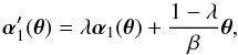${{\alpha }}_{\mathrm{1}}^{\mathrm{\prime }}\mathrm{\left(}{\theta }\mathrm{\right)}\mathrm{=}\mathit{\lambda }{{\alpha }}_{\mathrm{1}}\mathrm{\left(}{\theta }\mathrm{\right)}\mathrm{+}\frac{\mathrm{1}\mathrm{-}\mathit{\lambda }}{\mathit{\beta }}{\theta }\mathit{,}$(6)after which the transformed position at z₂ becomes 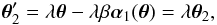${{\theta }}_{\mathrm{2}}^{\mathrm{\prime }}\mathrm{=}\mathit{\lambda }{\theta }\mathrm{-}\mathit{\lambda \beta }{{\alpha }}_{\mathrm{1}}\mathrm{\left(}{\theta }\mathrm{\right)}\mathrm{=}\mathit{\lambda }{{\theta }}_{\mathrm{2}}\mathit{,}$(7)i.e., the required uniform isotropic scaling. The question now is whether we can find a transformation of the deflection angle α₂ such that the second of Eq. (5) also remains invariant up to a scaling of θ₃. If ${{\alpha }}_{\mathrm{2}}^{\mathrm{\prime }}\mathrm{\left(}{{\theta }}_{\mathrm{2}}^{\mathrm{\prime }}\mathrm{\right)}$ denotes the transformed deflection angle, then the transformed lens equation reads 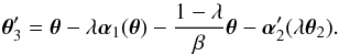${{\theta }}_{\mathrm{3}}^{\mathrm{\prime }}\mathrm{=}{\theta }\mathrm{-}\mathit{\lambda }{{\alpha }}_{\mathrm{1}}\mathrm{\left(}{\theta }\mathrm{\right)}\mathrm{-}\frac{\mathrm{1}\mathrm{-}\mathit{\lambda }}{\mathit{\beta }}{\theta }\mathrm{-}{{\alpha }}_{\mathrm{2}}^{\mathrm{\prime }}\mathrm{\left(}\mathit{\lambda }{{\theta }}_{\mathrm{2}}\mathrm{\right)}\mathit{.}$(8)Requiring that ${{\theta }}_{\mathrm{3}}^{\mathrm{\prime }}\mathrm{=}{\mathit{\nu }}_{\mathrm{3}}{{\theta }}_{\mathrm{3}}$, corresponding to uniform scaling with the factor ν₃, we obtain 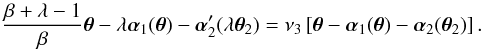$\frac{\mathit{\beta }\mathrm{+}\mathit{\lambda }\mathrm{-}\mathrm{1}}{\mathit{\beta }}{\theta }\mathrm{-}\mathit{\lambda }{{\alpha }}_{\mathrm{1}}\mathrm{\left(}{\theta }\mathrm{\right)}\mathrm{-}{{\alpha }}_{\mathrm{2}}^{\mathrm{\prime }}\mathrm{\left(}\mathit{\lambda }{{\theta }}_{\mathrm{2}}\mathrm{\right)}\mathrm{=}{\mathit{\nu }}_{\mathrm{3}}\left[{\theta }\mathrm{-}{{\alpha }}_{\mathrm{1}}\mathrm{\left(}{\theta }\mathrm{\right)}\mathrm{-}{{\alpha }}_{\mathrm{2}}\mathrm{\left(}{{\theta }}_{\mathrm{2}}\mathrm{\right)}\right]\mathit{.}$(9)To satisfy this equation, the term ${{\alpha }}_{\mathrm{2}}^{\mathrm{\prime }}$ on the l.h.s. of Eq. (9) must contain the term ν₃α₂(θ₂). Therefore, we set ${{\alpha }}_{\mathrm{2}}^{\mathrm{\prime }}\mathrm{\left(}{{\theta }}_{\mathrm{2}}^{\mathrm{\prime }}\mathrm{\right)}\mathrm{=}{\mathit{\nu }}_{\mathrm{3}}{{\alpha }}_{\mathrm{2}}\mathrm{(}{{\theta }}_{\mathrm{2}}^{\mathrm{\prime }}\mathit{/}\mathit{\lambda }\mathrm{)}\mathrm{+}{\mathit{K}}_{\mathrm{2}}{{\theta }}_{\mathrm{2}}^{\mathrm{\prime }}\mathrm{=}{\mathit{\nu }}_{\mathrm{3}}{{\alpha }}_{\mathrm{2}}\mathrm{(}{{\theta }}_{\mathrm{2}}^{\mathrm{\prime }}\mathit{/}\mathit{\lambda }\mathrm{)}\mathrm{+}{\mathit{K}}_{\mathrm{2}}\mathit{\lambda }\left[{\theta }\mathrm{-}\mathit{\beta }{{\alpha }}_{\mathrm{1}}\mathrm{\left(}{\theta }\mathrm{\right)}\right]\mathit{,}$(10)where in the second step we used ${{\theta }}_{\mathrm{2}}^{\mathrm{\prime }}\mathrm{=}\mathit{\lambda }{{\theta }}_{\mathrm{2}}$ and the first of Eq. (5). Here, K₂ is a constant, to be constrained later. Inserting Eq. (10) into Eq. (9), we see that the terms involving α₂ vanish. Comparing the remaining terms proportional to α₁ and θ, we find the pair of constraints λ − K₂λβ = ν₃ and β + λ − 1 − K₂λβ = βν₃, which have the unique solution 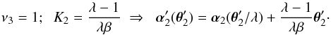${\mathit{\nu }}_{\mathrm{3}}\mathrm{=}\mathrm{1}\mathrm{;}{\mathit{K}}_{\mathrm{2}}\mathrm{=}\frac{\mathit{\lambda }\mathrm{-}\mathrm{1}}{\mathit{\lambda \beta }}\mathrm{\Rightarrow }{{\alpha }}_{\mathrm{2}}^{\mathrm{\prime }}\mathrm{\left(}{{\theta }}_{\mathrm{2}}^{\mathrm{\prime }}\mathrm{\right)}\mathrm{=}{{\alpha }}_{\mathrm{2}}\mathrm{(}{{\theta }}_{\mathrm{2}}^{\mathrm{\prime }}\mathit{/}\mathit{\lambda }\mathrm{)}\mathrm{+}\frac{\mathit{\lambda }\mathrm{-}\mathrm{1}}{\mathit{\lambda \beta }}{{\theta }}_{\mathrm{2}}^{\mathrm{\prime }}\mathrm{·}$(11)Hence we obtain a solution of Eq. (9) and accordingly a transformation of the mass distributions in both lens planes, which leads to at most a uniform isotropic scaling of the source planes.

The transformation of the first lens plane is a normal MST, in that the deflection angle (and thus the surface mass density) is scaled by an overall factor λ, and a uniform density K₁ = (1 − λ) /β is added, leading to a scaling of the first source plane by a factor λ. This scaling equally applies to the light distribution and the mass distribution, as seen by Eq. (10). Thus, after the MST, both the light and the mass in the plane i = 2 are transformed in exactly the same way. In particular, this means that if the original model has a mass component centered on a light component, the same remains true after the MST, but both are located at a position that differs by a factor of λ.

Condition (10) furthermore implies that the transformed deflection in the second lens plane is a scaled version of the original deflection, plus a contribution from a uniform mass sheet K₂. The implication of the scaling of the first term in Eq. (10) on the corresponding mass distribution can be seen as follows: if 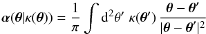${\alpha }\mathrm{\left(}{\theta }\mathrm{\right|}\mathit{\kappa }\mathrm{\left(}{\theta }\mathrm{\right)}\mathrm{)}\mathrm{=}\frac{\mathrm{1}}{\mathit{\pi }}\mathrm{\int }{\mathrm{d}}^{\mathrm{2}}{\mathit{\theta }}^{\mathrm{\prime }}\mathit{\kappa }\mathrm{(}{{\theta }}^{\mathrm{\prime }}\mathrm{)}\hspace{0.17em}\frac{{\theta }\mathrm{-}{{\theta }}^{\mathrm{\prime }}}{\mathrm{|}{\theta }\mathrm{-}{{\theta }}^{\mathrm{\prime }}{\mathrm{|}}^{\mathrm{2}}}$(12)is the deflection caused by the mass distribution κ, then 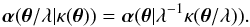${\alpha }\mathrm{(}{\theta }\mathit{/}\mathit{\lambda }\mathrm{|}\mathit{\kappa }\mathrm{\left(}{\theta }\mathrm{\right)}\mathrm{)}\mathrm{=}{\alpha }\mathrm{(}{\theta }\mathrm{\left|}{\mathit{\lambda }}^{-1}\mathit{\kappa }\mathrm{\right(}{\theta }\mathit{/}\mathit{\lambda }\mathrm{\left)}\mathrm{\right)}\mathit{.}$(13)Hence, the transformed mass distribution ${\mathit{\kappa }}_{\mathrm{2}}^{\mathrm{\prime }}$ is a scaled version of the original one, multiplied by a factor λ^-1, plus a uniform mass sheet. It must be stressed here that the phrase “adding a uniform mass sheet” corresponds to a global interpretation of the MST; however, only a relatively small inner region of the lens is probed by strong lensing, and hence the MST needs to apply only locally. Its main effect is the change of the local slope of the mass profile near the Einstein radius of a lens, making it flatter (steeper) for λ< 1 (λ> 1). The global interpretation of the mass sheet as an “external convergence”, relating it to the large-scale environment of the lens which can be probed by the observed density field of galaxies (e.g., Wong et al. 2011; Collett et al. 2013; Greene et al. 2013), constitutes an extrapolation over a vast range of scales.

Surprisingly, the second source plane remains unscaled under this MST, because of ν₃ = 1. Hence, the MST implies no change in the mapping of the second source plane, including no change in the magnification matrix. Whereas simple algebra has straightforwardly led to this result, the geometrical reason for this appears unclear.

If the MST is such that the scaling in the first lens plane corresponds to an additional focusing, which means λ< 1, so that the uniform mass sheet has positive convergence, then the mass sheet in the second lens plane has negative convergence, since the sign of K₂ is opposite to that of 1 − λ. In particular, λ = 1 implies K₂ = 0, so there is no MST that leaves the first lens plane invariant and only affects the second one. It must be stressed that the MST leaves the global lens mapping invariant and thus applies to sources of (in principle) arbitrary extent. This is quite different from other modifications of the lens mass distribution (e.g., Coe et al. 2008; Liesenborgs et al. 2008; Liesenborgs & De Rijcke 2012, and references therein), which apply to a discrete set of isolated small images of sources.

2.4. Time delay

We now consider the impact of the MST on the time delay. For sources at z₂, the MST is a normal single-plane MST, and the time delays are changed by a factor λ. For sources at z₃, we use the expression for the light travel-time from θ₃ via θ₂ and θ to the observer, as given in Schneider et al. (1992), 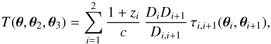$\mathit{T}\mathrm{\left(}{\theta }\mathit{,}{{\theta }}_{\mathrm{2}}\mathit{,}{{\theta }}_{\mathrm{3}}\mathrm{\right)}\mathrm{=}\sum _{\mathit{i}\mathrm{=}\mathrm{1}}^{\mathrm{2}}\frac{\mathrm{1}\mathrm{+}{\mathit{z}}_{\mathit{i}}}{\mathit{c}}\hspace{0.17em}\frac{{\mathit{D}}_{\mathit{i}}{\mathit{D}}_{\mathit{i}\mathrm{+}\mathrm{1}}}{{\mathit{D}}_{\mathit{i,i}\mathrm{+}\mathrm{1}}}\hspace{0.17em}{\mathit{\tau }}_{\mathit{i,i}\mathrm{+}\mathrm{1}}\mathrm{\left(}{{\theta }}_{\mathit{i}}\mathit{,}{{\theta }}_{\mathit{i}\mathrm{+}\mathrm{1}}\mathrm{\right)}\mathit{,}$(14)where τ_{i,i + 1} = (θ_i − θ_{i + 1})²/ 2 − β_{i,i + 1}ψ_i(θ_i) is the Fermat potential corresponding to neighboring planes, with β₁₂ ≡ β and β₂₃ = 1, and ψ_i(θ_i) is the deflection potential with ∇ψ_i = α_i. We now consider how T behaves under an MST. The scalings (6) and (10) of α_i imply that 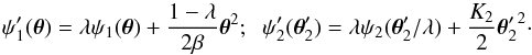${\mathit{\psi }}_{\mathrm{1}}^{\mathrm{\prime }}\mathrm{\left(}{\theta }\mathrm{\right)}\mathrm{=}\mathit{\lambda }{\mathit{\psi }}_{\mathrm{1}}\mathrm{\left(}{\theta }\mathrm{\right)}\mathrm{+}\frac{\mathrm{1}\mathrm{-}\mathit{\lambda }}{\mathrm{2}\mathit{\beta }}{{\theta }}^{\mathrm{2}}\mathrm{;}{\mathit{\psi }}_{\mathrm{2}}^{\mathrm{\prime }}\mathrm{\left(}{{\theta }}_{\mathrm{2}}^{\mathrm{\prime }}\mathrm{\right)}\mathrm{=}\mathit{\lambda }{\mathit{\psi }}_{\mathrm{2}}\mathrm{(}{{\theta }}_{\mathrm{2}}^{\mathrm{\prime }}\mathit{/}\mathit{\lambda }\mathrm{)}\mathrm{+}\frac{{\mathit{K}}_{\mathrm{2}}}{\mathrm{2}}{{{\theta }}_{\mathrm{2}}^{\mathrm{\prime }}}^{\mathrm{2}}\mathrm{·}$(15)Together with ${{\theta }}_{\mathrm{2}}^{\mathrm{\prime }}\mathrm{=}\mathit{\lambda }{{\theta }}_{\mathrm{2}}$ and ${{\theta }}_{\mathrm{3}}^{\mathrm{\prime }}\mathrm{=}{{\theta }}_{\mathrm{3}}$, we obtain 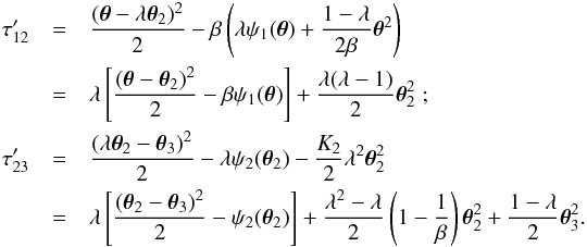$\begin{array}{ccc}{\mathit{\tau }}_{\mathrm{12}}^{\mathrm{\prime }}& \mathrm{=}& \frac{\mathrm{(}{\theta }\mathrm{-}\mathit{\lambda }{{\theta }}_{\mathrm{2}}{\mathrm{)}}^{\mathrm{2}}}{\mathrm{2}}\mathrm{-}\mathit{\beta }\left(\mathit{\lambda }{\mathit{\psi }}_{\mathrm{1}}\mathrm{\left(}{\theta }\mathrm{\right)}\mathrm{+}\frac{\mathrm{1}\mathrm{-}\mathit{\lambda }}{\mathrm{2}\mathit{\beta }}{{\theta }}^{\mathrm{2}}\right)\\ & \mathrm{=}& \mathit{\lambda }\left[\frac{\mathrm{(}{\theta }\mathrm{-}{{\theta }}_{\mathrm{2}}{\mathrm{)}}^{\mathrm{2}}}{\mathrm{2}}\mathrm{-}\mathit{\beta }{\mathit{\psi }}_{\mathrm{1}}\mathrm{\left(}{\theta }\mathrm{\right)}\right]\mathrm{+}\frac{\mathit{\lambda }\mathrm{(}\mathit{\lambda }\mathrm{-}\mathrm{1}\mathrm{)}}{\mathrm{2}}{{\theta }}_{\mathrm{2}}^{\mathrm{2}}\mathrm{;}\\ {\mathit{\tau }}_{\mathrm{23}}^{\mathrm{\prime }}& \mathrm{=}& \frac{\mathrm{(}\mathit{\lambda }{{\theta }}_{\mathrm{2}}\mathrm{-}{{\theta }}_{\mathrm{3}}{\mathrm{)}}^{\mathrm{2}}}{\mathrm{2}}\mathrm{-}\mathit{\lambda }{\mathit{\psi }}_{\mathrm{2}}\mathrm{\left(}{{\theta }}_{\mathrm{2}}\mathrm{\right)}\mathrm{-}\frac{{\mathit{K}}_{\mathrm{2}}}{\mathrm{2}}{\mathit{\lambda }}^{\mathrm{2}}{{\theta }}_{\mathrm{2}}^{\mathrm{2}}\\ & \mathrm{=}& \mathit{\lambda }\left[\frac{\mathrm{(}{{\theta }}_{\mathrm{2}}\mathrm{-}{{\theta }}_{\mathrm{3}}{\mathrm{)}}^{\mathrm{2}}}{\mathrm{2}}\mathrm{-}{\mathit{\psi }}_{\mathrm{2}}\mathrm{\left(}{{\theta }}_{\mathrm{2}}\mathrm{\right)}\right]\mathrm{+}\frac{{\mathit{\lambda }}^{\mathrm{2}}\mathrm{-}\mathit{\lambda }}{\mathrm{2}}\left(\mathrm{1}\mathrm{-}\frac{\mathrm{1}}{\mathit{\beta }}\right){{\theta }}_{\mathrm{2}}^{\mathrm{2}}\mathrm{+}\frac{\mathrm{1}\mathrm{-}\mathit{\lambda }}{\mathrm{2}}{{\theta }}_{\mathrm{3}}^{\mathrm{2}}\mathit{.}\end{array}$(16)Hence, the light travel-time function transforms as

$\begin{array}{ccc}& & {\mathit{T}}^{\mathrm{\prime }}\mathrm{\left(}{\theta }\mathit{,}{{\theta }}_{\mathrm{2}}^{\mathrm{\prime }}\mathit{,}{{\theta }}_{\mathrm{3}}^{\mathrm{\prime }}\mathrm{\right)}\mathrm{=}\mathit{\lambda T}\mathrm{\left(}{\theta }\mathit{,}{{\theta }}_{\mathrm{2}}\mathit{,}{{\theta }}_{\mathrm{3}}\mathrm{\right)}\mathrm{+}\frac{\mathrm{1}\mathrm{+}{\mathit{z}}_{\mathrm{2}}}{\mathit{c}}\frac{{\mathit{D}}_{\mathrm{2}}{\mathit{D}}_{\mathrm{3}}}{{\mathit{D}}_{\mathrm{23}}}\frac{\mathrm{1}\mathrm{-}\mathit{\lambda }}{\mathrm{2}}{{\theta }}_{\mathrm{3}}^{\mathrm{2}}\\ & & \end{array}$(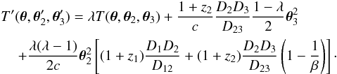17)

The second term in Eq. (17) only depends on the source position θ₃; therefore, this term does not contribute to the time delay, which is obtained as the difference of T between images. The third term of Eq. (17) vanishes, since the expression in the bracket is zero because of relations between the D’s – see Schneider et al. (1992). We thus find that all time delays in a two-source plane lens scale with λ under an MST, for sources on both source planes. Hence, time-delay ratios do not break the degeneracy of the MST; on the other hand, any time delay from a source in either source plane breaks it, provided H₀ is assumed to be known.

3. Cosmology from two-source plane lensing?

In the light of the new MST, we now consider the possibility of constraining cosmological parameters from two-source plane lenses. In the approach of CA14, the sensitivity to cosmology is due to the distance ratio parameter β, which depends on the density parameters and the dark energy e.o.s. parameter w. Different cosmological models yield different distance-redshift relations, and thus different β. Thus let β correspond to a fiducial cosmological model, and β′ to a model with different parameters. We examine below whether we can find deflection angles ${{\alpha }}_{\mathit{i}}^{\mathrm{\prime }}\mathrm{\left(}{{\theta }}_{\mathit{i}}^{\mathrm{\prime }}\mathrm{\right)}$ such that the lens mappings are unchanged between the fiducial and modified models, up to a uniform scaling (by a factor ν_i) in the lens/source planes. Thus we require for the first lens equation ${{\theta }}_{\mathrm{2}}^{\mathrm{\prime }}\mathrm{=}{\theta }\mathrm{-}{\mathit{\beta }}^{\mathrm{\prime }}{{\alpha }}_{\mathrm{1}}^{\mathrm{\prime }}\mathrm{\left(}{\theta }\mathrm{\right)}\mathrm{=}{\mathit{\nu }}_{\mathrm{2}}{{\theta }}_{\mathrm{2}}\mathrm{=}{\mathit{\nu }}_{\mathrm{2}}\left[{\theta }\mathrm{-}\mathit{\beta }{{\alpha }}_{\mathrm{1}}\mathrm{\left(}{\theta }\mathrm{\right)}\right]\mathit{.}$(18)With the ansatz 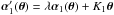${{\alpha }}_{\mathrm{1}}^{\mathrm{\prime }}\mathrm{\left(}{\theta }\mathrm{\right)}\mathrm{=}\mathit{\lambda }{{\alpha }}_{\mathrm{1}}\mathrm{\left(}{\theta }\mathrm{\right)}\mathrm{+}{\mathit{K}}_{\mathrm{1}}{\theta }$, we obtain by comparing terms in Eq. (18) proportional to α₁ and θ the two relations β′λ = ν₂β and 1 − β′K₁ = ν₂, with solutions ν₂ = β′λ/β and K₁ = 1 /β′ − λ/β. The requirement for the second lens equation reads ${{\theta }}_{\mathrm{3}}^{\mathrm{\prime }}\mathrm{=}{\theta }\mathrm{-}{{\alpha }}_{\mathrm{1}}^{\mathrm{\prime }}\mathrm{\left(}{\theta }\mathrm{\right)}\mathrm{-}{{\alpha }}_{\mathrm{2}}^{\mathrm{\prime }}\mathrm{\left(}{{\theta }}_{\mathrm{2}}^{\mathrm{\prime }}\mathrm{\right)}\mathrm{=}{\mathit{\nu }}_{\mathrm{3}}{{\theta }}_{\mathrm{3}}\mathrm{=}{\mathit{\nu }}_{\mathrm{3}}\left[{\theta }\mathrm{-}{{\alpha }}_{\mathrm{1}}\mathrm{\left(}{\theta }\mathrm{\right)}\mathrm{-}{{\alpha }}_{\mathrm{2}}\mathrm{\left(}{{\theta }}_{\mathrm{2}}\mathrm{\right)}\right]\mathit{.}$(19)Inserting the ansatz

${{\alpha }}_{\mathrm{2}}^{\mathrm{\prime }}\mathrm{\left(}{{\theta }}_{\mathrm{2}}^{\mathrm{\prime }}\mathrm{\right)}\mathrm{=}{\mathit{\nu }}_{\mathrm{3}}{{\alpha }}_{\mathrm{2}}\mathrm{(}{{\theta }}_{\mathrm{2}}^{\mathrm{\prime }}\mathit{/}{\mathit{\nu }}_{\mathrm{2}}\mathrm{)}\mathrm{+}{\mathit{K}}_{\mathrm{2}}{{\theta }}_{\mathrm{2}}^{\mathrm{\prime }}\mathrm{=}{\mathit{\nu }}_{\mathrm{3}}{{\alpha }}_{\mathrm{2}}\mathrm{(}{{\theta }}_{\mathrm{2}}^{\mathrm{\prime }}\mathit{/}{\mathit{\nu }}_{\mathrm{2}}\mathrm{)}\mathrm{+}{\mathit{K}}_{\mathrm{2}}{\mathit{\nu }}_{\mathrm{2}}\left[{\theta }\mathrm{-}\mathit{\beta }{{\alpha }}_{\mathrm{1}}\mathrm{\left(}{\theta }\mathrm{\right)}\right]$into Eq. (19), the comparison of terms propotional to α₁ and θ yields the equations λ − K₂ν₂β = ν₃ and 1 − K₁ − K₂ν₂ = ν₃, which have the solutions 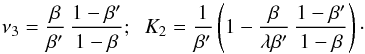${\mathit{\nu }}_{\mathrm{3}}\mathrm{=}\frac{\mathit{\beta }}{{\mathit{\beta }}^{\mathrm{\prime }}}\hspace{0.17em}\frac{\mathrm{1}\mathrm{-}{\mathit{\beta }}^{\mathrm{\prime }}}{\mathrm{1}\mathrm{-}\mathit{\beta }}\mathrm{;}{\mathit{K}}_{\mathrm{2}}\mathrm{=}\frac{\mathrm{1}}{{\mathit{\beta }}^{\mathrm{\prime }}}\left(\mathrm{1}\mathrm{-}\frac{\mathit{\beta }}{\mathit{\lambda }{\mathit{\beta }}^{\mathrm{\prime }}}\hspace{0.17em}\frac{\mathrm{1}\mathrm{-}{\mathit{\beta }}^{\mathrm{\prime }}}{\mathrm{1}\mathrm{-}\mathit{\beta }}\right)\mathrm{·}$(20)Hence we see that a change of cosmology changes the lens equations in a similar way as an MST. Even with a change in β, we retain the freedom of a one-parameter family of mass models that leave the lens mapping invariant, up to a uniform scaling. In contrast to the MST discussed in Sect.2.3, here a non-trivial scaling of the second lens plane is implied, where ν₃ solely depends on change of β.

Three special choices of λ are worth to be discussed separately: (1) No mass sheet in the first lens plane (NMS1): for λ = β/β′, K₁ = 0 and ν₂ = 1, so that there is no mass sheet in the first lens and no scaling in the first source/second lens plane is implied. The mass sheet in the second lens plane then becomes K₂ = (β′ − β)/ [β′(1 − β)]. For four different variations around a fiducial cosmological model, all with zero spatial curvature, we give the values of β′, K₂ and ν₃ in Table1, using the redshifts for the system SDSSJ0946+1006 (setting the uncertain redshift of the second source to be z₃ = 2.4). (2) No mass sheet in the second lens plane (NMS2): setting λ = ν₃, we derive K₂ = 0, ν₂ = (1 − β′)/(1 − β), and K₁ = (β′ − β)/ [β′(1 − β)], so that λ + K₁ = 1. Hence, in this case, there is no mass sheet in the second lens plane, and the one in the first lens plane is the same as K₂ was for NMS1. (3) Equal-mass scaling (EMS): choosing sheets of equal density in both lens planes, we derive $\mathit{\lambda }\mathrm{=}\mathrm{(}\mathit{\beta }\mathit{/}{\mathit{\beta }}^{\mathrm{\prime }}\mathrm{)}\sqrt{\mathrm{(}\mathrm{1}\mathrm{-}{\mathit{\beta }}^{\mathrm{\prime }}\mathrm{)}\mathit{/}\mathrm{(}\mathrm{1}\mathrm{-}\mathit{\beta }\mathrm{)}}$, ${\mathit{K}}_{\mathrm{1}}\mathrm{=}{\mathit{K}}_{\mathrm{2}}\mathrm{=}\mathrm{(}\mathrm{1}\mathrm{-}\sqrt{\mathrm{(}\mathrm{1}\mathrm{-}{\mathit{\beta }}^{\mathrm{\prime }}\mathrm{)}\mathit{/}\mathrm{(}\mathrm{1}\mathrm{-}\mathit{\beta }\mathrm{)}}\mathrm{)}\mathit{/}{\mathit{\beta }}^{\mathrm{\prime }}$, and ${\mathit{\nu }}_{\mathrm{2}}\mathrm{=}\sqrt{\mathrm{(}\mathrm{1}\mathrm{-}{\mathit{\beta }}^{\mathrm{\prime }}\mathrm{)}\mathit{/}\mathrm{(}\mathrm{1}\mathrm{-}\mathit{\beta }\mathrm{)}}$. For these choices of λ, we also list some quantities for the different cosmological parameters in Table1.

From the table, we see that variations of the cosmological parameters within generous plausible ranges yield only small deviations of β′ from β. Correspondingly, the required MSTs are small; for the three special choices discussed above they imply mass sheets with | K_i | < 0.06. In particular, for EMS, the mass-sheet densities are smaller than 0.03. Such low values of K_i are perfectly acceptable, even if fairly accurate measurements of the velocity dispersion of the lenses were available (see Schneider & Sluse 2013, for a more detailed discussion). In particular, if the original mass distribution were a power law, the transformed ones ${\mathit{\kappa }}_{\mathit{i}}^{\mathrm{\prime }}$ would deviate only very little from a power law over the range where multiple images are formed.

4. Discussion

We have shown that a lens system with two lens and two source planes admits a mass-sheet transformation that leaves the lens mapping invariant up to a uniform scaling in the source and lens plane(s). Furthermore, we demonstrated in the previous section that a change of cosmological parameters is essentially equivalent to an MST. A mass sheet acts like a magnifying glass, changing apparent distances, much in the same way as a different expansion history changes the distance-redshift relation. For the particular case of SDSSJ0946+1006 (Gavazzi et al. 2008), we have shown that the changes of the mass distribution in the second lens plane are very small when the cosmological parameters are changed within currently acceptable ranges.

As explicitly stated in CA14, the cosmological constraints they obtained are based on the assumption of a power-law mass distribution in either lens planes. This assumption about the functional form of the density profile formally breaks the degeneracy implied by the MST, but there are no good reasons to assume that the profiles of galaxies are exactly described by a power law (see Schneider & Sluse 2013). Indeed, the case NMS1 discussed above implies no added mass sheet in the first lens plane, thus preserving the power-law property, whereas the case EMS corresponds to only small K_i, yielding only marginal modifications of the power-law mass profile. The MST also for multiple source and lens planes provides a degeneracy in the determination of lens-mass distributions and cosmological distance ratios in lens systems, and needs to be accounted for in future studies.

Acknowledgments

The author thanks Dominique Sluse, Tom Collett, Sherry Suyu, and an anonymous referee for helpful discussions and comments on the manuscript. This work was supported in part by the Deutsche Forschungsgemeinschaft under the TR33 “The Dark Universe”.

References

All Tables

References

- Bartelmann, M. 2010, Class. Quant. Gravity, 27, 3001 [Google Scholar]
- Bradač, M., Lombardi, M., & Schneider, P. 2004, A&A, 424, 13 [NASA ADS] [CrossRef] [EDP Sciences] [Google Scholar]
- Coe, D., Fuselier, E., Benítez, N., et al. 2008, ApJ, 681, 814 [NASA ADS] [CrossRef] [Google Scholar]
- Collett, T. E., & Auger, M. W. 2014, MNRAS, 443, 969 [NASA ADS] [CrossRef] [Google Scholar]
- Collett, T. E., Marshall, P. J., Auger, M. W., et al. 2013, MNRAS, 432, 679 [NASA ADS] [CrossRef] [Google Scholar]
- Falco, E. E., Gorenstein, M. V., & Shapiro, I. I. 1985, ApJ, 289, L1 [Google Scholar]
- Gavazzi, R., Treu, T., Koopmans, L. V. E., et al. 2008, ApJ, 677, 1046 [NASA ADS] [CrossRef] [Google Scholar]
- Greene, Z. S., Suyu, S. H., Treu, T., et al. 2013, ApJ, 768, 39 [NASA ADS] [CrossRef] [Google Scholar]
- Kochanek, C. S. 2006, in Saas-Fee Advanced Course 33: Gravitational Lensing: Strong, Weak and Micro, eds. G. Meylan, P. Jetzer, P. North, et al., 91 [Google Scholar]
- Liesenborgs, J., & De Rijcke, S. 2012, MNRAS, 425, 1772 [NASA ADS] [CrossRef] [Google Scholar]
- Liesenborgs, J., de Rijcke, S., Dejonghe, H., & Bekaert, P. 2008, MNRAS, 386, 307 [NASA ADS] [CrossRef] [Google Scholar]
- Refsdal, S. 1964, MNRAS, 128, 307 [NASA ADS] [CrossRef] [Google Scholar]
- Schneider, P., & Sluse, D. 2013, A&A, 559, A37 [NASA ADS] [CrossRef] [EDP Sciences] [Google Scholar]
- Schneider, P., Ehlers, J., & Falco, E. E. 1992, Gravitational Lenses (New York, Heidelberg: Springer Verlag) [Google Scholar]
- Suyu, S. H., Auger, M. W., Hilbert, S., et al. 2013, ApJ, 766, 70 [NASA ADS] [CrossRef] [Google Scholar]
- Treu, T. 2010, ARA&A, 48, 87 [NASA ADS] [CrossRef] [Google Scholar]
- Wong, K. C., Keeton, C. R., Williams, K. A., Momcheva, I. G., & Zabludoff, A. I. 2011, ApJ, 726, 84 [NASA ADS] [CrossRef] [Google Scholar]
All Tables
Current usage metrics show cumulative count of Article Views (full-text article views including HTML views, PDF and ePub downloads, according to the available data) and Abstracts Views on Vision4Press platform.
Data correspond to usage on the plateform after 2015. The current usage metrics is available 48-96 hours after online publication and is updated daily on week days.
Initial download of the metrics may take a while.