| Issue |
A&A
Volume 568, August 2014
|
|
|---|---|---|
| Article Number | A89 | |
| Number of page(s) | 11 | |
| Section | Extragalactic astronomy | |
| DOI | https://doi.org/10.1051/0004-6361/201424279 | |
| Published online | 26 August 2014 | |
Probing the nuclear star cluster of galaxies with extremely large telescopes
1 INAF, Osservatorio Astronomico di Padova, Vicolo dell’Osservatorio 5, 35122 Padova, Italy
e-mail: This email address is being protected from spambots. You need JavaScript enabled to view it.
2 INAF, Osservatorio Astronomico di Bologna, Via Ranzani 1, 40127 Bologna, Italy
3 INAF, Istituto di Astrofisica Spaziale e Fisica Cosmica, Via Bassini 15, 20133 Milano, Italy
Received: 26 May 2014
Accepted: 23 June 2014
Abstract
The unprecedented sensitivity and spatial resolution of next-generation, ground-based, extremely large telescopes (ELTs) will open a completely new window on the study of resolved stellar populations. In this paper we study the feasibility of the analysis of nuclear star cluster (NSC) stellar populations with ELTs. To date, NSC stellar population studies are based on the properties of their integrated light. NSCs are in fact observed as unresolved sources even with the HST. We explore the possibility of obtaining direct estimates of the age of NSC stellar populations from the photometry of main-sequence turn-off stars. We simulated ELT observations of NSCs at different distances and with different stellar populations. Photometric measurements on each simulated image were analysed in detail and results about photometric accuracy and completeness are reported here. We found that the main-sequence turn-off is detectable – and therefore the age of stellar populations can be directly estimated – up to 2 Mpc for old, up to 3 Mpc for intermediate-age and up to 4−5 Mpc for young stellar populations. We found that for this particular science case, the performances of TMT and E-ELT are of comparable quality.
Key words: instrumentation: adaptive optics / instrumentation: high angular resolution / galaxies: clusters: general / infrared: stars / methods: observational
© ESO, 2014
1. Introduction
The nuclei of galaxies are extraordinary laboratories to probe the processes that lead to the formation of nowadays galaxies. The properties of the nuclear regions are in fact thought to be linked with the formation history of the galaxies where the collapse of gas and merging events may play a relevant role for different types of galaxies and environments. Various phenomena characterise these nuclei such as super-massive black holes (SMBHs), active galactic nuclei, central starbursts, and extreme stellar densities. All these phenomena are likely connected to the global properties of their host galaxies, and co-evolution of the various components is invoked to account for the observed correlations.
For instance, important links between the mass of the central SMBH and the global properties of the host galaxies have been discovered (see e.g. Ferrarese et al. 2006; Wehner & Harris 2006; Neumayer & Walcher 2012; Scott & Graham 2013, and refs therein). Another less explored phenomenon is the presence of compact and massive star clusters found in the centres of most of nearby galaxies of all morphological types (see e.g. Böker 2010). The formation of nuclear star clusters (NSC) may also be connected to the formation of SMBH in the centre, and these objects could therefore trace the evolution history of the whole galaxy formation. For example, NSCs sit on the low mass extrapolation of the scaling relation between the SMBH mass and the total mass of the host galaxy.
Photometry of NSCs in a large sample of spiral galaxies has been investigated by Böker et al. (2002) and, more recently, by Georgiev & Böker (2014). NSCs in spheroidal galaxies has been studied by Côté et al. (2006) and Turner et al. (2012). NSCs are 3−4 mag (Georgiev & Böker 2014) more luminous than Milky Way globular clusters, but they share similar sizes (a few parsecs, see e.g. Böker et al. 2004). Their estimated total mass (106 − 107 M⊙; Böker 2010) is at the high end of the globular clusters’ mass function.
Two main scenarios have been suggested for the formation of NSCs: i) infall of star clusters that formed elsewhere in the host galaxy (Tremaine et al. 1975; Capuzzo-Dolcetta & Miocchi 2008); ii) in situ formation and build-up through star formation following the accretion of gas in the centre of the galaxies. Bekki (2007) performed chemodynamical simulations of the inner regions of dwarf galaxies, where dissipative merging of stellar and gaseous clumps formed in the spiral arms can lead to the formation of NSCs. According to this model the metallicity of the stars in the NSC would be higher than that of its host spheroid. In addition, in these models the time scale of cluster formation is shorter for higher masses, and therefore one expects that less massive galaxies should host younger NSCs.
A detailed study of the stellar populations in NSCs therefore appears a key tool for understanding the main physical processes involved in the formation and growth of these stellar systems. However, current instrumentation allows us to investigate this issue only from observations of the NSCs integrated light. Ages, metallicities, and in general, star formation histories are inferred from integrated colours, indices, and/or spectral energy distribution fitting techniques (see e.g., Walcher et al. 2006; Seth et al. 2006, 2010; Rossa et al. 2006). In fact even with the HST capabilities, it is not possible to resolve the stars of NSCs beyond the Local Group (see e.g. Böker et al. 2002)1. The derived properties of the stellar population are thus based on population synthesis models, and results are therefore affected by uncertainties intrinsically related to the models, like the age-metallicity degeneracy, as well as the difficulty of separating different age components. In particular the presence of young stars strongly limits the accuracy of the age and metallicity estimate of unresolved stellar systems because the young component dominates the integrated light, even when representing a small contribution to the mass of the whole stellar system.
Recent studies from HST spectroscopic observations (Paudel et al. 2011) of early-type dwarf galaxies in the Virgo cluster suggest that many nuclei contain a stellar population that is significantly younger (by ~3 Gyr) and more metal-rich than that of the host galaxy. This would indicate that NSCs formed after the main body of the host galaxy, likely from mergers of gas clumps. However in a small number of cases the nuclei are found to be dominated by older and more metal poor stellar population than that of their host galaxies, thus favouring the merging scenario of old pre-existing star clusters. These differences could be reconciled if different mechanisms were invoked for NSCs in galaxies of different mass. For example, from the study of the surface brightness profiles of a sample of ~40 early-type galaxies in the Fornax cluster, Turner et al. (2012) suggest that the formation of NSCs occurs via merging of pre-existing clusters in lower mass galaxies, via gas accretion in higher mass hosts.
The emerging picture from these studies is limited by the use of the integrated light of the stellar systems and significant advancement in recovering the star formation history of the nuclei of these galaxies can be derived from the photometry of individual stars. The analysis of the colour–magnitude diagram (CMD) of the resolved stars is in fact the most direct way to estimate the age and the metallicity of stellar populations. Indeed, isochrone fitting of the turn off region is the optimal tool to derive the age, while the colour of the red giant branch stars is a good estimator of the metallicity (see e.g. Greggio & Renzini 2011). In addition, resolving individual stars would yield a direct information on the multiplicity of star formation events, or on the duration of the episodes of star formation in the NSCs.
Given the high surface density of stars in NSCs and the large distance of their host galaxies, the construction of CMDs of stars is well beyond the capabilities of present-day instrumentation but will become feasible with the next generation of extremely large telescopes (ELTs) – as the European-ELT (E-ELT)2, the Thirty Meter Telescope (TMT)3, the Grand Magellan Telescope (GMT)4 – that will join high sensitivity with extraordinary (a few mas) spatial resolution, when coupled with adaptive optics. In particular, the unprecedented spatial resolution of adaptive-optics ELTs (3−5 mas) will open a new window in the study of crowded stellar fields. It will be possible, for the first time, to obtain resolved stellar photometry in NSCs beyond the Local Group yielding direct measurements of stellar ages and metallicities. We will then be in the condition to provide strong constraints to the physical models of NSC formation and to understand what are the connections between the formation and evolution of central massive objects and their host galaxy.
In this paper we explore in detail the capabilities of studying the stellar population of NSCs in nearby galaxies (up to 4 Mpc) using simulated near-infrared (IR) imaging observations of future ELTs. In particular we adopt as baseline the parameters of Multi-AO Imaging Camera for Deep Observations (MICADO; Davies et al. 2010) proposed for E-ELT and compare the results to those obtainable with the InfraRed Imaging Spectrograph (IRIS; Larkin et al. 2010) foreseen for the TMT. The results are also compared with the expected capabilities of the Near Infrared Camera (NIRCam; Greene et al. 2010) to be mounted at the James Webb Space telescope (JWST) that may reach similar sensitivity but with worse angular resolution.
The paper is organised as follows: Sect. 2 describes our simulated observations of NSCs. Section 3 describes the procedure we adopted to extract photometric catalogues from the simulated images and the analysis of the photometric accuracy. Section 4 presents an analysis of the feasibility of the science case with other next-generation instrumentation. A summary of this work and our conclusions are presented in Sect. 5.
2. Simulation of NSCs in galaxies
In order to age-date the resolved stellar population of the NSC we need to disentangle the cluster members from the stars of its host galaxy. In the central parts of the cluster, the stellar field is dominated by the cluster members, but the stellar density is very high and stars are blended, decreasing the accuracy of the photometry. On the other hand, in the external regions, where photometry is more accurate, the host galaxy body population contribution becomes important, and it is more difficult to disentangle the two components. The interplay of these two factors determines the intermediate region where photometry can be accurate enough and the host contribution is low enough to allow us to measure reliable age and metallicity for the cluster stellar populations. Thus, the possibility of characterising the stellar population of NSCs depends on a few parameters, e.g. the distance of the host galaxy and the core radius of the cluster which control the crowding conditions. In addition, for a given distance, the older the NSC the fainter are the stars at the turn off, which makes it more difficult to determine its age. In order to exploit the capabilities of ELTs to investigate NSCs, we have considered a number of cases with different age and at different distance.
2.1. The input stellar populations
As baseline for the simulations we adopted NGC 300 as a NSC-host template galaxy. This late-type galaxy located at 2 Mpc is one of the closest galaxies known to host a NSC. Böker et al. (2004) found that the NSC in NGC 300 follows a King profile with a tidal radius  and core radius
  . The resulting half-light radius is
  . Using a single age and single metallicity stellar population (simple stellar population, SSP) model, the age of the stellar population in the NSC is estimated to be ~1 Gyr. Allowing for an extended star formation period, the data support a luminosity-weighted mean age of 3 Gyr and a wide range in age. The NSC metallicity is estimated of Z = 0.004 and the total mass of M = 106 M⊙ (Rossa et al. 2006; Walcher et al. 2006).
In the simulated frames, the input stellar population consists of a combination of two components, one for the host galaxy body, described as a composite stellar population, and one for the NSC, described as a SSP. While there is no guarantee that the NSCs are really SSPs, our simulations will show how well the simplest case of NSC stellar population can be characterised in terms of age and metallicity. More complicated star formation histories can be viewed as the superposition of several individual episodes of star formation.
For the host galaxy body stellar population we adopted the model used in Greggio et al. (2012) as representative of a typical disk of a late-type galaxy. The model has a constant star formation rate over the last 12 Gyr and a chemical evolution with the metallicity linearly increasing from Z = 0 up to the solar value in the first 5 Gyrs. Later on, the chemical enrichment is assumed much slower, with the metallicity reaching Z = 0.02 for the youngest stars. The surface density of stars for the host-galaxy body component was chosen so as to reproduce a central surface brightness of μB = 20.4 mag arcsec-2. For the adopted galaxy model, this corresponds to surface brightness of 18.88, 17.98, 17.27, and 17.13 mag arcsec-2 in the I, J, H, and K bands, respectively. These values are close to those measured for NGC 300 (see e.g. Böker et al. 2002).
Parameters of the SSPs used to simulate the NSCs: age, metallicity, total number of stars, I-band absolute magnitude, and total mass at birth.
We chose an SSP model to describe the stellar population of the NSC, for which we considered three age values, 1, 4, and 10 Gyr. This allowed us to probe the dependence of the results on the NSC age. The synthetic SSP was created by distributing objects along stellar isochrones from Marigo et al. (2008) provided by the CMD v2.5 web tool5. We adopted a Salpeter initial mass function from 0.5 M⊙ to the mass of the star at the tip of the asymptotic giant branch (AGB). The contribution to the total luminosity of stars with masses below 0.5 M⊙ is negligible (≲5% for all considered cases in all considered bands, assuming a flat initial mass function below 0.5 M⊙). The main properties of the input SSPs used to simulate the NSCs are summarised in Table 1.
The dependence of the results on the galaxy distance was tested by putting our synthetic populations at 2 and 4 Mpcs. The simulated NSC stars have been distributed following a King-profile model; for the simulations of the systems at 2 Mpc we assumed the structural parameters of the NSC in NGC 300 (see above), while for those at 4 Mpc we adopted  and
and  , consistently scaled from those of the NSC in NGC 300.
2.2. Simulated images
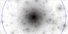 |
Fig. 1 Zoom of a 6″ × 3″ region of the J-band simulated MICADO@E-ELT image of the 1 Gyr old NSC located at 2 Mpc. The circles show the effective radius ( |


We simulated observations with two instruments, MICADO@E-ELT and IRIS@TMT following the specifications in Davies et al. (2010) and Wright et al. (2010).
MICADO (Multi-AO Imaging Camera for Deep Observations) is a phase A imaging instrument designed for E-ELT to provide diffraction limited imaging over a wide (~1 arcmin) field of view. The simulations of MICADO observations in I, J, H, and K-bands were performed assuming a primary mirror with a diameter of 39 meters and a 28% obscuration. We assumed a total throughput of 39% in the I and K bands and 40% in J and H bands. We used a read noise of 5 e− and a pixel scale 3 mas. We assumed the typical near-IR sky background measured at Cerro Paranal and included the contribution of thermal emission in the near-IR-bands; specifically we adopted a total background of 20.0, 16.3, 15.0, and 12.8 mags/arcsec-2 in the I, J, H, and K bands, respectively. Under these conditions the signal-to-noise of isolated point sources of magnitude 26−28 is dominated by the contribution of the background while read-out noise is negligible. This allows one to obtain several individual frames of the same field in order to avoid saturation and properly subtract the bright IR background. We used the last version (June 2012) of the point spread functions (PSFs) of the multi conjugate adaptive optics post focal relay (MAORY; Diolaiti et al. 2010) calculated for a  seeing at the centre of the corrected field of view (FoV), as provided by the MAORY official website6.
The InfraRed Imaging Spectrograph (IRIS; Larkin et al. 2010) is one of the first-light instruments designed for the TMT. TMT is a 30 m telescope that will be mounted at Mauna Kea, Hawaii, USA. It will observe in the wavelength range from 0.31 to 20 μm. IRIS will have both imaging and integral field spectroscopy capabilities with a spectral coverage from 0.84 μm to 2.4μm. The imager has 4 mas pixels and a field of view of  and will be equipped with Z, Y, J, H, and K filters. A full description of the IRIS instrument and its performances can be found in Wright et al. (2010) and Do et al. (2014). We simulated IRIS observations using the input star list (magnitudes and positions on the frame) generated for the MICADO images for the 1 Gyr old SSP at 2 Mpc distance (details in Sect. 4). Images were produced using the PSFs kindly provided by S. Wright and the NFIRAOS Team (see Do et al. 2014). TMT observations have been simulated in the Z and J band only.
All simulated images were produced using the AETC7 v.3.0 tool (Falomo et al. 2011) using a total integration time of 3h. We simulated a simple observing strategy, with no dithering because the PSF core is well sampled in J, H, and K bands and slightly undersampled in the I band (the FWHM of the PSF core is 1.8 pixels). The impact of this on the I-band photometric accuracy is not a major issue (see Sect. 3.1). The size of the images was set much larger than the tidal radius of the NSC. For simulations at 2 Mpc we produced images with a  FoV; at 4 Mpc we reduced the size to
  . An example of a simulated image is shown in Fig. 1.
3. Photometry on E-ELT images
The photometric analysis of the simulated images was performed using Starfinder (Diolaiti et al. 2000), a photometric package specifically designed for high resolution AO images. One of the key-features of Starfinder is that it creates a 2D image of the PSF using bright and isolated stars, without any analytic approximation. This is particularly important since the PSF in AO systems is highly structured; therefore it cannot be accurately described as a combination of a few analytical components (see for details Schreiber et al. 2012). Starfinder was already tested and proved to provide excellent results on E-ELT simulated images (Deep et al. 2011; Schreiber et al. 2014).
The photometric analysis was performed assuming we had no a priori knowledge of the PSF, simulating the photometric reduction of real observations. We set a detection limit of 3σ above the local background as the threshold for object detection. Firstly, we masked out the crowded central region of the NSC in the image. Then, a rough estimate of the background level was obtained as the median value of the image and the PSF was estimated from 50 bright and relatively isolated stars. The background level and the PSF estimates were then refined using an iterative procedure. Each step consists of the following four operations:
-
evaluation of the average value of the background and itssubtraction from the image;
-
estimation of a new PSF from 50 bright and isolated stars after subtracting all neighbouring stars ;
-
fitting of all sources detected at 3σ level above the local background with the PSF model;
-
calculation of a residual image obtained by subtracting all fitted stars from the original image; this image was then used to obtain an improved estimate of the background.
This procedure was iterated until the background value and the PSF model converge to the final values, i.e. the variations with respect to the previous iteration were less than 1% (in all cases this happened after four iteration). The final source detection and fitting was performed on the original image, including the central region previously masked out.
The photometric catalogues were cross-correlated with the input catalogues with a matching radius of 1 pixel. As a first step in our matching procedure we sorted the photometric catalogue by increasing magnitudes (from bright to faint objects). When more than one input star was found within 1 pixel from a measured source, the brightest input star was chosen. The matched input star was removed from the catalogue and the procedure proceeded with the next star. The zero-point of the photometry was derived as the median difference between the input and the measured magnitudes of the 300 brightest stars located beyond the tidal radius of the NSC. This was done because in the crowded central regions the stars are systematically affected by a zero-point offset due to blending of two or more sources. This issue will be addressed in the next sections.
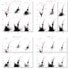 |
Fig. 2 Colour–magnitude diagrams of different regions of the simulated stellar system obtained from MICADO simulations. The lines are the isochrones from Marigo et al. (2008) representative of the nuclear cluster stars. The red line is the MS and the RGB, while the blue line is the sequence of core He-burning stars, up to the first thermal pulse on the AGB. The upper-left sub-panels show the CMDs of the input stellar catalogues (NSC plus host galaxy main body). For clarity only stars in the inner 3re region are shown. |
Some examples of CMDs obtained from the simulated images are shown in Fig. 2 where the solid lines in each panel show the locus described by the input stellar population. The CMDs of the input stellar catalogues are also shown for reference. In the crowded central regions of the clusters stellar blends strongly decrease the photometric accuracy. Photometric errors are extremely large and the photometry is much shallower than in the outer regions. As a consequence the CMDs in the central region cannot be used to study the NSC stellar populations. Going towards larger radii, the CMD becomes progressively more populated with the underlying galaxy component, until the CMDs in the external regions are mainly populated by host galaxy members, as the surface density of NSC stars is very low. The CMDs of the regions at 5re<r<rt are in fact undistinguishable from those of the regions beyond the NSC tidal radius, populated only by members of the host galaxy. The NSC stellar populations are clearly visible in the intermediate regions, between 3 and 5re. This is especially true for the cases with a 1 Gyr old NSC, at both 2 and 4 Mpc distance. The brightest part of the red-giant branch (RGB) and the red clump (RC) are visible in all CMDs. The main-sequence turn-off (MSTO) is clearly visible in the most favourable cases (e.g. 1 Gyr old SSP at 2 Mpc distance), but completely undetectable for the oldest SSP at 4 Mpc. In the intermediate cases, detection of the NSC MSTO is complicated by the presence of the host galaxy population. The main goal of this paper is to study under which conditions it is possible to observe NSC MSTO stars. To this end, it is necessary to assess whether the contamination by foreground host galaxy stellar populations prevents the detection or not. We discuss this in Sect. 3.3.
3.1. Photometric errors
The photometric accuracy was analysed by computing the difference between the measured magnitudes and the input ones. The differences between the observed and the input magnitude, that will be referred to as photometric errors, are strongly dependent on the crowding conditions and on the magnitude of the star. When crowding is negligible, photometric errors are dominated by the statistic of the counts and their distribution is expected to be symmetric, with null median value and a dispersion increasing with the input magnitudes. As the stellar crowding grows, the probability of blending of two or more sources increases; consequently the magnitudes of the stars are more frequently recovered brighter than input ones and the resulting photometric error distribution is skewed towards negative values (see e.g. Greggio & Renzini 2011). In this section we study the photometric error distribution as a function of the radial distance from the NSC centre; in particular we will determine at which distance from the cluster centre crowding conditions prevent reliable photometric measurements.
For each simulation, we divided the stars in three groups, according to the radial distance from the cluster centre. We computed the median of the photometric errors and the 1σ widths of the error distributions binning data in 0.2 mag intervals (excluding bins with less than 50 stars). The dispersions of the errors in each magnitude bin were computed independently for the stars measured brighter (σ−) and those measured fainter (σ+) than the input magnitudes. On the basis of the arguments presented above, the median and the σ− values trace the effect of blending, while σ+ is an indicator of the contribution to the photometric uncertainties of random factors, i.e. mainly photon and read-out noise.
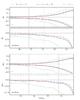 |
Fig. 3 Photometric errors in the simulation at 2 Mpc with the 1 Gyr old clusters in I and H-band. The first and third panels from the top show the σ+ (upper curves) and σ− (lower curves) values for each radial distance bin. The other two panels show the median error. The two vertical lines show the magnitude of the RC and the MSTO. |
Figure 3 shows the photometric errors obtained for the simulated images with the 1 Gyr old cluster at 2 Mpc. This case is used as an example, and the following considerations and the general results also apply to the other simulations. We note that the error distribution in the outer region of the cluster (5 <r/re< 10) is almost identical to that in the very external regions, beyond the cluster tidal radius (r>rt), over the whole magnitude range probed. This means that the photometric accuracy in the outer part of the cluster is the same as in the region beyond the tidal radius, where no cluster members are present. In other words, the crowding affects the photometric errors only at radial distances r ≲ 5re. It is interesting to note that photometric errors for the brightest sources are smaller in the reddest bands; the σ+ and σ− are in fact ~0.03 mag in the I band, and ≲0.01 mag in H. This is because the AO correction is more efficient at longer wavelengths, leading to a higher Strehl ratio in redder bands (Ciliegi et al. 2012). Moreover the I-band images are slightly under-sampled (the FWHM of the PSF core in the I-band is ~1.8 pixels). On the other hand, the photometric errors for faintest stars –at the level of the MSTO– are smaller in the blue bands. This is due to the lower background noise in the I-band images.
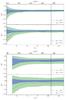 |
Fig. 4 Photometric errors for the simulation at 2 Mpc (upper panels) and 4 Mpc (lower panels) in the I and J bands for stars at magnitudes corresponding to the 1 Gyr MS turn-off and red-clump. The vertical line corresponds to the NSC tidal radius. |
Figure 4 shows the dependence on distance from the cluster centre of the width of the error distribution at the MSTO magnitude and at the clump magnitude for the case of a 1 Gyr old SSP at 2 and 4 Mpc distance. As seen before the dispersion of the photometric errors distribution decreases at increasing radial distances in the central region of the cluster. In the outer region the stellar surface density is lower and therefore the effects of stellar blending on the photometric accuracy are negligible. As a consequence, beyond a critical radial distance the photometric errors (both σ− and σ+) are constant. For MSTO stars this critical radial distance is ~5re at 2 Mpc and ~6re at 4 Mpc for the 1 Gyr old case. For the 4 Gyr NSC the critical radius for MSTO stars is larger, because the MSTO is fainter. Specifically the radius is ~6re and ~7re respectively for the simulations at 2 and 4 Mpc. For the 10 Gyr old NSC the MSTO at 4 Mpc is not detected, while at 2 Mpc it is at the detection limit.
3.2. Completeness
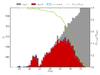 |
Fig. 5 I-band luminosity function of all input stars (grey) and of input stars position-matched with a source in the output catalogue (red). We also plotted the LF obtained from the measured magnitudes in the output catalogue (blue). The completeness function is shown by the green line and its scale is shown on the right-hand axis. The LFs are computed from stars with a radial distance between 3.5re and 4.5re in the images of the 1 Gyr old cluster at 2 Mpc. |
Figure 5 shows stellar luminosity functions (LF) for the simulation of the 1 Gyr old cluster at 2 Mpc. Specifically, the input luminosity function is shown as a grey histogram; the red histogram is the LF of all input stars that were found, i.e. position-matched with a source detected by Starfinder. This LF is plotted as function of the input magnitudes. The open blue histogram is the output LF, function of the measured magnitude. The difference between the last two LFs is due to photometric errors. We define as completeness factor the ratio between the first two LFs, Nfound/Ninput. We note that no selection on the photometric error was applied to build the LFs used to define the completeness. The completeness is therefore the probability that a star with a given input magnitude is recovered by our reduction procedure, i.e. matched with a measured star, irrespective of its photometric error. The completeness curve is shown as a green line in Fig. 5 and its scale is drawn on the right-hand axis.
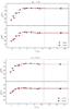 |
Fig. 6 The 50% completeness magnitude as a function of the radial distance from the NSC centre. The vertical line is the NSC tidal radius. Results for the simulations with the 1 and 10 Gyr old clusters are shown in the upper and lower panels respectively. |
We characterise the photometric depth as the magnitude level at which a 50% completeness factor is reached (mag50%). Figure 6 shows mag50% as a function of the radial distance from the NSC centre for the simulations with the young star cluster. At small radial distances from the cluster centre the photometry is clearly shallower than in the external regions because of the extreme crowding conditions. At increasing radial distances the stellar density decreases and the photometry is progressively deeper. Beyond a certain radius the stellar crowding is not the dominant factor that determine the photometric depth and therefore mag50% is constant. The radial distance at which the maximum photometric depth is reached depends on the distance and age of the NSC. For the 1 Gyr old NSC it is ~5re at 2 Mpc and ~6re at 4 Mpc. Comparing the simulations with ages of 1 and 10 Gyr in Fig. 6 the completeness is higher for the older SSP. Specifically, the maximum photometric depth is reached at smaller radii, and mag50% at fixed radius is fainter, for the older SSP. A consistent result applies to the 4 Gyr old SSP, for which we find a completeness level intermediate between the 1 and 10 Gyr old simulations. This trend is likely the consequence of the smaller number of stars in the images with older NSC (see also Fig. 2), which reduces the effect of crowding on photometry.
The magnitudes of the MSTO of the 1 Gyr-old NSC at 2 Mpc are I = 28.1 and J = 28.0 at 2 Mpc. The corresponding magnitudes at 4 Mpc are 1.5 mag fainter. Figure 6 therefore shows that the photometric completeness of MSTO stars is above 50% at radial distance ≳2re in the simulations of stellar systems at 2 Mpc and ≳3re in the simulations at 4 Mpc.
The mag50% value at fixed r/re is fainter in the simulations at 2 Mpc compared to those at 4 Mpc (see Fig. 6). This reflects the worse crowding conditions, due to the higher surface density, which affects the simulations at larger distances.
3.3. Stellar populations
 |
Fig. 7 Statistical subtraction of host galaxy stellar members from the CMDs of NSC stellar populations. Only a few representative cases are shown. The upper panels show the CMDs in the target region. The CMDs of control field beyond the NSC tidal radius are shown in central panels. The resulting decontaminated CMDs are shown in the lower panels. In each panel we show stellar models from Marigo et al. (2008). The red line is the MS and the RGB, while the blue line is the sequence of core He-burning stars, up to the first AGB thermal pulse. |
In this section we analyse the CMDs in more detail and in particular we discuss whether they can be used for a reliable measurement of the age of the NSC. The photometry in the H and K-band images is shallower than in the bluer bands (see also Greggio et al. 2012; Schreiber et al. 2014); we derived mag50% ~ 27.5 mag in the K band, corresponding to the MSTO of the 1 Gyr old NSC at 2 Mpc. In all other cases we did not obtained reliable magnitude measures for MSTO stars in these bands. In this section we therefore consider only I and J-band photometry.
As mentioned before, the NSCs are embedded in the dense central regions of the host galaxy and therefore NSC stellar populations must be disentangled from the host galaxy members. To deal with this problem we performed a statistical subtraction of the contaminating host galaxy stellar populations. We excluded from our analysis the central regions of the clusters, where the photometry is not reliable because of stellar blends. We also excluded the very external regions of the clusters, where the number of member stars is much lower than the number of non-members. We performed some tests to determine the optimal region and found that the best results are achieved considering the ring between 4 and 6re. As a control field, populated by host galaxy members only, we used the region located between 1 and 1.09rt. This region has an area equal to the area of the target region (we remind that rt/re = 10.56). We therefore assumed that the stellar population in this control field is the same as the stellar population of the host galaxy in the target field. For each star in the control field, we subtracted a star in the target field. The star to be subtracted is chosen as the closest in the CMD diagram; following Zoccali et al. (2003) this was selected as the star with the minimum value of ![Mathematical equation: \begin{equation} d=\sqrt{ [5 \Delta(I-J)]^2+\Delta J^2 }. \end{equation}](/articles/aa/full_html/2014/08/aa24279-14/aa24279-14-eq77.png) (1)Figure 7 shows the total, control-field, and field-subtracted CMDs. The isochrones used to simulate the NSC stellar populations are shown to highlight the main evolutionary sequences. The cluster stellar populations is clearly visible in all the five CMDs shown in the bottom panels of Fig. 7, in which the detection of the NSC stellar population is much more reliable than in the original CMDs. In particular, we notice the case of the 10 Gyr old cluster at 4 Mpc: while the top and middle panel of Fig. 7 show very similar CMDs, the result of the statistical subtraction shows a residual clump and RGB in the bottom panel, clear sign of the presence of an old stellar population.
(1)Figure 7 shows the total, control-field, and field-subtracted CMDs. The isochrones used to simulate the NSC stellar populations are shown to highlight the main evolutionary sequences. The cluster stellar populations is clearly visible in all the five CMDs shown in the bottom panels of Fig. 7, in which the detection of the NSC stellar population is much more reliable than in the original CMDs. In particular, we notice the case of the 10 Gyr old cluster at 4 Mpc: while the top and middle panel of Fig. 7 show very similar CMDs, the result of the statistical subtraction shows a residual clump and RGB in the bottom panel, clear sign of the presence of an old stellar population.
On the basis of the CMDs in Fig. 7 we classified the simulated stellar systems into three groups.
-
Group A, in which the detection of the MSTO is clear and the age ofthe stellar population can be safely obtained. This is the case forthe 1 Gyr cluster located both at 2 and4 Mpc and for the 4 Gyr cluster at2 Mpc (not shown in Fig. 7).
-
Group B, in which the MSTO is at the detection limit and it is therefore not possible to precisely estimate the age of the stellar population. This is the case for the 10 Gyr NSC at 2 Mpc and the 4 Gyr NSC at 4 Mpc. The MSTO is at the detection limit, at about J ≃ 29 and 30 mag, respectively. At this faint magnitudes photometric errors and systematic biases due to stellar blends put strong limitations in the measurement of the MSTO magnitude and colour. Nevertheless, it is still possible to derive some approximate information on the age of the stellar population.
-
Group C in which, like in the 10 Gyr old NSC at 4 Mpc, we can detect the bright part of the stellar population of the NSC (i,.e. the He burning clump and the RGB stars). The absence of bright blue MS stars is a strong evidence that no young stellar populations are present. The colour and extension of the RGB and the morphology of the RC can be used to characterise the age of the stellar population. To be conservative we can say that in these cases it would be possible to obtain just a reliable lower limit for the age of the NSC stellar populations.
4. Comparison with JWST and TMT
4.1. JWST
In this section we presents results obtained using the NIRCam Exposure Time Calculator Version P1.68. The NIRCam limiting Vega-magnitude for an exposure time of 3 h results to be J ~ 28.5 mag for a S/N = 5 and J ~ 27.8 mag for S/N = 10. For comparison, using the AETC, we obtained that the corresponding magnitudes for MICADO are J = 29.7 mag (S/N = 5) and J = 28.8 mag (S/N = 10). The MSTO of sufficiently young and nearby NSCs could still be detected with JWST, but crowding would highly hamper the determination of their age. Indeed, the pixel size of NIRCam is 31.7 mas, ~10 times larger than that of MICADO. Given the high-spatial stellar densities in NSC, the NIRCam spatial resolution is therefore not sufficient to obtain accurate photometry of the NSC individual stars. To illustrate this point, in the bottom panel of Fig. 8 we show a simulated JWST image, obtained using the NIRCam PSF9.
Spectral info for the brightest stars of the cluster will probably be achievable with the JWST near-IR multi-object spectrograph NIRSpec. This could be useful to furthermore characterise the properties of the NSC stellar populations.
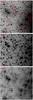 |
Fig. 8 1″ × 1″ E-ELT (top panel), TMT (middle panel), and JWST (bottom panel) images at 6re from the centre of the 1 Gyr old NSC at 2 Mpc. In the top panel the red circles show J = 28 mag stars, corresponding to the MSTO magnitude. |
4.2. IRIS@TMT
An example of a J-band IRIS simulated image is shown in Fig. 8. This image does not show significant difference with respect to the one obtained from MICADO simulations. we used Starfinder photometry obtained from the simulated image to derive a quantitative comparison between the performances of the IRIS and MICADO. The filter set of the two instruments is not the same, in particular IRIS will not be equipped with a I-band filter but a Z-band filter will be mounted. As the effective wavelength of I (λ = 0.90 μm) and Z (λ = 0.93 μm) bands are similar, we compare IRIS Z-band photometry with MICADO I-band one.
Figure 9 compares the CMDs obtained from the IRIS and MICADO simulated images. The magnitude limits and broadening of the evolutionary sequences in the two CMDs indicate that the photometric depth and accuracy of the two sets are comparable. The comparison of IRIS and MICADO photometric errors for MSTO stars is shown in the middle and lower panel of Fig. 9. The distributions of the differences between measured and input magnitudes are very similar for TMT and E-ELT photometry in both J and I (or Z) band. The only difference is that the TMT’s distributions are shifted towards negative values. This effect is very small (0.01−−0.02 mags) and is likely related to the higher contribution of stellar blends in the TMT photometric errors. The FWHM of MICADO PSF is in fact 5.1 mas in I-band and 6.3 mas in the J-band, while the FWHM of IRIS PSFs are 8.8 mas and 9.5 mas in Z and J-band respectively.
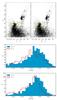 |
Fig. 9 Top panels: CMDs for stars in the 4 <r/re< 6 region of MICADO (left panel) and IRIS (right panel) simulated images. The green rectangle shows the region selected for the comparison of the photometric errors shown in the panels below. Middle panel: photometric errors for MSTO stars in 4 <r/re< 6 region of J-band MICADO and IRIS image. Lower panel: the same for MICADO J and IRIS Z-band images. MSTO have been selected in the box shown in the top panels. |
The photometric completeness of IRIS photometry is compared to the one of MICADO in Fig. 10. The two completeness curves are very similar. The J-band 50% completeness in MICADO photometry is found at magnitude ~0.2 mag fainter than in IRIS photometry. The same is found when comparing MICADO I-band with IRIS Z-band photometry.
On the one hand the E-ELT collecting area is larger than the one of TMT; on the other hand the MAORY PSF Strehl ratio is somewhat lower than the one foreseen for NFIRAOS (Ciliegi et al. 2012; Do et al. 2014). The two effects compensate each other and the performances of E-ELT and TMT imagers result to be very similar for the particular science application considered in this paper.
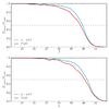 |
Fig. 10 Completeness of E-ELT and TMT I-band photometry. |
5. Summary and conclusions
In this paper we present simulated observations of NSCs in nearby galaxies. The simulated images were analysed using the Starfinder photometric package and the resulting CMDs were studied to assess the feasibility of the accurate study of the NSC stellar populations. For simplicity, we modelled NSCs with SSPs, but our results are applicable also to NSC originated from extended star-formation episodes; these complex stellar populations can be considered as the superposition of multiple SSPs. We constructed synthetic images adopting the parameters currently foreseen for the MICADO camera at E-ELT, exploring a number of cases with different age and distance of the NSC. We then proceeded with the photometric measurements of the images, the construction of the CMDs, and their analysis.
Our results are summarised in Fig. 11. We showed that E-ELT photometry could be used to age-date NSCs up to 10 Gyr in galaxies at 2 Mpc. Note, however, that the MSTO for the oldest stellar populations falls close to the detection limit and therefore the age estimates for the oldest stars will be uncertain. We evaluate these uncertainties using isochrones (Marigo et al. 2008) to derive a relation between cluster age and MSTO magnitude. For the 10 Gyr old cluster at 2 Mpc the photometric error is σJ = 0.29 mag for MSTO stars, corresponding to an age uncertainty σ [log (t)] = 0.10, –i.e.  Gyr. For galaxies at 4 Mpc the age of the NSC stellar population can be estimated with high accuracy only for young stellar populations. For oldest stellar populations the MSTO is detectable up to 4 Gyr. At this distance the MSTO of 4 Gyr-old stellar populations is detectable with a photometric uncertainty σJ = 0.35 mag, corresponding to σ [log (t)] = 0.12 –i.e.
  Gyr.
Gyr.
We can now extrapolate our results to galaxies located at different distances. In this paper we showed that E-ELT imaging can provide stellar photometry complete at a 50% level at J ≃ 30.0 mag. For stars 0.5 mag brighter than this the completeness reaches ~80% level. Using the relation between cluster age and MSTO magnitude, we calculated the age of SSPs whose MSTO is at J = 30.0 mag (and J = 29.5 mag) as a function of distance modulus. These relations are shown in Fig. 11 and we use them to extrapolate the results of our simulations. Stellar populations in the green area – below the J = 28.5 mag curve – will have a MSTO detectable above the ~80% completeness limit; for all these stellar populations the age will be therefore determined with a high reliability. In the case of stellar populations in the orange area, the photometric completeness for MSTO stars is estimated to be 50%−80%; in this case age measurements are expected to be affected by large uncertainties.
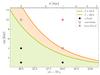 |
Fig. 11 Age of the oldest MSTO detectable as a function of the target distance. We show the results obtained adopting a detection magnitude limit of 30.0 and 29.5 in the J-band. These are the magnitudes corresponding to the 50% and 80% photometric completeness level. |
We finally investigated the possibility to obtain reliable photometry for resolved stellar populations in NSC with other next-generation instrumentation. We showed that the spatial resolution of the JWST is not sufficient to resolve nearby NSC into individual stars. Simulations of TMT images show that for our specific science case TMT and E-ELT performances are nearly equivalent and therefore the results of our analysis with the E-ELT can be applied also to TMT observations. To conclude, we showed that future ground-based 30 m class telescopes, equipped with advanced adaptive optics systems, will provide accurate photometric measurements of the resolved stars that will allow us to directly probe the formation and evolution of the stellar populations in NSC.
In the Cosmicflows-2 compilation of nearby galaxies with measured distance (Tully et al. 2013) there are 113 galaxies with distance between 2 and 4 Mpc. The estimate of the number of galaxies hosting a NSC is ~70% (Côté et al. 2006; Turner et al. 2012). It turns out therefore that the future facilities like E-ELT and TMT –that together are able to cover the whole sky– will provide the fundamental data to unveil the mechanisms of formation of the nuclear clusters of galaxies.
The typical size of a NSC (~3 pc) corresponds to  at 2 Mpc.
Acknowledgments
We acknowledge support of INAF and MIUR through the grant Progetto premiale T-REX. We warmly thank E. Diolaiti for the useful discussions. We thank S. Wright, T. Do, L. Wang and B. Ellerbroek for sharing their IRIS PSFs.
References
- Bekki, K. 2007, PASA, 24, 77 [NASA ADS] [CrossRef] [Google Scholar]
- Böker, T. 2010, in IAU Symp. 266, eds. R. de Grijs, & J. R. D. Lépine, 58 [Google Scholar]
- Böker, T., Laine, S., van der Marel, R. P., et al. 2002, AJ, 123, 1389 [NASA ADS] [CrossRef] [Google Scholar]
- Böker, T., Sarzi, M., McLaughlin, D. E., et al. 2004, AJ, 127, 105 [NASA ADS] [CrossRef] [Google Scholar]
- Capuzzo-Dolcetta, R., & Miocchi, P. 2008, ApJ, 681, 1136 [NASA ADS] [CrossRef] [Google Scholar]
- Ciliegi, P., Diolaiti, E., Baruffolo, A., et al. 2012, Mem. Soc. Astron. It., 83, 1151 [NASA ADS] [Google Scholar]
- Côté, P., Piatek, S., Ferrarese, L., et al. 2006, ApJS, 165, 57 [NASA ADS] [CrossRef] [MathSciNet] [Google Scholar]
- Davies, R., Ageorges, N., Barl, L., et al. 2010, in Ground-based and Airborne Instrumentation for Astronomy III, eds. I. S. McLean, S. K. Ramsay, & H. Takami, Proc. SPIE, 7735, 77352A [Google Scholar]
- Deep, A., Fiorentino, G., Tolstoy, E., et al. 2011, A&A, 531, A151 [NASA ADS] [CrossRef] [EDP Sciences] [Google Scholar]
- Diolaiti, E., Bendinelli, O., Bonaccini, D., et al. 2000, in Adaptive Optical Systems Technology, ed. P. L. Wizinowich, Proc. SPIE, 4007, 879 [Google Scholar]
- Diolaiti, E., Conan, J.-M., Foppiani, I., et al. 2010, in Adaptive Optics Systems II, eds. B. L. Ellerbroek, M. Hart, N. Hubin, & P. L. Wizinowich, Proc. SPIE, 7736, 77360R [Google Scholar]
- Do, T., Wright, S. A., Barth, A. J., et al. 2014, AJ, 147, 93 [NASA ADS] [CrossRef] [Google Scholar]
- Falomo, R., Fantinel, D., & Uslenghi, M. 2011, in Applications of Digital Image Processing XXXIV, ed. A. G. Tescher, Proc. SPIE, 8135, 813523 [Google Scholar]
- Ferrarese, L., Côté, P., Dalla Bontà, E., et al. 2006, ApJ, 644, L21 [NASA ADS] [CrossRef] [Google Scholar]
- Georgiev, I. Y., & Böker, T. 2014, MNRAS, 441, 3570 [NASA ADS] [CrossRef] [Google Scholar]
- Greene, T., Beichman, C., Gully-Santiago, M., et al. 2010, in Space Telescopes and Instrumentation 2010: Optical, Infrared, and Millimeter Wave, Proc. SPIE, 7731, 77310C [CrossRef] [Google Scholar]
- Greggio, L., & Renzini, A. 2011, Stellar Populations. A User Guide from Low to High Redshift (Wiley-VCH Verlag) [Google Scholar]
- Greggio, L., Falomo, R., Zaggia, S., Fantinel, D., & Uslenghi, M. 2012, PASP, 124, 653 [NASA ADS] [CrossRef] [Google Scholar]
- Larkin, J. E., Moore, A. M., Barton, E. J., et al. 2010, in Ground-based and Airborne Instrumentation for Astronomy III, eds. I. S. McLean, S. K. Ramsay, & H. Takami, Proc. SPIE, 7735, 773529 [Google Scholar]
- Marigo, P., Girardi, L., Bressan, A., et al. 2008, A&A, 482, 883 [NASA ADS] [CrossRef] [EDP Sciences] [Google Scholar]
- Neumayer, N., & Walcher, C. J. 2012, Adv. Astron., 2012, 709038 [NASA ADS] [Google Scholar]
- Paudel, S., Lisker, T., & Kuntschner, H. 2011, MNRAS, 413, 1764 [NASA ADS] [CrossRef] [Google Scholar]
- Rossa, J., van der Marel, R. P., Böker, T., et al. 2006, AJ, 132, 1074 [NASA ADS] [CrossRef] [Google Scholar]
- Schreiber, L., Diolaiti, E., Sollima, A., et al. 2012, in Adaptive Optics Systems III, eds. B. L. Ellerbroek, E. Marchetti, & J. P. Véran, Proc. SPIE, 8447, 84475V [Google Scholar]
- Schreiber, L., Greggio, L., Falomo, R., Fantinel, D., & Uslenghi, M. 2014, MNRAS, 437, 2966 [NASA ADS] [CrossRef] [Google Scholar]
- Scott, N., & Graham, A. W. 2013, ApJ, 763, 76 [NASA ADS] [CrossRef] [Google Scholar]
- Seth, A. C., Dalcanton, J. J., Hodge, P. W., & Debattista, V. P. 2006, AJ, 132, 2539 [NASA ADS] [CrossRef] [Google Scholar]
- Seth, A. C., Cappellari, M., Neumayer, N., et al. 2010, ApJ, 714, 713 [NASA ADS] [CrossRef] [Google Scholar]
- Tremaine, S. D., Ostriker, J. P., & Spitzer, Jr., L. 1975, ApJ, 196, 407 [NASA ADS] [CrossRef] [Google Scholar]
- Tully, R. B., Courtois, H. M., Dolphin, A. E., et al. 2013, AJ, 146, 86 [NASA ADS] [CrossRef] [Google Scholar]
- Turner, M. L., Côté, P., Ferrarese, L., et al. 2012, ApJS, 203, 5 [NASA ADS] [CrossRef] [Google Scholar]
- Walcher, C. J., Böker, T., Charlot, S., et al. 2006, ApJ, 649, 692 [NASA ADS] [CrossRef] [Google Scholar]
- Wehner, E. H., & Harris, W. E. 2006, ApJ, 644, L17 [NASA ADS] [CrossRef] [Google Scholar]
- Wright, S. A., Barton, E. J., Larkin, J. E., et al. 2010, in Ground-based and Airborne Instrumentation for Astronomy III, eds. I. S. McLean, S. K. Ramsay, & H. Takami, Proc. SPIE, 7735, 77357P [Google Scholar]
- Zoccali, M., Renzini, A., Ortolani, S., et al. 2003, A&A, 399, 931 [NASA ADS] [CrossRef] [EDP Sciences] [Google Scholar]
All Tables
Parameters of the SSPs used to simulate the NSCs: age, metallicity, total number of stars, I-band absolute magnitude, and total mass at birth.
All Figures
|
Fig. 1 Zoom of a 6″ × 3″ region of the J-band simulated MICADO@E-ELT image of the 1 Gyr old NSC located at 2 Mpc. The circles show the effective radius ( |
| In the text | |
|
Fig. 2 Colour–magnitude diagrams of different regions of the simulated stellar system obtained from MICADO simulations. The lines are the isochrones from Marigo et al. (2008) representative of the nuclear cluster stars. The red line is the MS and the RGB, while the blue line is the sequence of core He-burning stars, up to the first thermal pulse on the AGB. The upper-left sub-panels show the CMDs of the input stellar catalogues (NSC plus host galaxy main body). For clarity only stars in the inner 3re region are shown. |
| In the text | |
|
Fig. 3 Photometric errors in the simulation at 2 Mpc with the 1 Gyr old clusters in I and H-band. The first and third panels from the top show the σ+ (upper curves) and σ− (lower curves) values for each radial distance bin. The other two panels show the median error. The two vertical lines show the magnitude of the RC and the MSTO. |
| In the text | |
|
Fig. 4 Photometric errors for the simulation at 2 Mpc (upper panels) and 4 Mpc (lower panels) in the I and J bands for stars at magnitudes corresponding to the 1 Gyr MS turn-off and red-clump. The vertical line corresponds to the NSC tidal radius. |
| In the text | |
|
Fig. 5 I-band luminosity function of all input stars (grey) and of input stars position-matched with a source in the output catalogue (red). We also plotted the LF obtained from the measured magnitudes in the output catalogue (blue). The completeness function is shown by the green line and its scale is shown on the right-hand axis. The LFs are computed from stars with a radial distance between 3.5re and 4.5re in the images of the 1 Gyr old cluster at 2 Mpc. |
| In the text | |
|
Fig. 6 The 50% completeness magnitude as a function of the radial distance from the NSC centre. The vertical line is the NSC tidal radius. Results for the simulations with the 1 and 10 Gyr old clusters are shown in the upper and lower panels respectively. |
| In the text | |
|
Fig. 7 Statistical subtraction of host galaxy stellar members from the CMDs of NSC stellar populations. Only a few representative cases are shown. The upper panels show the CMDs in the target region. The CMDs of control field beyond the NSC tidal radius are shown in central panels. The resulting decontaminated CMDs are shown in the lower panels. In each panel we show stellar models from Marigo et al. (2008). The red line is the MS and the RGB, while the blue line is the sequence of core He-burning stars, up to the first AGB thermal pulse. |
| In the text | |
|
Fig. 8 1″ × 1″ E-ELT (top panel), TMT (middle panel), and JWST (bottom panel) images at 6re from the centre of the 1 Gyr old NSC at 2 Mpc. In the top panel the red circles show J = 28 mag stars, corresponding to the MSTO magnitude. |
| In the text | |
|
Fig. 9 Top panels: CMDs for stars in the 4 <r/re< 6 region of MICADO (left panel) and IRIS (right panel) simulated images. The green rectangle shows the region selected for the comparison of the photometric errors shown in the panels below. Middle panel: photometric errors for MSTO stars in 4 <r/re< 6 region of J-band MICADO and IRIS image. Lower panel: the same for MICADO J and IRIS Z-band images. MSTO have been selected in the box shown in the top panels. |
| In the text | |
|
Fig. 10 Completeness of E-ELT and TMT I-band photometry. |
| In the text | |
|
Fig. 11 Age of the oldest MSTO detectable as a function of the target distance. We show the results obtained adopting a detection magnitude limit of 30.0 and 29.5 in the J-band. These are the magnitudes corresponding to the 50% and 80% photometric completeness level. |
| In the text | |
Current usage metrics show cumulative count of Article Views (full-text article views including HTML views, PDF and ePub downloads, according to the available data) and Abstracts Views on Vision4Press platform.
Data correspond to usage on the plateform after 2015. The current usage metrics is available 48-96 hours after online publication and is updated daily on week days.
Initial download of the metrics may take a while.