| Issue |
A&A
Volume 568, August 2014
|
|
|---|---|---|
| Article Number | A93 | |
| Number of page(s) | 7 | |
| Section | Cosmology (including clusters of galaxies) | |
| DOI | https://doi.org/10.1051/0004-6361/201424062 | |
| Published online | 27 August 2014 | |
Galaxy clusters in presence of dark energy: a kinetic approach
1 Department of Physics, University of Rome “La Sapienza”, Piazzale Aldo Moro 2, 00185, Rome Italy
e-mail: This email address is being protected from spambots. You need JavaScript enabled to view it.
2 Space Research Institute, Russian Academy of Sciences, Moscow, Russia
3 National Research Nuclear University MEPhI, Moscow, Russia
e-mail: This email address is being protected from spambots. You need JavaScript enabled to view it.
4 Department of Physics, University of Rome “Tor Vergata”, via della Ricerca Scientifica 1, 00133 Rome, Italy
e-mail: This email address is being protected from spambots. You need JavaScript enabled to view it.
Received: 24 April 2014
Accepted: 9 July 2014
Abstract
Context. The external regions of galaxy clusters may be under strong influence of the dark energy, which was discovered by observations of supernovae Ia at redshift z< 1. The presence of the dark energy in the gravitational equilibrium equation, with the Einstein Λ term, balances the gravity, and extends the equilibrium configuration more in radius.
Aims. We investigate the features of the equilibrium configurations to analyse how the presence of the dark energy affects the density profiles and radial extension by specifying the conditions for which the gravitational equilibrium begins.
Methods. We derived the kinetic equation for an equilibrium configuration in presence of dark energy and solved the gravitational equilibrium equation by considering a Maxwell-Boltzmann distribution function with a cut-off in the framework of the Newtonian regime, because the observed velocities of galaxies inside a cluster are much lower than the velocity of light.
Results. The prevalence of dark energy effects on the gravity shows a wide region in the W0–ρΛ diagram where equilibrium solutions are not possible. In these particular conditions, the galaxies located in the external regions of a cluster can flow out, following the accelerating expansion of the Universe.
Key words: galaxies: clusters: general / dark energy / hydrodynamics
© ESO, 2014
1. Introduction
It was shown by Chernin (2001, 2008) that outer parts of galaxy clusters may be under strong influence of dark energy (DE), which was discovered by observations of supernovae (SN) Ia at redshift z ≤ 1 (Riess et al. 1998; Perlmutter et al. 1999) and in the spectrum of fluctuations of cosmic microwave background (CMB) radiation (see e.g. Spergel et al. 2003; Tegmark et al. 2004). To investigate these effects on the gravitational equilibrium of the clusters, solutions for polytropic configurations in presence of DE have been obtained by Balaguera-Antolínez et al. (2006, 2007) and Merafina et al. (2012). We here derive a Boltzmann-Vlasov kinetic equation in presence of DE and gravity in a Newtonian regime. The solutions generalize those obtained by Bisnovatyi-Kogan et al. (1993, 1998) for the kinetic equation without DE. The Newtonian approximation is chosen because the observed chaotic velocities of galaxies inside a cluster are much lower than the velocity of light.
The general relativistic solution in presence of DE can be applied for equilibrium configurations of point masses of some exotic particles that only interact gravitationally. In early stages of the Universe expansion, before and during the inflation stage, these particles may form gravitationally bound configurations that collapse during the inflation, when anti-gravity decreases. As a result of this collapse, such hypothetical objects may be transformed into primordial black holes that appear after the end of inflation. The relativistic kinetic equation and its solutions in presence of DE will be considered elsewhere.
2. Newtonian approximation in description of DE
The substance that is called now DE was first introduced by Einstein (1918) for a stationary universe in the form of the cosmological constant Λ during his unsuccessful attempts to construct a solution for a stationary universe. Shortly before this, de Sitter (1917) had shown that in presence of Λ the solution for an empty space describes an exponential expansion. Friedmann (1922, 1924) was the first to obtain exact solutions for the expanding universe that contained matter in presence of the cosmological constant Λ. Another exact solution for the metric in presence of Λ, around the gravitating point mass, was obtained by Carter (1973). This solution is a direct generalization of the Schwarzschild solution for a black hole (BH) in vacuum with a metric  (1)of the form
 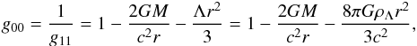 (2)where the density of DE ρΛ is connected with Λ as
  (3)A transition to the Newtonian limit, where DE is described by the anti-gravity force in vacuum, was made by Chernin (2008). In the limit of a weak gravity (v2 ≪ c2, GM/r ≪ c2) the metric coefficients are connected with a gravitational potential Φg as (Landau & Lifshitz 1962)
 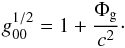 (4)Then, using the Eqs. (4) and (2) at Λ = 0, we obtain the expression for the Newtonian potential Φg and the Newtonian gravity force acting on the unit mass Fg
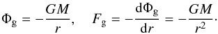 (5)For the Schwarzschild-de Sitter metric (2) we have in the Newtonian limit
  (6)In this way, the cosmological constant creates a repulsive (anti-gravity) force between a BH and a test particle in vacuum, which force increases linearly with a distance between them. The normalization of the potential here is chosen so that Φg = 0 at r = ∞, and ΦΛ = 0 at r = 0.
We now consider the equilibrium of a self-gravitating object in presence of DE. In general relativity the equations describing the equilibrium in a spherically symmetric configuration in vacuum (without DE) have been derived by Oppenheimer & Volkoff (1939)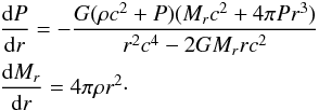 (7)
(7)
Here ρ, P are the total density and total pressure of the matter, and Mr is the total (gravitating) mass, including a gravitationally binding energy, inside a radius r in the Schwarzschild-like metric 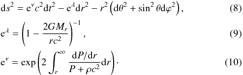
In presence of DE, ρ and P are represented as 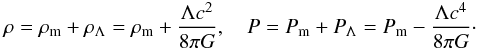 (11)We consider a Newtonian limit when
 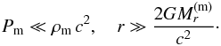 (12)Here we used a definition
  dr. In the Newtonian limit we have from Eq. (7)
 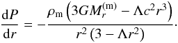 (13)We estimate the last term in the denominator. For an equilibrium configuration with a finite radius to exist, we need a positive sign of the numerator; from condition (12) we have
 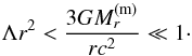 Therefore, in the denominator we have Λr2 ≪ 3 and we can neglet the term with Λ. In the Newtonian approximation, in presence of DE, we obtain the following equilibrium equation
 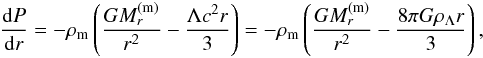 (14)with ρΛ given by definition (3), which was used without derivation by Merafina et al. (2012). On the other hand, we can write the Poisson equation for the gravity of the matter together with the hydrostatic equilibrium equation
 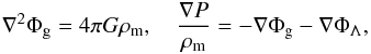 (15)and then, the potential created by DE in the vacuum, taking into account that P = Pm + PΛ, satisfies the Poisson equation
 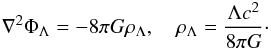 (16)This equation, together with the Poisson equation for the gravity of the matter fully describes a static gaseous equilibrium configuration in presence of DE. Similarly, we can write the hydrodynamic Euler equation in presence of DE as
 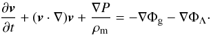 (17)
(17)
3. Kinetic equation for a self-gravitating cluster in presence of DE
The kinetic Boltzmann-Vlasov equation for a distribution function f of non-collisional gravitating points of equal mass m in spherical coordinates (r,θ,ϕ) is written as 
 (18)where, in presence of DE, we have Φ = Φg + ΦΛ. In a spherically symmetric stationary cluster, we have ∂Φ /∂t = 0 and Φ = Φ(r). Moreover, the kinetic Eq. (18) has four first integrals, written in Cartesian coordinates (x,y,z) as
  (19)In spherical coordinates, these integrals can be expressed by
  (20)where E and Li(i = x,y,z) are the energy and the projection of the angular momentum on the corresponding axis. From the last three integrals follows the conservation of the absolute value of the angular momentum L, written in the form
  (21)Then, the solution of the kinetic Eq. (18) is an arbitrary function of the first integrals (20). We restrict ourselves to an isotropic distribution function f(E). For a uniform DE, a normalization of its energy at r = ∞ is not possible, therefore we choose ΦΛ = 0 at r = 0 as the most convenient one (Merafina et al. 2012). Thus, from Eqs. (15), we have
  (22)Following Zel’dovich & Podurets (1965) and Bisnovatyi-Kogan et al. (1993, 1998), we consider a Maxwell-Boltzmann distribution function with a cut-off
 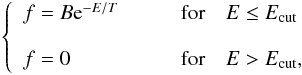 (23)where the cut-off energy Ecut is given by
  (24)and α is the so-called cut-off parameter, while T is the temperature in energy units. The total energy is
  (25)where the total potential Φ and the velocity v are given by
  (26)The constant B in the first of Eqs. (23) depends on the total potential Φ and therefore is different for each model. To consider a unique distribution function for all the equilibrium configurations, following Merafina & Ruffini (1989), we must choose a different normalization by introducing a new constant A connected with B through the following relation1
 (27)with ΦR the value of the total potential Φ at r = R. In this way, the expression of the distribution function (23) for E ≤ Ecut becomes
 ![Mathematical equation: \begin{eqnarray} f=A\,{\rm{exp}} \left[\frac{m\Phi_R}{T}-\frac{mv^2}{2T}-\frac{m}{T}\left(\Phi_{\rm g}- \frac{\Lambda c^2 r^2}{6}\right)\right] \cdot \label{eq21b} \end{eqnarray}](/articles/aa/full_html/2014/08/aa24062-14/aa24062-14-eq71.png) (28)The maximum kinetic energy ϵc is connected with the potential Φ by the relation
(28)The maximum kinetic energy ϵc is connected with the potential Φ by the relation 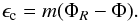 (29)Then the distribution function can be rewritten as
 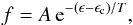 (30)where ϵ = mv2/ 2 is the kinetic energy of the single-point mass.
The Poisson Eq. (15) in a spherical symmetry applied to a gravitational field is given by 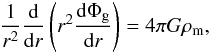 (31)with the boundary conditions Φg(0) = Φg0 and
  . The matter density can be expressed as
 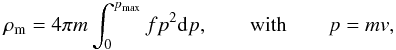 (32)where the expression of the maximum momentum pmax is given by
 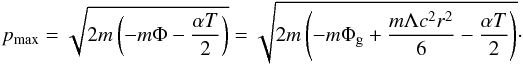 The cluster with a finite radius is possible only when the following condition is satisfied:
 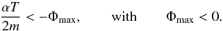 Then, by using the form of the distribution given in Eq. (30), we can finally rewrite the matter density as
 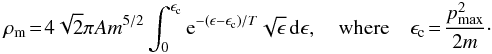 (33)Introducing dimensionless variables
 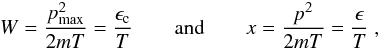 (34)we obtain W = m(ΦR − Φ) /T, and the expression of matter density ρm becomes
 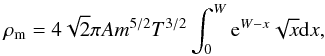 (35)where, as usual, at W = 0 we have ρm = 0, being Φ = ΦR.
From the Poisson Eq. (31) we can deduce the equation describing the structure of the Newtonian configurations in presence of DE by also considering the potential ΦΛ. In fact, inserting the expression of the gravitational potential Φg = Φ − ΦΛ into Eq. (31) and using Eq. (22), we obtain 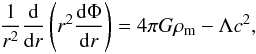 (36)where the potential Φ now includes all the contributions. Then, by considering the first relation in Eq. (11), the equilibrium equation becomes
 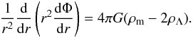 (37)Now, we have to consider the boundary conditions for the potential Φ with respect to the conditions given for the potential Φg in Eq. (31). Starting from Eq. (22), we can write
 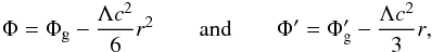 (38)and therefore, for r = 0, we have Φ(0) = Φg0 and
  .
.
To write the dimensionless form of the equilibrium equation, we can express the radial coordinate as  and, using the definition W = m(ΦR − Φ) /T, the equilibrium equation can be rewritten as
 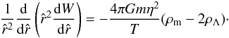 (39)In the same way, following Merafina & Ruffini (1989), we can introduce the expression of dimensionless densities by defining the following quantities
 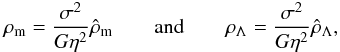 (40)where σ2 = 2T/m. Thus, the dimensionless form of the equilibrium equation will be given by
 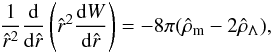 (41)with the boundary conditions W(0) = W0 and W′(0) = 0. Moreover, it is important to note that the relation
  must be satisfied at the centre of the equilibrium configuration to obtain the condition of initial decreasing density W′′(0) < 0. However, this is a necessary but not sufficient condition for the existence of the equilibrium solution, because the presence of the DE can enable conditions of increasing density (W′> 0) to be reached at other values of the radial coordinate.
We still need to define the expression of the dimensional quantity η. To derive the result, we can use the relations (35) and (11) for the densities ρm and ρΛ, respectively, and compare them with the definitions (40). We obtain 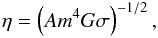 (42)with
 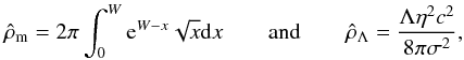 (43)where
  is given by the value of Λ. The total mass M(m) at radius R is given by
 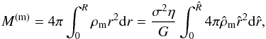 (44)where
 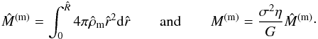 (45)Finally, to make the dependence of the dimensional quantities on the velocity σ explicit, we can introduce the quantity
 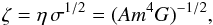 (46)and the dimensional quantities can be rewritten as
 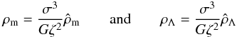 (47)and
 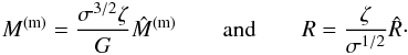 (48)Turning to the condition (24) on the energy Ecut, we can express the cut-off parameter α by using the condition at the edge of the configuration
  (49)Thus, because Φg(R) = −GM(m)/R and ΦΛ(R) = −Λc2R2/ 6, we obtain
 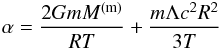 (50)and, finally, by using dimensionless quantities (47), (48) and relation (3), we have
 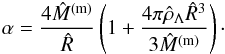 (51)For low values of the cut-off parameter α, maintaining a finite value of αT that corresponds to high values of the temperature T, the distribution function (23) may be taken as a constant (Bisnovatyi-Kogan et al. 1998). Then, the solutions only exist for low values of W0 and , assuming a more simplified form that converges to a limiting sequence. In the limit of W → 0, the dimensionless density ρm can be expressed as
 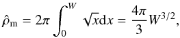 (52)whereas the equilibrium Eq. (41) becomes
 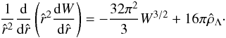 (53)Expressed in dimensional terms, the density can be written as
 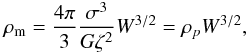 (54)where
 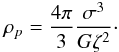 (55)Moreover, by imposing a change of radial coordinate from
  to y for which
  (56)the dimensionless equilibrium equation can be rewritten as
  (57)We can also substitute the density by using Eqs. (47) and (55) and finally obtain
  (58)which corresponds, if we take ρp = ρm0 and W ≡ θ, exactly to the equilibrium equation for a polytropic configuration with index n = 3/2 in presence of DE introduced by Merafina et al. (2012) in accordance with the dimensionless Emden variables and the initial conditions W(0) = θ(0) = 1 and W′(0) = θ′(0) = 0. Therefore, the polytropic configurations calculated by Merafina et al. (2012) in hydrostatic approach can be used to describe clusters of gravitating point masses with distribution function (28) with the energy cut-off (29), at low values of Λ and high values of T.
4. Numerical results
The dimensionless equilibrium Eq. (41) depends on two parameters: the gravitational potential at the centre of configurations W0 and , which determines the intensity of DE through the value of the cosmological constant Λ. Different values of these parameters give a two-dimensional family of equilibrium solutions. The set of solutions for  at different values of W0 was obtained by Bisnovatyi-Kogan et al. (1998).
We solved numerically the Poisson equation for gravitational equilibrium at different values of the two parameters (W0, ) mentioned above. First of all, we focused our attention on the matter density profiles ρm(r) of the equilibrium configurations; in detail, we investigated how they change for increasing values of the dimensionless DE density  at fixed values of the dimensionless gravitational potential W0. We chose three values of W0 and four values of , which are the basis of pairs of parameters (W0, ) that do not allow equilibrium solutions. This peculiarity is clearly represented in the matter density profiles shown in Figs. 1–3. For conciseness, we define the following quantitites in the figures:
  (59)and, therefore, the dimensionless quantities introduced in Eqs. (47) and (48) can be rewritten as
 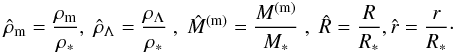 (60)For each value of the central potential W0 there is one value of the parameter after which the matter density profile does not converge to zero, but oscillates indefinitely. If we assert that the radius R of an equilibrium configuration is defined as the value of the radial coordinate r at which the matter density ρm(r) becomes zero, it is clear that every time this does not occur, we are unable to estimate the radial extension of the system. All configurations with a given value of W0 and that correspond to oscillating density profiles cannot be considered in gravitational equilibrium.
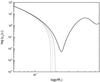 |
Fig. 1 Dimensionless matter density profiles for equilibrium configurations with W0 = 4 and |


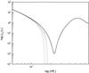 |
Fig. 2 Dimensionless matter density profiles for equilibrium configurations with W0 = 8 and |

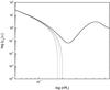 |
Fig. 3 Dimensionless matter density profiles for equilibrium configurations with W0 = 12 and |

Moreover, the calculation of the total radius R of an equilibrium configuration is strictly connected to the calculation related to the total mass M(m). Following Eq. (45) and expressed in terms of dimensionless quantities, the mass  within the radius is given by
  (61)As a consequence, the non-equilibrium solutions for which the total radius R cannot be defined do not even allow evaluating the total mass M(m) of the system.
Bisnovatyi-Kogan et al. (1998) found the set of solutions at Λ = 0 for  and
and  curves in the Newtonian case. These curves are shown in Figs. 4 and 5 (continuous line) together with the curves given for different values of (Λ ≠ 0). Analysing Fig. 4, when the parameter is different from zero, and for increasing values of this parameter, the curves are no longer continuous and the absolute maximum of the mass disappears. Within the interval
  , the curves present several branches (in the figure, only the branches for
  are shown to be able to clearly understand the different behaviours). Out of the interval
  the branches reduce to a unique curve and, in particular, for
  the curve becomes gradually shorter at increasing values of until it reaches the critical value
  , when the curve reduces to a unique point (we discuss this critical value below). It is clear that the unusual behaviour of the is related to the density profiles of the non-equilibrium solutions. To analyse Fig. 5, by considering Eq. (51), we can conclude that the parameter α is also connected to the values of the total radius
  and the mass
  . Consequently, it is easy to show that for non-equilibrium solutions it is not possible to calculate the cut-off parameter α. Therefore we can expect the existence of different branches of solutions here as well. Moreover, the behaviour of the curves at different values of extends the range of solutions at values of α higher than the critical value (α = 2.87) valid for Λ = 0 (Bisnovatyi-Kogan et al. 1998). As previously underlined, it is possible to distinguish several branches of solutions with a limiting value of α that changes in dependence of the value of . This limiting value, systematically higher than 2.87, increases at increasing values of until the absolute limiting value αlim ≃ 3.42.
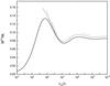 |
Fig. 4 Dimensionless mass as a function of the dimensionless central matter density for |
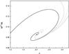 |
Fig. 5 Dimensionless mass as a function of the cut-off parameter α for |
The DE background in which all the bodies of the Universe are embedded produces the anti-gravity that changes their gravitational equilibrium, acting in contrast to the matter gravity. To establish when we have found configurations for which the presence of the DE can change the gravitational equilibrium, following Bisnovatyi-Kogan & Chernin (2012), we introduce the so-called zero gravity radius RΛ. This is a physical parameter that is defined as the distance from the centre of the system where the matter gravity and DE anti-gravity balance each other exactly. We consider the total force acting on the unit mass  (62)where, differently from Eq. (6), this relation is also valid within the matter and not only in the vacuum. Then, the total force F defined in Eq. (62) and, consequently, the acceleration, are both zero at a distance
 ![Mathematical equation: \begin{eqnarray} R_{\Lambda}=\left[\frac{3M^{\rm (m)}_{R_{\Lambda}}}{8\pi \rho_{\Lambda}}\right]^{1/3}, \label{eq38b} \end{eqnarray}](/articles/aa/full_html/2014/08/aa24062-14/aa24062-14-eq173.png) (63)where the zero-gravity radius depends on the total mass of the equilibrium configurations if R ≤ RΛ, while if the condition F = 0 is satisfied inside the configuration, we have no equilibrium, and the mass to consider is
(63)where the zero-gravity radius depends on the total mass of the equilibrium configurations if R ≤ RΛ, while if the condition F = 0 is satisfied inside the configuration, we have no equilibrium, and the mass to consider is  with r = RΛ.
This means that every cluster has its zero-gravity radius. This definition allows us to identify a gravitationally bound system only if it is enclosed within the sphere of radius RΛ, namely only if its total radius is smaller than its zero-gravity radius (R<RΛ). Galaxies in the external regions where r ≥ RΛ can flow out from the centre of the cluster under the action of the DE anti-gravity force.
In Fig. 6 we have represented the curve of the equilibrium configurations with R = RΛ, through the behaviour of W0 as a function of . In addition, we have also shown the curves that represent the families of equilibrium solutions at fixed values of α. When the value of W0 is kept constant and the value of is increased, we obtain one limiting value located on the curve after which it is no longer possible to obtain equilibrium solutions. Along this limiting curve, which separates two regions (solid line), the equilibrium configurations have the total radius exactly equal to the zero-gravity radius and the matter density profiles vanishing with a minimum in correspondence of the total radius R = RΛ. This enables defining the region on the right side of the figure in which no gravitational equilibrium can establish and no curves at constant α can lie, corresponding to configurations with matter density profiles that do not converge to zero. In contrast, in the region corresponding to the left side of the figure, we can assert that the force due to the presence of the DE, FΛ, is weaker than the force due to the gravity, Fg, and gravitational equilibrium can be achieved. In other words, speaking in terms of radial extension, the condition R ≤ RΛ is satisfied for each configuration belonging to this region, and the matter density profiles are regular and converging to zero in correspondence to the total radius R.
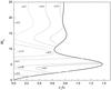 |
Fig. 6 Limiting curve of the equilibrium configurations with R = RΛ (solid line), expressed in terms of W0 as a funtion of |
Finally, from Eq. (63) we can see that the zero-gravity radius RΛ is inversely proportional to the DE density ρΛ. Therefore, by decreasing the value of the DE density, the zero-gravity radius increases until the condition RΛ → ∞ for ρΛ = 0. By considering the plane (W0-) of Fig. 6, the gravitational equilibrium is even achieved more easily and for more values of W0, when parameter is small. In particular, for  , the equilibrium solutions are possible for each value of W0, recovering the well-known results of Bisnovatyi-Kogan et al. (1998).
5. Conclusions
We have calculated the equilibrium configurations of Newtonian clusters with a truncated Maxwellian distribution function in presence of DE. All clusters that satisfy the condition R ≤ RΛ have a structural equilibrium and can be considered dynamically stable. On the other hand, there are conditions for which the effects of DE prevail on the gravity, and equilibrium cannot be reached. This occurs whenever the zero-gravity radius lies inside the configuration and divides the inner part, which is dominated by gravity, from the external part in which the expanding forces due to DE are prevalent.
Then we described the density distribution inside galaxy clusters by several phenomenological functions, some of which follow from numerical simulations (see Chernin et al. 2013). Qualitatively, the truncated Maxwellian distribution considered here is similar to the non-singular density distribution suggested by Chernin et al. (2013). It may be used for a more detailed study of the density and velocity distribution on the periphery of rich clusters, where the influence of DE is significant, and their comparison with observations.
The number density of the galaxies located in the outer part of a cluster is less relevant than those of the central region and, in general, these galaxies have smaller masses and lower luminosities in presence of an even weaker relaxation because of the low probability of encounters. Therefore, only the largest
telescopes should be used to search for galaxies in the external cluster regions. Furthermore, the most sensitive X-ray telescopes are needed to detect the hot gas in the low-density regions to reveal the possible outflow in presence of DE that was considered by Bisnovatyi-Kogan & Merafina (2013).
Finally, the evaluation of the parameters that characterize the clusters of galaxies suggests that these systems are collisionless. In fact, if we consider the relaxation time, we obtain higher values than the age of the Universe and, therefore, we can conclude that thermodynamical instabilities are irrelevant in the current evolution of the galaxy clusters. On the other hand, using well-known criteria for identifying the onset of thermodynamical instability (Bisnovatyi-Kogan & Merafina 2006), we can see that the critical point lies far from the first maximum mass of the curve with in Fig. 4, namely, at higher values of the central matter density, as well as in curves with  , which allows us to conclude that the larger part of the equilibrium configurations is thermodynamically stable.
Equation (27) is not arbitrary but justified by considerations of statistical mechanics, where E = constant along the motion of each single component of mass m and taking into account the presence of the chemical potential μ in the constant B, where μ + mΦ = const. along the radial coordinate r.
Acknowledgments
The work of G.S. Bisnovatyi-Kogan was partly supported by RFBR grant 11-02-00602, the RAN Program Formation and evolution of stars and galaxies, and Russian Federation President Grant for Support of Leading Scientific Schools NSh-5440.2012.2.
References
- Balaguera-Antolínez, A., Mota, D. F., & Nowakowski, M. 2006, Class. Quant. Grav., 23, 4497 [NASA ADS] [CrossRef] [Google Scholar]
- Balaguera-Antolínez, A., Mota, D. F., & Nowakowski, M. 2007, MNRAS, 382, 621 [NASA ADS] [CrossRef] [Google Scholar]
- Bisnovatyi-Kogan, G. S., & Chernin, A. D. 2012, Ap&SS, 338, 337 [NASA ADS] [CrossRef] [Google Scholar]
- Bisnovatyi-Kogan, G. S., & Merafina, M. 2006, ApJ, 653, 1445 [NASA ADS] [CrossRef] [Google Scholar]
- Bisnovatyi-Kogan, G. S., & Merafina, M. 2013, MNRAS, 434, 3628 [NASA ADS] [CrossRef] [Google Scholar]
- Bisnovatyi-Kogan, G. S., Merafina, M., Ruffini, R., & Vesperini, E. 1993, ApJ, 414, 187 [NASA ADS] [CrossRef] [Google Scholar]
- Bisnovatyi-Kogan, G. S., Merafina, M., Ruffini, R., & Vesperini, E. 1998, ApJ, 500, 217 [NASA ADS] [CrossRef] [Google Scholar]
- Carter, B. 1973, Black hole equilibrium states (Gordon & Breach) [Google Scholar]
- Chernin, A. D. 2001, Physics Uspekhi, 44, 1099 [Google Scholar]
- Chernin, A. D. 2008, Physics Uspekhi, 51, 253 [Google Scholar]
- Chernin, A. D., Bisnovatyi-Kogan, G. S., Teerikorpi, P., et al. 2013, A&A, 553, A101 [NASA ADS] [CrossRef] [EDP Sciences] [Google Scholar]
- de Sitter, W. 1917, Proc. Kon. Ned. Acad. Wet., 20, 229 [NASA ADS] [Google Scholar]
- Einstein, A. 1918, Sitzgsber. Preuss. Acad. Wiss., 1, 142 [Google Scholar]
- Friedmann, A. 1922, Z. Phys., 10, 377 [Google Scholar]
- Friedmann, A. 1924, Z. Phys., 21, 326 [Google Scholar]
- Landau, L. D., & Lifshitz, E. M. 1962, The classical theory of fields (Pergamon Press) [Google Scholar]
- Merafina, M., & Ruffini, R. 1989, A&A, 221, 4 [NASA ADS] [Google Scholar]
- Merafina, M., Bisnovatyi-Kogan, G. S., & Tarasov, S. O. 2012, A&A, 541, A84 [NASA ADS] [CrossRef] [EDP Sciences] [Google Scholar]
- Oppenheimer, J. R., & Volkoff, G. M. 1939, Phys. Rev., 55, 374 [NASA ADS] [CrossRef] [Google Scholar]
- Perlmutter, S., Aldering, G., Goldhaber, G., et al. 1999, ApJ, 517, 565 [NASA ADS] [CrossRef] [Google Scholar]
- Riess, A. G., Filippenko, A. V., Challis, P., et al. 1998, Observational Evidence from Supernovae for an Accelerating Universe and a Cosmological Constant, AJ, 116, 1009 [NASA ADS] [CrossRef] [Google Scholar]
- Spergel, D. N., Verde, L., & Peiris, H. V., et al. 2003, ApJS, 148, 175 [NASA ADS] [CrossRef] [Google Scholar]
- Tegmark, M., Strauss, M. A., Blanton, M. R., et al. 2004, Phys. Rev. D, 69, 103501 [CrossRef] [Google Scholar]
- Zel’dovich, Y. B., & Podurets, M. A. 1965, Astron. Zh., 42, 963 [NASA ADS] [Google Scholar]
All Figures
|
Fig. 1 Dimensionless matter density profiles for equilibrium configurations with W0 = 4 and |
| In the text | |
|
Fig. 2 Dimensionless matter density profiles for equilibrium configurations with W0 = 8 and |
| In the text | |
|
Fig. 3 Dimensionless matter density profiles for equilibrium configurations with W0 = 12 and |
| In the text | |
|
Fig. 4 Dimensionless mass as a function of the dimensionless central matter density for |
| In the text | |
|
Fig. 5 Dimensionless mass as a function of the cut-off parameter α for |
| In the text | |
|
Fig. 6 Limiting curve of the equilibrium configurations with R = RΛ (solid line), expressed in terms of W0 as a funtion of |
| In the text | |
Current usage metrics show cumulative count of Article Views (full-text article views including HTML views, PDF and ePub downloads, according to the available data) and Abstracts Views on Vision4Press platform.
Data correspond to usage on the plateform after 2015. The current usage metrics is available 48-96 hours after online publication and is updated daily on week days.
Initial download of the metrics may take a while.