| Issue |
A&A
Volume 568, August 2014
|
|
|---|---|---|
| Article Number | A64 | |
| Number of page(s) | 15 | |
| Section | Planets and planetary systems | |
| DOI | https://doi.org/10.1051/0004-6361/201322885 | |
| Published online | 15 August 2014 | |
Precise radial velocities of giant stars
VI. A possible 2:1 resonant planet pair around the K giant star η Ceti ⋆,⋆⋆
1
ZAH-Landessternwarte, Königstuhl 12, 69117
Heidelberg,
Germany
e-mail: This email address is being protected from spambots. You need JavaScript enabled to view it.
2
Department of Earth Sciences, The University of Hong
Kong, Pokfulam
Road, Hong Kong,
PR China
3
Department of Planetary Sciences and Lunar and Planetary
Laboratory, The University of Arizona, 1629 University Blvd., Tucson
AZ
85721,
USA
4
Department of Physics, The University of Hong Kong,
Pokfulman Road, Hong Kong, PR China
Received:
21
October
2013
Accepted:
20
June
2014
Abstract
We report the discovery of a new planetary system around the K giant η Cet (HIP 5364, HD 6805, HR 334) based on 118 high-precision optical radial velocities taken at Lick Observatory since July 2000. Since October 2011 an additional nine near-infrared Doppler measurements have been taken using the ESO CRIRES spectrograph (VLT, UT1). The visible data set shows two clear periodicities. Although we cannot completely rule out that the shorter period is due to rotational modulation of stellar features, the infrared data show the same variations as in the optical, which strongly supports that the variations are caused by two planets. Assuming the mass of η Cet to be 1.7 M⊙, the best edge-on coplanar dynamical fit to the data is consistent with two massive planets (mb sini = 2.6 ± 0.2 MJup, mc sini = 3.3 ± 0.2 MJup), with periods of Pb = 407 ± 3 days and Pc = 740 ± 5 days and eccentricities of eb = 0.12 ± 0.05 and ec = 0.08 ± 0.04. These mass and period ratios suggest possible strong interactions between the planets, and a dynamical test is mandatory. We tested a wide variety of edge-on coplanar and inclined planetary configurations for stability, which agree with the derived radial velocities. We find that for a coplanar configuration there are several isolated stable solutions and two well defined stability regions. In certain orbital configurations with moderate eb eccentricity, the planets can be effectively trapped in an anti-aligned 2:1 mean motion resonance that stabilizes the system. A much larger non-resonant stable region exists in low-eccentricity parameter space, although it appears to be much farther from the best fit than the 2:1 resonant region. In all other cases, the system is categorized as unstable or chaotic. Another conclusion from the coplanar inclined dynamical test is that the planets can be at most a factor of ~1.4 more massive than their suggested minimum masses. Assuming yet higher inclinations, and thus larger planetary masses, leads to instability in all cases. This stability constraint on the inclination excludes the possibility of two brown dwarfs, and strongly favors a planetary system.
Key words: techniques: radial velocities / planets and satellites: detection / planets and satellites: dynamical evolution and stability / planetary systems
Based on observations collected at Lick Observatory, University of California.
Based on observations collected at the European Southern Observatory, Chile, under program IDs 088.D-0132, 089.D-0186, 090.D-0155 and 091.D-0365.
© ESO, 2014
1. Introduction
Until May 2014, 387 known multiple planet systems were reported in the literature1, and their number is constantly growing. The first strong evidence for a multiple planetary system around a main-sequence star was reported by Butler et al. (1999), showing that together with the 4.6 day-period radial velocity signal of υ And (Butler et al. 1997), two more long-period, substellar companions can be derived from the Doppler curve. Later, a second Jupiter-mass planet was found to orbit the star 47 UMa (Fischer et al. 2002), and another one the G star HD 12661 (Fischer et al. 2003).
Interesting cases also include planets locked in mean motion resonance (MMR), such as the short-period 2:1 resonance pair around GJ 876 (Marcy et al. 2001), the 3:1 MMR planetary system around HD 60532 (Desort et al. 2008; Laskar & Correia 2009), or the 3:2 MMR system around HD 45364 (Correia et al. 2009). Follow-up radial velocity observations of well known planetary pairs showed evidence that some of them are actually part of higher-order multiple planetary systems. For example, two additional long-period planets are orbiting around GJ 876 (Rivera et al. 2010), and up to five planets are known to orbit 55 Cnc (Fischer et al. 2008). More recently, Lovis et al. (2011) announced a very dense, but still well-separated low-mass planetary system around the solar-type star HD 10180. Tuomi (2012) claimed that there might even be nine planets in this system, which would make it the most compact and populated extrasolar multiple system known to date.
Now, almost two decades since the announcement of 51 Peg b (Mayor & Queloz 1995), 55 multiple planetary systems have been found using high-precision Doppler spectroscopy2. Another 328 multiple planetary systems have been found with the transiting technique, the vast majority of them with the Kepler satellite. Techniques such as direct imaging (Marois et al. 2010) and micro-lensing (Gaudi et al. 2008) have also proven to be successful in detecting multiple extrasolar planetary systems.
The different techniques for detecting extrasolar planets and the combination between them shows that planetary systems appear to be very frequent in all kinds of stable configurations. Planetary systems are found to orbit around stars with different ages and spectral classes, including binaries (Lee et al. 2009) and even pulsars (Wolszczan & Frail 1992). Nevertheless, not many multiple planetary systems have been found around evolved giant stars so far. The multiple planetary systems appear to be a very small fraction of the planet occurrence statistics around evolved giants, which are dominated by single planetary systems. Up to date there is only one multiple planetary system candidate known around an evolved star (HD 102272, Niedzielski et al. 2009a), and two multiple systems consistent with brown dwarf mass companions around BD +20 2457 (Niedzielski et al. 2009b) and ν Oph (Quirrenbach et al. 2011; Sato et al. 2012).
In this paper we present evidence for two Jovian planets orbiting the K giant η Cet based on precise radial velocities. We also carry out an extensive stability analysis to demonstrate that the system is stable and to further constrain its parameters.
The outline of the paper is as follows: in Sect. 2 we introduce the stellar parameters for η Cet and describe our observations taken at Lick observatory and at the VLT. Section 3 describes the derivation of the spectroscopic orbital parameters. In Sect. 4 we explain our dynamical stability calculations, and in Sect. 5 we discuss the possible origin of the η Cet system and the population of planets around giants. Finally, we provide a summary in Sect. 6.
2. Observations and stellar characteristics
2.1. K giant star η Cet
η Cet (=HIP 5364, HD 6805, HR 334) is a bright (V = 3.46 mag), red giant clump star (B − V = 1.16). It is located at a distance of 37.99 ± 0.20 pc (van Leeuwen 2007) and flagged in the Hipparcos catalog as photometrically constant.
Luck & Challener (1995) proposed Teff = 4425 ± 100 K, derived from photometry, and log g = 2.65 ± 0.25 [ cm s-2 ] estimated from the ionization balance between Fe I and Fe II lines in the spectra. Luck & Challener (1995) derived [Fe/H] = 0.16 ± 0.05, and a mass of M = 1.3 ± 0.2 M⊙. The more recent study of η Cet by Berio et al. (2011) derived the stellar parameters as Teff = 4356 ± 55 K, luminosity L = 74.0 ± 3.7 L⊙, and the estimated radius as R = 15.10 ± 0.10 R⊙. Berio et al. (2011) roughly estimate the mass of η Cet to be M = 1.0−1.4 M⊙ by comparing its position in the Hertzsprung-Russell (HR) diagram with evolutionary tracks of solar metallicity.
By using a Lick template spectrum without iodine absorption cell lines, Hekker & Meléndez (2007) estimated the metallicity of η Cet to be [Fe/H] = 0.07 ± 0.1. Based on this metallicity and the observed position in the HR diagram, a trilinear interpolation in the evolutionary tracks and isochrones (Girardi et al. 2000) yields Teff = 4529 ± 19 K, log g = 2.36 ± 0.05 [ cm s-2 ], L = 77.1 ± 1.1 L⊙ and R = 14.3 ± 0.2 R⊙ (Reffert et al. 2014).
Stellar properties of η Cet.
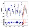 |
Fig. 1 Top panel: radial velocities measured at Lick Observatory (blue circles), along with error bars, covering about 11 years from July 2000 to October 2011. Two best fits to the Lick data are overplotted: a double-Keplerian fit (dot-dashed) and the best dynamical edge-on coplanar fit (solid line). The two fits are not consistent in later epochs because of the gravitational interactions considered in the dynamical model. Despite the large estimated errors, the data from CRIRES (red diamonds) seem to follow the best fit prediction from the dynamical fit. Bottom panel: no systematics are visible in the residuals. The remaining radial velocity scatter has a standard deviation of 15.9 m s-1, most likely caused by rapid solar – like p – mode oscillations. |
We determined the probability of η Cet to be on the red giant branch (RGB) or on the horizontal branch (HB) by generating 10 000 positions with (B − V, MV, [Fe/H]) consistent with the error bars on these quantities, and derived the stellar parameters via a comparison with interpolated evolutionary tracks. Our method for deriving stellar parameters for all G and K giant stars monitored at Lick Observatory, including η Cet, is described in more detail in Reffert et al. (2014).
Our results show that η Cet has a 70% probability to be on the RGB with a resulting mass of M = 1.7 ± 0.1 M⊙. If η Cet were on the HB, the mass would be M = 1.6 ± 0.2 M⊙. Here we simply use the mass with the highest probability. All stellar parameters are summarized in Table 1.
2.2. Lick data set
Doppler measurements for η Cet have been obtained since July 2000 as part of our precise (5–8 m s-1) Doppler survey of 373 very bright (V ≤ 6 mag) G and K giants. The program started in June 1999 using the 0.6 m Coudé Auxiliary Telescope (CAT) with the Hamilton Échelle Spectrograph at Lick Observatory. The original goal of the program was to study the intrinsic radial velocity variability in K giants, and to demonstrate that the low levels of stellar jitter make these stars a good choice for astrometric reference objects for the Space Interferometry Mission (SIM; Frink et al. 2001). However, the low amplitude of the intrinsic jitter of the selected K giants, together with the precise and regular observations, makes this survey sensitive to variations in the radial velocity that might be caused by extrasolar planets.
All observations at Lick Observatory have been taken with the iodine cell placed in the light path at the entrance of the spectrograph. This technique provides us with many narrow and very well defined iodine spectral lines, which are used as references, and it is known to yield precise Doppler shifts down to 3 m s-1 or even better for dwarf stars (Butler et al. 1996). The iodine method is not discussed in this paper; instead we refer to Marcy & Butler (1992),Valenti et al. (1995), and Butler et al. (1996), where more details about the technique and the data reduction can be found.
The wavelength coverage of the Hamilton spectra extends from 3755 to 9590 Å, with a resolution of R ≈ 60 000 in the wavelength range from 5000 to 5800 Å, where most of the iodine lines can be found and where the radial velocities are measured. The typical exposure time with the 0.6 m CAT is 450 s, which results in a signal-to-noise ratio (S/N) of about 100, reaching a radial velocity precision of better than 5 m s-1. The individual radial velocities are listed in Table 2, together with Julian dates and their formal errors.
2.3. CRIRES data set
Nine additional Doppler measurements for η Cet were taken between October 2011 and July 2013 with the pre-dispersed CRyogenic InfraRed Echelle Spectrograph (CRIRES) mounted at VLT UT1 (Antu), (Kaeufl et al. 2004). CRIRES has a resolving power of R ≈ 100000 when used with a 0.2′′ slit, covering a narrow wavelength region in the J,H,K,L or M infrared bands (960–5200 nm). Several studies have demonstrated that radial velocity measurements with precision between 10 and 35 m s-1 are possible with CRIRES. Seifahrt & Käufl (2008) reached a precision of ≈35 m s-1 when using reference spectra of a N2O gas cell, and Bean & Seifahrt (2009) even reached ≈10 m s-1 with an ammonia (NH3) gas-cell. Huélamo et al. (2008) and Figueira et al. (2010) showed that the achieved Doppler precision can be better than ≈25 m s-1 when using telluric absorption lines in the H band as reference spectra.
Motivated by these results, our strategy with CRIRES is to test the optical Doppler data with those from the near-IR regime for the objects in our G and K giants sample that clearly exhibit a periodicity consistent with one or more substellar companion(s). If the periodic Doppler signal were indeed caused by a planet, we would expect the near-IR radial velocities to follow the best-fit model derived from the optical spectra.
If the radial velocity variations in the optical and in the near-IR are not consistent, the reason may be either large stellar spots (Huélamo et al. 2008; Bean et al. 2010) or nonradial pulsations that will result in a different velocity amplitude at visible and infrared wavelengths (Percy et al. 2001). When stellar spots mimic a planetary signal, the contrast between the flux coming from the stellar photosphere and the flux coming from the cooler spot is higher at optical wavelengths and thus has a higher RV amplitude than the near-IR.
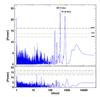 |
Fig. 2 Top panel: the periodogram of the measured radial velocities shows two highly significant peaks around 399 and 768 days, while the Kepler fit to the data reveals a best fit at periods around 403.5 and 751.9 days. Bottom panel: no significant peak is left in the periodogram of the residuals after removing the two periods from the Keplerian fit. |
For our observation with CRIRES we decided to adopt an observational setup similar to that successfully used by Figueira et al. (2010). We chose a wavelength setting in the H band (36/1/n), with a reference wavelength of λref = 1594.5 nm. This particular region was selected by inspecting the Arcturus near-IR spectral atlas from Hinkle et al. (1995) and searching for a good number of stellar as well as telluric lines. The selected spectral region is characterized by many deep and sharp atmospheric CO2 lines that take the role of an always available on-sky gas cell. To achieve the highest possible precision the spectrograph was used with a resolution of R = 100 000. To avoid RV errors related to a nonuniform illumination of the slit, the observations were made in NoAO mode (without adaptive optics), and nights with poor seeing conditions were requested.
Values for the central wavelengths of the telluric CO2 lines were obtained from the HITRAN database (Rothman et al. 1998), allowing us to construct an accurate wavelength solution for each detector frame. The wavelengths of the identified stellar spectral lines were taken from the Vienna Atomic Line Database (VALD; Kupka et al. 1999), based on the target’s Teff and log g.
Measured velocities for η Cet and derived errors.
Dark, flat, and nonlinearity corrections and the combination of the raw jittered frames in each nodding position were performed using the standard ESO CRIRES pipeline recipes. Later, the precise RV was obtained from a cross-correlation (Baranne et al. 1996) of the science spectra and the synthetic telluric and stellar mask; this was obtained for each frame and nodding position individually. We estimate the formal error of our CRIRES measurements to be on the order of ~40 m s-1, based on the rms dispersion values around the best fits for all good targets of our CRIRES sample. This error is probably overestimated, in particular, for the η Cet data set.
The full procedure of radial velocity extraction based on the cross-correlation method will be described in more detail in a follow-up paper (Trifonov et al., in prep.).
The CRIRES observations of η Cet were taken with an exposure time of 3 s, resulting in a S/N of ≈300. Our measured CRIRES radial velocities for η Cet are shown together with the data from Lick Observatory in Fig. 1, while the measured values are given in Table 2.
η Cet system best fits (Jacobi coordinates).
3. Orbital fit
Our measurements for η Cet, together with the formal errors and the best Keplerian and dynamical edge-on coplanar fits to the data, are shown in Fig. 1. We used the Systemic Console package (Meschiari et al. 2009) for the fitting.
A preliminary test for periodicities with a Lomb-Scargle periodogram shows two highly significant peaks around 399 and 768 days, suggesting two substellar companions around η Cet (see Fig. 2).
The sum of two Keplerian orbits provides a reasonable explanation of the η Cet radial velocity data (see Fig. 1). However, the relatively close planetary orbits and their derived minimum masses raise the question whether this planetary system suffers from sufficient gravitational perturbations between the bodies that might be detected in the observed data. For this reason we decided to use Newtonian dynamical fits, applying the Gragg-Bulirsch-Stoer integration method (B-SM: Press et al. 1992), built into Systemic. In this case gravitational perturbations that occur between the planets are taken into account in the model.
We used the simulated annealing method (SA: Press et al.
1992) to determine whether there is more than one
 local minimum in the data. When the global
minimum is found, the derived Jacobi orbital elements from the dynamical fit are the masses
of the planets mb,c, the periods
Pb,c, eccentricities
eb,c, longitudes of
periastron ϖb,c, and the mean
anomaly Mb,c (b always denotes the inner
planet and c
the outer planet). To explore the statistical and dynamical properties of the fits around
the best fit, we adopted the systematic grid-search techniques coupled with dynamical
fitting. This technique is fully described for the HD 82943 two-planet system (Tan et al. 2013).
local minimum in the data. When the global
minimum is found, the derived Jacobi orbital elements from the dynamical fit are the masses
of the planets mb,c, the periods
Pb,c, eccentricities
eb,c, longitudes of
periastron ϖb,c, and the mean
anomaly Mb,c (b always denotes the inner
planet and c
the outer planet). To explore the statistical and dynamical properties of the fits around
the best fit, we adopted the systematic grid-search techniques coupled with dynamical
fitting. This technique is fully described for the HD 82943 two-planet system (Tan et al. 2013).
It is important to note that a good fit means that the
solution is close to one. In our case the
best edge-on coplanar fit has  (see Sect. 3.1) for 118 radial velocity data points, meaning that the data are scattered
around the fit, and this can indeed be seen in Fig. 1.
The reason for that is additional radial velocity stellar jitter of about ~15 m s-1 that is not taken into account
in the weights of each data point.
(see Sect. 3.1) for 118 radial velocity data points, meaning that the data are scattered
around the fit, and this can indeed be seen in Fig. 1.
The reason for that is additional radial velocity stellar jitter of about ~15 m s-1 that is not taken into account
in the weights of each data point.
This jitter value was determined directly as the rms of the residual deviation around the model. In fact, this value is close to the bottom envelope of the points in Fig. 3 for η Cet’s color index (B − V = 1.16), which is likely the lowest jitter for η Cet. Based on the long period of our study and the large sample of stars with similar physical characteristics, we found that the intrinsic stellar jitter is clearly correlated with the color index B – V of the stars. and its value for η Cet is typical for other K2 III giants in our Lick sample (see Fig. 3). For η Cet we estimated an expected jitter value of 25 m s-1 (see Fig. 3), which is higher than the jitter estimated from the rms of the fit. It is also known that late G giants (Frandsen et al. 2002; De Ridder et al. 2006) and K giants (Barban et al. 2004; Zechmeister et al. 2008) exhibit rapid solar-like p-mode oscillations, much more rapid than the typical time sampling of our observations, which appear as scatter in our data. Using the scaling relation from Kjeldsen & Bedding (1995, 2011), the stellar oscillations for η Cet are estimated to have a period of ~0.4 days and an amplitude of ~11 m s-1, which again agrees well with η Cet’s RV scatter level around the fit.
We re-assessed the by quadratically adding the stellar jitter
to the formal observational errors (3–5 m s-1) for each radial velocity data point, which scaled down
the of the best fit close to unity. For our
edge-on coplanar case is scaled down to
 . We provide both: the unscaled
value together with the derived stellar
jitter and the value where the average stellar jitter
derived above is taken into account.
. We provide both: the unscaled
value together with the derived stellar
jitter and the value where the average stellar jitter
derived above is taken into account.
We estimated the error of the derived orbital parameters using two independent methods available as part of the Console: bootstrap synthetic data-refitting and MCMC statistics, which runs multiple MCMC chains in parallel with an adaptive step length. Both estimators gave similar formal errors for the orbital parameters. However, the MCMC statistics has been proven to provide better estimates of planetary orbit uncertainties than the more robust bootstrap algorithm (e.g. Ford 2005). Therefore, we will use only the MCMC results in this paper.
The nine near-IR Doppler points from CRIRES are overplotted in Fig. 1, but were not used for fitting. We did not consider the CRIRES data because of their large uncertainties and the negligible total weight to the fit, compared with the Lick data. Another complication is the radial velocity offset between the two data sets, which introduces an additional parameter in the χ2 fitting procedure. Nevertheless, the CRIRES data points agree well with the Newtonian fit predictions based on the optical data (see Fig. 1), providing strong evidence for the two-planet hypothesis.
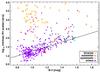 |
Fig. 3 Intrinsic RV scatter observed in our sample of 373 K giants versus B – V color. A clear trend is visible in the sense that redder stars without companions (circles) have larger intrinsic RV variations. A number of stars lie above the almost linear relation between color and the logarithm of the scatter. These stars have clearly periodic RVs, which indicates that they harbor substellar or stellar companions. Stars with non-periodic, but still systematic radial velocities are indicated with green crosses. The RV scatter of ~15 m s-1, for η Cet (red star) derived as the rms around the orbital fit, is lower than the 25 m s-1 derived from the linear trend at the star’s color index. |
 |
Fig. 4 Semi-major axes evolution of the best dynamical fits. Left: the edge-on coplanar fit remains stable in a 2:1 MMR only for 17 000 years, when the system starts to show chaotic behavior and eventually ejects the outer planet. The best inclined coplanar (middle) and mutually inclined (right) fits fail to preserve stability even on very short timescales. |
3.1. Formally best edge-on coplanar fit
Assuming an edge-on, co-planar planetary system (ib,c =
90°), the global minimum has (1.001 with jitter), which constitutes a
significant improvement from the best two-Keplerian fit with
 (1.17 with jitter). This
improvement indicates that the strong
interaction between the two planetary companions is visible in the radial velocity signal
even on short timescales. The derived planetary masses are mbsinib
= 2.5 MJup and mcsinic
= 3.3 MJup, with periods of Pb =
407.5 days and Pc = 739.9 days. The
eccentricities are moderate (eb = 0.12 and
ec = 0.08), and the
longitudes of periastron suggest an anti-aligned configuration with ϖb =
245.1° and ϖc = 68.2°, that is,
ϖb −
ϖc ≈ 180°. Orbital
parameters for both planets, together with their formal uncertainties, are summarized in
Table 3.
(1.17 with jitter). This
improvement indicates that the strong
interaction between the two planetary companions is visible in the radial velocity signal
even on short timescales. The derived planetary masses are mbsinib
= 2.5 MJup and mcsinic
= 3.3 MJup, with periods of Pb =
407.5 days and Pc = 739.9 days. The
eccentricities are moderate (eb = 0.12 and
ec = 0.08), and the
longitudes of periastron suggest an anti-aligned configuration with ϖb =
245.1° and ϖc = 68.2°, that is,
ϖb −
ϖc ≈ 180°. Orbital
parameters for both planets, together with their formal uncertainties, are summarized in
Table 3.
Dynamical simulations, however, indicate that this fit is stable only for ≲17 000 yr. After the start of the integrations, the planetary semi-major axes evolution shows a very high perturbation rate with a constant amplitude. Although the initially derived periods do not suggest any low-order MMR, the average planetary periods appear to be in a ratio of 2:1 during the first 17 000 years of orbital evolution, before the system becomes chaotic and eventually ejects the outer companion. This indicates that within the orbital parameter errors, the system might be in a long-term stable 2:1 MMR. Such stable edge-on cases are discussed in Sects. 4.2 and 4.3. The evolution of the planetary semi-major axes for this best-fit configuration is illustrated in Fig. 4.
3.2. Formally best inclined fits
We also tested whether our best dynamical fit improved significantly by allowing the inclinations with respect to the observer’s line of sight (LOS), and the longitudes of the ascending nodes of the planets to be ib,c ≠ 90° and ΔΩb,c = Ωb − Ωc ≠ 0, respectively.
The impact of the LOS inclinations on the fits mainly manifests itself through the
derived planetary masses. The mass function is given by
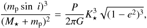 (1)where mp is the
planetary mass, M⋆ the stellar mass,
and G is the
universal gravitational constant, while the other parameters come from the orbital model:
period (P),
eccentricity (e), and radial velocity amplitude (K⋆). It is easy to see
that if we take sin i ≠
1 (i ≠
90°), the mass of the planet must increase to satisfy the right side of
the equation. However, we note that this general expression is valid only for the simple
case of one planet orbiting a star. Hierarchical two-planet systems and the dependence of
the minimum planetary mass on the inclination are better described in Jacobian
coordinates. For more details, we refer to the formalism given in Lee & Peale (2002).
(1)where mp is the
planetary mass, M⋆ the stellar mass,
and G is the
universal gravitational constant, while the other parameters come from the orbital model:
period (P),
eccentricity (e), and radial velocity amplitude (K⋆). It is easy to see
that if we take sin i ≠
1 (i ≠
90°), the mass of the planet must increase to satisfy the right side of
the equation. However, we note that this general expression is valid only for the simple
case of one planet orbiting a star. Hierarchical two-planet systems and the dependence of
the minimum planetary mass on the inclination are better described in Jacobian
coordinates. For more details, we refer to the formalism given in Lee & Peale (2002).
We separated the inclined fits in two different sets, depending on whether the planets are strictly in a coplanar configuration (yet inclined with respect to the LOS), or if an additional mutual inclination angle between the planetary orbits is allowed (i.e., ib − ic ≠ 0° and Ωb − Ωc ≠ 0°).
For the inclined co-planar test we set ib = ic, but sinib,c≤ 1, and we fixed the longitudes of
ascending nodes to Ωb = Ωc =
0°. In the second test the
inclinations of both planets were fitted as independent parameters, allowing mutually
inclined orbits. However, ib and
ic were restricted to
not exceed the sinib,c = 0.42
(ib,c = 90° ± 65°)
limit, where the planetary masses will become very large. Moreover, as discussed in Laughlin et al. (2002) and in Bean & Seifahrt (2009), the mutual inclination (Φb,c) of two orbits
depends not only on the inclinations ib and ic, but also on the
longitudes of the ascending nodes Ωb and Ωc:
 (2)The longitudes of the ascending node,
Ωb and Ωc, are not
restricted and thus can vary in the range from 0 to 2π. The broad range of
ib,c and
Ωb,c might lead to very high mutual
inclinations, but in general Φb,c was restricted
to 50°, although this limit
was never reached by the fitting algorithm.
(2)The longitudes of the ascending node,
Ωb and Ωc, are not
restricted and thus can vary in the range from 0 to 2π. The broad range of
ib,c and
Ωb,c might lead to very high mutual
inclinations, but in general Φb,c was restricted
to 50°, although this limit
was never reached by the fitting algorithm.
For the coplanar inclined case, the minimum appears to be
 , while adding the same stellar jitter as
above to the data used for the coplanar fit gives
, while adding the same stellar jitter as
above to the data used for the coplanar fit gives  . Both planets have orbits with relatively
high inclinations with respect to the LOS (ib,c = 35.5°). The
planetary masses are mb = 3.85
MJup and mc = 5.52
MJup, and the planetary periods are
closer to the 2:1 ratio: Pb = 396.8 days and
Pc = 767.1 days.
. Both planets have orbits with relatively
high inclinations with respect to the LOS (ib,c = 35.5°). The
planetary masses are mb = 3.85
MJup and mc = 5.52
MJup, and the planetary periods are
closer to the 2:1 ratio: Pb = 396.8 days and
Pc = 767.1 days.
The derived mutually inclined best fit has  , ( = 0.95). This fit also has high planetary
inclinations and thus the planetary masses are much more massive: mb = 5.50
MJup and mc = 7.74
MJup, while the periods are
Pb = 404.4 days and
Pc = 748.2 days.
Orbital parameters and the associated errors for the inclined fits are summarized in Table
3. An F-test shows that the probability that the
three additional fitting parameters significantly improve the model is ~90%.
, ( = 0.95). This fit also has high planetary
inclinations and thus the planetary masses are much more massive: mb = 5.50
MJup and mc = 7.74
MJup, while the periods are
Pb = 404.4 days and
Pc = 748.2 days.
Orbital parameters and the associated errors for the inclined fits are summarized in Table
3. An F-test shows that the probability that the
three additional fitting parameters significantly improve the model is ~90%.
Dynamical simulations based on the inclined fits show that these solutions cannot even preserve stability on very short timescales. The large planetary masses in those cases and the higher interaction rate make these systems much more fragile than the edge-on coplanar system. The best inclined co-planar fit appears to be very unstable and leads to planetary collision in less than 1600 years. The best mutually inclined fit is chaotic from the very beginning of the integrations. During the simulations the planets exchange their positions in the system until the outer planet is ejected after ~9000 years. The semi-major axes evolution for those systems is illustrated in Fig. 4.
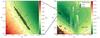 |
Fig. 5 Right: edge-on coplanar |
4. Stability tests
4.1. Numerical setup
For testing the stability of the η Cet planetary system we used the Mercury
N-body simulator (Chambers 1999), and the SyMBA integrator (Duncan et al. 1998). Both packages have been designed to calculate the
orbital evolution of objects moving in the gravitational field of a much more massive
central body, as in the case of extrasolar planetary systems. We used Mercury
as our primary program and SyMBA to double-check the obtained
results. All dynamical simulations were run using the hybrid sympletic/Bulirsch-Stoer
algorithm, which is able to compute close encounters between the planets if they occur
during the orbital evolution. The orbital parameters for the integrations are taken
directly from high-density grids (see Sects. 4.2, 4.3, 4.4 and 4.5) (~120 000 fits). Our goal is to check
the permitted stability regions for the η Cet planetary system and to constrain the orbital
parameters by requiring stability.
The orbital parameter input for the integrations are in astrocentric
format: mean anomaly M, semi-major axis a, eccentricity
e, argument
of periastron ω, orbital inclination i, longitude of the
ascending node Ω, and absolute
planetary mass derived from fit (dependent on the LOS inclination). The argument of
periastron is ω =
ϖ – Ω, and for an edge-on or co-planar configuration Ω is undefined and thus ω = ϖ.
From the orbital period P and assuming mb,csin
ib.c ≪
M⋆, the semi-major axes
ab,c are calculated
from the general form for the two-body problem:
 (3)Another input parameter is the Hill
radius, which indicates the maximum distance from the body that constitutes a
close encounter. A Hill radius approximation (Hamilton
& Burns 1992) is calculated from
(3)Another input parameter is the Hill
radius, which indicates the maximum distance from the body that constitutes a
close encounter. A Hill radius approximation (Hamilton
& Burns 1992) is calculated from
 (4)All simulations were started from JD =
2 451 745.994, the epoch when the first RV observation of η Cet was taken, and then
integrated for 105
years. This timescale was chosen carefully to minimize CPU resources, while still allowing
a detailed study of the system’s evolution and stability. When a test system survived this
period, we tested whether the system remains stable over a longer period of time by
extending the integration time to 108 years for the edge-on coplanar fits (Sect. 4.2), and to 2 × 10⁶ years for inclined configurations (Sects. 4.3 and 4.4). On
the other hand, the simulations were interrupted in case of collisions between the bodies
involved in the test, or ejection of one of the planets. The typical time step we used for
each dynamical integration was equal to eight days, while the output interval from the
integrations was set to one year. We defined an ejection as one of the planet’s semi-major
axes exceeding 5 AU during the integration time.
(4)All simulations were started from JD =
2 451 745.994, the epoch when the first RV observation of η Cet was taken, and then
integrated for 105
years. This timescale was chosen carefully to minimize CPU resources, while still allowing
a detailed study of the system’s evolution and stability. When a test system survived this
period, we tested whether the system remains stable over a longer period of time by
extending the integration time to 108 years for the edge-on coplanar fits (Sect. 4.2), and to 2 × 10⁶ years for inclined configurations (Sects. 4.3 and 4.4). On
the other hand, the simulations were interrupted in case of collisions between the bodies
involved in the test, or ejection of one of the planets. The typical time step we used for
each dynamical integration was equal to eight days, while the output interval from the
integrations was set to one year. We defined an ejection as one of the planet’s semi-major
axes exceeding 5 AU during the integration time.
In some cases none of the planets was ejected from the system and no planet-planet or planet-star collisions occurred, but because of close encounters, their eccentricities became very high and the semi-major axes showed single or multiple time planetary scattering to a different semi-major axis within the 5 AU limit. These systems showed an unpredictable behavior, and we classified them as chaotic, even though they may not satisfy the technical definition of chaos.
We defined a system to be stable if the planetary semi-major axes remained within 0.2 AU from the semi-major axes values at the beginning of the simulation during the maximum integration time. This stability criterion provided us with a very fast and accurate estimate of the dynamical behavior of the system, and clearly distinguished the stable from the chaotic and the unstable configurations. In this paper we do not discuss the scattering (chaotic) configurations, but instead focus on the configurations that we qualify as stable.
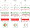 |
Fig. 6 Evolution of the orbital parameters for three different fits, stable for at least 108 years. The best 2:1 MMR fit (left panels), the best stable fit from the low-eccentricity region (middle panels), and the fit with the most circular orbits (right panels). In the 2:1 MMR fit the gravitational perturbation between the planets is much larger than in the other two cases. It is easy to see that eccentricities for given epochs can be much larger than their values at the initial epoch of the integration. For convenience the evolution of the semi-major axes, eccentricities, the resonant angles (third row) and the Δωb,c are given for 500 and 105 years, respectively. The bottom row gives the orbital precession region, the sum of orbits for each integration output. |
4.2. Two-planet edge-on coplanar system
The instability of the best fits motivated us to start a high-density
grid search to understand the possible
sets of orbital configurations for the η Cet planetary system. To construct these grids we
used only scaled fits with stellar jitter quadratically
added, so that is close to unity. Later, we tested each
individual set for stability, transforming these grids to effective stability maps.
In the edge-on coplanar two dimensional grid we varied the eccentricities of the planets
from eb,c = 0.001 (to have
access to ϖb,c) to 0.251 with
steps of 0.005 (50 × 50
dynamical fits), while the remaining orbital parameters in the model (mb,csin
ib,c, Pb,c, Mb,c, ϖb,c and the RV offset)
were fitted until the best possible solution to the data was achieved. The resulting
grid is smoothed with bilinear
interpolation between each grid pixel, and 1, 2 and 3σ confidence levels (based
on  from the minimum) are shown (see Fig.
5). The grid itself shows that very reasonable
fits can be found in a broad range of
eccentricities, with a tendency toward lower values in higher and moderate
eccentricities, and slightly poorer fits are found for the near-circular orbits. However,
our dynamical test of the edge-on coplanar grid illustrated in Fig. 5 shows that the vast majority of these fits are unstable. The
exceptions are a few isolated stable and chaotic cases, a large stable region at lower
eccentricities, and a narrow stable island with moderate eb, located about
1σ away
from the global minimum.
from the minimum) are shown (see Fig.
5). The grid itself shows that very reasonable
fits can be found in a broad range of
eccentricities, with a tendency toward lower values in higher and moderate
eccentricities, and slightly poorer fits are found for the near-circular orbits. However,
our dynamical test of the edge-on coplanar grid illustrated in Fig. 5 shows that the vast majority of these fits are unstable. The
exceptions are a few isolated stable and chaotic cases, a large stable region at lower
eccentricities, and a narrow stable island with moderate eb, located about
1σ away
from the global minimum.
4.2.1. Stable near-circular configuration
It is not surprising that the planetary system has better chances to survive with near circular orbits. In these configurations, the bodies might interact gravitationally, but at any epoch they will be distant enough to not exhibit close encounters. By performing direct long-term N-body integrations, we conclude that the individual fits in the low-eccentricity region are stable for at least 108 years, and none of them is involved in low-order MMR. Instead, the average period ratio of the stable fits in this region is between 1.8 for the very circular fits and 1.88 at the border of the stable region. This range of ratios is far away from the 2:1 MMR, but could be close to a high-order MMR like 9:5, 11:6, 13:7, or even 15:8. However, we did not study these possible high-order resonances, and we assume that if not in 2:1 MMR, then the planetary system is likely dominated by secular interactions.
The right column of Fig. 6 shows the dynamical
evolution of the most circular fit from Fig. 5 with
 ,
(
,
( ), mbsinib
= 2.4 MJup, mcsinic
= 3.2 MJup, ab =
1.28 AU, ac = 1.94 AU. We
started simulations with eb,c = 0.001, and
the gravitational interactions forced the eccentricities to oscillate very rapidly
between 0.00 and 0.06 for η Cet b, and between 0.00 to 0.03 for
η Cet c.
The arguments of periastron ωb and
ωc circulate between
0 and 360°, but the secular
resonant angle Δωb,c =
ωc −
ωb, while
circulating, seems to spend more time around 180° (anti-aligned). Within the stable
near-circular region, the gravitational perturbations between the planets have lower
amplitudes in the case of the most circular orbits than other stable fits with higher
initial eccentricities (and smaller ).
), mbsinib
= 2.4 MJup, mcsinic
= 3.2 MJup, ab =
1.28 AU, ac = 1.94 AU. We
started simulations with eb,c = 0.001, and
the gravitational interactions forced the eccentricities to oscillate very rapidly
between 0.00 and 0.06 for η Cet b, and between 0.00 to 0.03 for
η Cet c.
The arguments of periastron ωb and
ωc circulate between
0 and 360°, but the secular
resonant angle Δωb,c =
ωc −
ωb, while
circulating, seems to spend more time around 180° (anti-aligned). Within the stable
near-circular region, the gravitational perturbations between the planets have lower
amplitudes in the case of the most circular orbits than other stable fits with higher
initial eccentricities (and smaller ).
The middle column of Fig. 6 illustrates the best
fit within the low-eccentricity stable
region with = 13.03
( ) and initial orbital parameters of
mbsinib
= 2.4 MJup, mcsinic
= 3.2 MJup, ab =
1.28 AU, ac = 1.93 AU,
eb = 0.06, and
ec = 0.001. The mean
value of Δωb,c is again
around 180°, while the
amplitude is ≈±90°.
Immediately after the start of the integrations ec has increased from
close to 0.00 to 0.07, and oscillates in this range during the dynamical test, while
eb oscillates from
0.05 to 0.11. In particular, the highest value for eb is very interesting
because, as can be seen from Fig. 5, starting
integrations with 0.08
<eb< 0.11 in
the initial epoch yields unstable solutions. The numerical stability of the system
appears to be strongly dependent on the initial conditions that are passed to the
integrator. For different epochs the gravitational perturbations in the system would
yield different orbital parameters than derived from the fit, and starting the
integrations from an epoch forward or backward in time where eb or ec are larger than the
eb,c = 0.08 limit
might be perfectly stable.
) and initial orbital parameters of
mbsinib
= 2.4 MJup, mcsinic
= 3.2 MJup, ab =
1.28 AU, ac = 1.93 AU,
eb = 0.06, and
ec = 0.001. The mean
value of Δωb,c is again
around 180°, while the
amplitude is ≈±90°.
Immediately after the start of the integrations ec has increased from
close to 0.00 to 0.07, and oscillates in this range during the dynamical test, while
eb oscillates from
0.05 to 0.11. In particular, the highest value for eb is very interesting
because, as can be seen from Fig. 5, starting
integrations with 0.08
<eb< 0.11 in
the initial epoch yields unstable solutions. The numerical stability of the system
appears to be strongly dependent on the initial conditions that are passed to the
integrator. For different epochs the gravitational perturbations in the system would
yield different orbital parameters than derived from the fit, and starting the
integrations from an epoch forward or backward in time where eb or ec are larger than the
eb,c = 0.08 limit
might be perfectly stable.
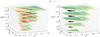 |
Fig. 7 Coplanar inclined grids illustrate the stability dependence on mb,csinib,c. Color maps are the same as in Fig. 5, with the difference that for clarity, only the stable regions are shown (black). The top layer shows the grids from Fig. 5, where sinib,c = 1 (ib,c = 90°). Decreasing the inclination leads to smaller near-circular and 2:1 MMR stability regions. The resonant region shrinks and moves in the (eb,ec) plane, and it completely vanishes when sini ≤ 0.93. The stable island at low eccentricities vanishes for sini ≤ 0.75, when even the most circular (eb,c = 0.001) fit is unstable. |
We investigated the orbital evolution of a large number of fits in the low-eccentricity region and did not find any aligned system configuration. Instead, all systems studied with near circular configurations seem to settle in a secular resonance where Δωb,c ≈ 180° shortly after the start of the integrations, and exhibit a semichaotic behavior. This is expected as the system’s secular resonance angle Δωb,c will circulate or librate, depending on the initial Δωb,c and eccentricity values at the beginning of the stability test (e.g., Laughlin et al. 2002; Lee & Peale 2003). The fits in the near circular island always favor Δωb,c ≈ 180°, and thus the system spends more time during the orbital evolution in this anti-aligned configuration.
4.2.2. Narrow 2:1 MMR region
The low-eccentricity island is located farther away from the best co-planar fit than the 3σ confidence level, so we can neither consider it with great confidence nor reject the possibility that the η Cet system is perfectly stable in a near circular configuration. Thus, we focused our search for stable configurations on regions closer to the best fit. In the edge-on coplanar (eb,ec) grid (Fig. 5), we have spotted a few fits at the 1σ border that passed the preliminary 105 years stability test. The additional long-term stability test proves that three out of four fits are stable for 108 years.
To reveal such a set of stable orbital parameters, we created another high-density (eb,ec) grid around these stable fits. We started with 0.131 ≥ eb ≥ 0.181 and 0.001 ≥ ec ≥ 0.051 with steps of 0.001 (50 × 50 fits). The significant increment of the resolution in this (eb,ec) plane reveals a narrow stable island, where the vast majority of the fits have similar dynamical evolution and are stable for at least 108 years (see left panel of Fig. 5).
The derived initial planetary periods for these fits are very close to those from the
grid’s best fit (Sect. 3.1) and initially do not
suggest any low-order MMR. However, the mean planetary periods during the orbital
evolution show that the system might be efficiently trapped in a 2:1 MMR. This result
requires a close examination of the lowest order eccentricity-type resonant angles,
 (5)where λb,c = Mb,c + ϖb,c is the mean
longitude of the inner and outer planet, respectively. The resonant angles
θb and
θc librate around
~0° and ~180°, respectively, for the whole island,
leaving no doubt about the anti-aligned resonance nature of the system. θb and θc librate in the whole
stable region with very large amplitudes of nearly ±180°, so that the system appears to be very
close to circulating (close to the separatrix), but in an anti-aligned planetary
configuration, where the secular resonance angle Δω =
θb −
θc =
ωb −
ωc librates around
180°. A similar behavior
was observed during the first 17 000 years of orbital evolution of the best edge-on
coplanar fit from Sect. 3.1. These results suggest
that systems in the (eb,ec)
region around the best edge-on fit are close to 2:1 MMR, but also appear to be very
fragile, and only certain orbital parameter combinations may lead to stability.
(5)where λb,c = Mb,c + ϖb,c is the mean
longitude of the inner and outer planet, respectively. The resonant angles
θb and
θc librate around
~0° and ~180°, respectively, for the whole island,
leaving no doubt about the anti-aligned resonance nature of the system. θb and θc librate in the whole
stable region with very large amplitudes of nearly ±180°, so that the system appears to be very
close to circulating (close to the separatrix), but in an anti-aligned planetary
configuration, where the secular resonance angle Δω =
θb −
θc =
ωb −
ωc librates around
180°. A similar behavior
was observed during the first 17 000 years of orbital evolution of the best edge-on
coplanar fit from Sect. 3.1. These results suggest
that systems in the (eb,ec)
region around the best edge-on fit are close to 2:1 MMR, but also appear to be very
fragile, and only certain orbital parameter combinations may lead to stability.
Figure 6 (left column) illustrates the orbital evolution of the system with the best stable fit from the resonant island; the initial orbital parameters can be found in Table 3. The eccentricities rapidly change with the same phase, reaching moderate levels of eb = 0.15...0.25 and ec = 0.0...0.08, while the planetary semi-major axes oscillate in opposite phase, between ab = 1.21...1.29 AU and ac = 1.92...2.06 AU. During the dynamical test over 108 years Δωb,c librates around 180° with an amplitude of ≈±15°, while the ωb and ωc are circulating in an anti-aligned configuration.
4.3. Coplanar inclined system
To create coplanar inclined grids we used the same technique as in the edge-on coplanar grids, with additional constraints ib = ic and ib,c ≠ 90°. We kept Ωb,c = 0° as described in Sect. 3.2, so that we get an explicitly coplanar system. A set of grids concentrated only on the 2:1 MMR stable island are shown in Fig. 7 (left panel), and larger grids for the low-eccentricity region are shown in the right panel of Fig. 7. For reference, we placed the two grids from Fig. 5 with sini = 1 at the top of Fig. 7. This coplanar inclined test shows how the stable islands behave if we increase the planetary masses via the LOS inclination. We limited the grids with sini ≠ 1 in Fig. 7 to a smaller region in the (eb,ec) plane than the grids from Fig. 5 to use CPU time efficiently, focusing on the potentially stable (eb,ec) space and avoiding highly unstable fit regions.
The smaller grid area is compensated for by higher resolution, however, as those grids have between 3600 and 10 000 fits. For simplicity we do not show the chaotic configurations, but illustrate only the stable fits that survived the maximum evolution span of 105 years (dark areas) for this test in Fig. 7. We studied the near circular stable region by decreasing sini with a step size of 0.05 in the range from 1 to 0.80. The five stability maps of Fig. 7 (right panel) clearly show the tendency that the near circular stable region becomes smaller when the planetary mass increases with decreasing sini. The stable island near circular orbits preserves its stability down to sini ≈ 0.75 (i ~ 49 deg), when even the most circular fit (eb,c = 0.001) becomes unstable.
The 2:1 MMR region strongly evolves and also decreases in size while decreasing sini. When sini ≈ 0.94 (i ≈ 70°), the 2:1 MMR region is smallest and completely vanishes when sini ≤ 0.93. We find that the largest stable area is reached for sini = 1, and thus, there is a high probability that the η Cet system is observed nearly edge-on and involved in an anti-aligned 2:1 MMR. The repeated tests with SyMBA for 2 × 10⁶ years are consistent with the Mercury results, although the stability regions were somewhat smaller. This is due to the longer simulations, which eliminate the long-term unstable fits. Integrating for 108 years may leave only the true stable central regions, however, such a long-term dynamical test over the grids requires much longer CPU time than we had for this study.
4.4. Mutually inclined system
Constraining the mutual inclination from the RV data alone is very challenging, even for well known and extensively studied extrasolar planetary systems, and requires a large set of highly precise RV and excellent astrometric data (see Bean & Seifahrt 2009). For η Cet, the number of radial velocity measurements is relatively small, so that we cannot derive any constraints on the mutual inclination from the RV. We tried to derive additional constraints on the inclinations and/or the ascending nodes of the system from the Hipparcos Intermediate Astrometric Data, as was done in Reffert & Quirrenbach (2011) for other systems. We found that all but the lowest inclinations (down to about 5°) are consistent with the Hipparcos data, so no further meaningful constraints could be derived.
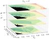 |
Fig. 8 Mutually inclined grids where Ωb,c = 0, and the mutual inclination comes only from Δib,c = ib − ic. The low-eccentricity stable island increases its size by assuming higher mutual inclinations, eventually creating an overlap with the 1σ confidence level from the grid’s best fit (dark green contours). |
We have shown in Sects. 4.2 and 4.3 that we most likely observe the η Cet planetary system nearly edge-on, because we found a maximum of stable fits at sini = 1, in line with the Hipparcos constraint. Assuming lower inclinations, the size of the stability region in the (eb,ec) plane decreases. Because we constrained the system inclination only by stability criteria, it would be interesting to see whether the stability will sufficiently increase if we allow a mutual inclination between the orbits to occur in our fits, or whether the system will become more unstable than for the coplanar fits. Moreover, as we have shown in Sect. 3.2, by adding three additional fitting parameters we obtain significantly better fits (although very unstable), and it is important to determine whether we can find any stable solutions or even stable islands for highly inclined non-coplanar configurations.
To study the dynamics of the η Cet system for mutually inclined orbits we investigated the stability with the following three different strategies:
-
1)
We fixed the Δib,c to be constant and assumed Ωb,c = 0°, so that the mutual inclination depends only on ib,c. We defined Δib,c = ib − ic, where for the 2:1 MMR region the ib = 89.5°, 89°, 88.5° and ic = 90.5°, 91°, 91.5°. We found that the size of the 2:1 MMR stable region decreases very fast with mutual inclination, and after Δib,c> 2° the 2:1 MMR island completely vanishes. For the global (eb,ec) grid we defined ib = 85°, 80°, 75° and ic = 95°, 100°, 105°. The results from this test are illustrated in Fig. 8. From the grid we found that the low-eccentricity stable region shows a trend of expanding its size with the mutual inclination for Δib,c = 10° and 20°. When Δib,c = 30° the stable area expands and we find many stable fits for moderate ec within the 1σ confidence region from the Δib,c = 30° grid. This test shows that for a high mutual inclination there is a high probability for the system to have near circular orbits, or moderate ec.
-
2)
We again relied on the (eb,ec) grids, where additional free parameters in the fits are ib,c and Ωb,c. However, in the fitting we restricted the minimum inclination to be ib,c = 90°, and the sinimax factor comes only from inclination angles above this limit. In this test we only studied the global (eb,ec) plane, without examining the 2:1 MMR region separately. Initially, for the first grid we set sinimax = 0.707 (imax = 135°), while Ωb,c was unconstrained and was let to vary across the full range from 0 to 2π. Later we constructed grids by decreasing the maximum allowed inclination to sinimax = 0.819, 0.906, 0.966 and at last 0.996 (imax = 125°, 115°, 105°, and 95°, respectively), thereby decreasing the upper limit on the planetary masses and mutual inclination angle Δib,c. In all grids we allowed ib ≠ ic, and Ωb ≠ Ωc as we discussed in Sect. 3.2. We find that when increasing imax, the grid’s
values improved, and the planetary
ib,c are
usually close to imax. The obtained ΔΩb,c is
also very low, favoring low mutual inclinations in this test. When imax = 95°
the average mutual inclination over the grid is 0.22°, making the grid nearly coplanar. In
this case the planetary masses are only ~0.5% higher than their minimum, which has a negligible
effect on the stability. However, the very small orbital misalignment in those
systems seems to have a positive influence on the system stability, and we find
slightly more stable fits than for the edge-on coplanar case discussed in Sect.
4.2 (see Fig. 9). At larger imax the
distribution in general has lower
values, but the size of the stability region is decreasing. This is probably due to
the increased planetary masses and the stronger gravitational perturbations in the
dynamical simulations. There is not even one stable solution at imax =
135°, but we have to note that there are many chaotic fits that
survived the 105 yr test, which are not shown in Fig. 9. 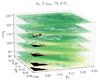
Fig. 9 Grids with mutual inclination dependent on ΔΩb,c and ib,c ≤ imax. During the fitting the mutual inclinations from the grids are very low, on the order of ~ 3°. The stability area has a maximum at imax = 95°, slightly higher than the coplanar grid at 90°. The stability decreases at larger imax due to the larger planetary masses and the stronger perturbations. There is no stable solution at imax = 135°.
-
3)
Because of the resulting low mutual inclination in the second test, we decided to decouple the planetary orbits and to test for higher mutual inclinations by allowing ΔΩb,c ≠ 0, in contrast to the first test where ΔΩb,c = 0. We constructed a grid of best fits for fixed ib,c (ib,ic grid). The planetary inclination ib,c was increased from 90° to 140° with steps of 1°, while rest of the orbital parameters were free in the fitting. This test attempts to check for stability for almost all the possible mutual inclinations in the system. Figure 10 illustrates the stability output in the (ib,ic) plane. The
solutions in this grid have lower
values when ib ≈
ic (close to the
coplanar configuration), and have a clear trend of better fits when the LOS
inclination is high. However, we could not find any stable configuration near the
coplanar diagonal of best fits from ib,c = 90° to
140°. There are many
chaotic survivals and few stable islands at higher mutual inclinations, more than
3σ
away from the grid minimum.
We are aware of the fact that, when including the ib,c and Ωb,c in the fitting model, the parameter space becomes extremely large, and perhaps many more smaller and possibly stable minima might exist, but we have not been able to identify any in this study.
4.5. Impact of stellar mass on the stability analysis
Finally, we have tested how changing the assumed stellar mass influences the stability in
(eb,ec)
space. We generated coplanar edge-on grids by assuming different stellar
masses, using the values in Table 1. We took the
same (eb,ec)
grid area and resolution as discussed in Sect. 4.2
(Fig. 5) and started our grid search with 1
M⊙ and 1.4 M⊙, which are
the lower and upper stellar mass limits for η Cet proposed by Berio et al. (2011). Next we assumed 1.3 M⊙ from Luck & Challener (1995), then 1.84 M⊙, which is the
upper limit from Reffert et al. (2014), and we
already have the 1.7 M⊙ grid from Sect. 4.2. The longest integration time applied to the stability test for
these grids was 105
years.
Stability results are shown in Fig. 11, which clearly shows a trend of higher stability with larger stellar mass. Our starting mass of 1 M⊙ leads almost to the disappearance of the low-eccentricity stable island, and only a few stable solutions can be seen for very circular orbits. Increasing the stellar mass to 1.3 M⊙, 1.4 M⊙ and 1.7 M⊙ reveals larger stable areas at low eccentricities. Finally, in the 1.84 M⊙ grid we see the largest low-eccentricity stable island in our test.
Similarly, the 2:1 MMR region evolves and decreases in size with decreasing η Cet mass. No resonant island is seen at 1 M⊙. However, the 2:1 MMR region has a larger area at 1.7 M⊙ than in the 1.84 M⊙ grid.
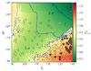 |
Fig. 10 Except for the inclinations, the remaining orbital parameters are free to vary for
the (ib,ic)
grid (50 × 50 fits). The
|
This effect comes from the fact that starting the fitting process with lower stellar mass will also scale down the whole planetary system. The derived orbital angles and the periods from the dynamical fitting will remain almost the same in the (eb,ec) grids when fitting from 1 M⊙ to 1.84 M⊙. However, as can be seen from Eqs. (1), (3) and (4), the planetary masses, semi-major axes ab,c, and the Hill radii rb,c are dependent on the stellar mass. By scaling down the planetary masses, we would expect the gravitational interactions between the planets to be less destructive, and we would thus expect more stable fits when adopting a lower mass for the primary. This is exactly the opposite of what can be seen in Fig. 11. The dynamical simulations are much more sensitive to Δab,c = ac − ab than to the planetary mass ratio. From Eqs. (4) and (5) it can be seen that rb,c will slightly decrease when assuming a lower stellar mass, although not as fast as ab,c will decrease. Δab,c for the 1 M⊙ grid is on average ≈0.54 AU, and for the 1.84 M⊙ grid ≈0.65 AU. The more similar planetary semi-major axes in lower stellar mass systems lead to a higher number of close encounters during the orbital evolution, and thus, to a higher ejection rate, especially for fits with higher eb,c. On the other hand, the Δab,c for the grid with maximum mass for η Cet (1.84 M⊙) is enough to keep the two planets well separated, and the stability region in lower eccentricities increases.
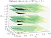 |
Fig. 11 Stability maps with different initial masses for η Cet. A clear stability trend can be seen in the (eb,ec) grids in the sense that by increasing the stellar mass up to the maximum of 1.84 M⊙, the size of the stable region increases as well. |
5. Discussion
5.1. Planetary hypothesis
In principle, the possible reasons for observed RV variability in K giants are rotational modulation of star spots, long-period nonradial pulsations, or the presence of planets.
Star spots can most likely be excluded as a viable explanation for the observed RV
variability of η Cet, at least for one of the two observed periods.
If star spots were to cause the RV to vary, one of the two periods that we observe would
have to match the rotational period (still leaving the second period unexplained).
However, the longest rotation period of η Cet compatible with its radius of R = 14.3 ± 0.2
R⊙ and its projected rotational velocity
vsini = 3.8
± 0.6 km s-1 (Hekker & Meléndez
2007) is 190 days. This is much shorter than either the
405-day or the 750-day period. Moreover, one would expect a larger photometric variation
than the 3 mmag observed by Hipparcos for a star spot to generate an RV amplitude
on the order of 50 m s-1 (Hatzes & Cochran
2000)3. On the other hand, macro-turbulent
surface structures on K giants are currently poorly understood. Large and stable
convection cells could act as velocity spots, yielding an RV variability without
significant photometric variability (e.g., Hatzes &
Cochran 2000). Although unlikely, we cannot fully exclude that the shorter
405-day period is due to rotational modulation of surface features, while the longer
750-day period is most certainly due to a planet.
days. This is much shorter than either the
405-day or the 750-day period. Moreover, one would expect a larger photometric variation
than the 3 mmag observed by Hipparcos for a star spot to generate an RV amplitude
on the order of 50 m s-1 (Hatzes & Cochran
2000)3. On the other hand, macro-turbulent
surface structures on K giants are currently poorly understood. Large and stable
convection cells could act as velocity spots, yielding an RV variability without
significant photometric variability (e.g., Hatzes &
Cochran 2000). Although unlikely, we cannot fully exclude that the shorter
405-day period is due to rotational modulation of surface features, while the longer
750-day period is most certainly due to a planet.
Ruling out nonradial pulsations is harder than ruling out star spots, but also possible.
First, we see evidence of eccentricity in the shape of the radial velocity curves, which
is an indication for a Keplerian orbit. Second, the signal has been consistent over 12
years; this is not necessarily expected for pulsations. Third, on top of the optical RV
data we derived the RV from the infrared wavelength regime (CRIRES). Although the IR RV
error is much larger than that from the optical data, the CRIRES data are clearly
consistent with the Lick data. The best dynamical fit derived from the
visible data and applied only to the near-IR data has
 and rms = 26.7 m s-1, while a constant model
assuming no planets has
and rms = 26.7 m s-1, while a constant model
assuming no planets has  and rms = 63.2 m s-1. Therefore, the two-planet fit
is more likely. Just based on the CRIRES data, we can rule out infrared amplitudes smaller
than 30 m s-1 or
larger than 65 m s-1 with 68.3% confidence. If the RV variability in the
optical were to be caused by pulsations, one might expected to find a different amplitude
in the IR, which is not the case. Fourth, there are no indications for these long-period
nonradial pulsations in K giants yet, although a variety of very short pulsation modes
have been found with Kepler (Bedding
et al. 2011). Taken together, there is no supporting evidence for the presence of
pulsations in η Cet.
and rms = 63.2 m s-1. Therefore, the two-planet fit
is more likely. Just based on the CRIRES data, we can rule out infrared amplitudes smaller
than 30 m s-1 or
larger than 65 m s-1 with 68.3% confidence. If the RV variability in the
optical were to be caused by pulsations, one might expected to find a different amplitude
in the IR, which is not the case. Fourth, there are no indications for these long-period
nonradial pulsations in K giants yet, although a variety of very short pulsation modes
have been found with Kepler (Bedding
et al. 2011). Taken together, there is no supporting evidence for the presence of
pulsations in η Cet.
The strongest evidence supporting a multiple planetary system comes from the dynamical modeling of the RV data. Taking the gravitational interactions between the two planets into account leads to a considerably better fit than the two Keplerian model (or two sinusoids). In other words, we were able to detect the interactions between the two planets in our data, which strongly supports the existence of the two planets.
Thus, though we cannot completely rule out alternative explanations, a two-planet system is the most plausible interpretation for the observed RV variations of η Cet.
5.2. Giant star planetary population
With the detection of the first extrasolar planet around the giant star ι Dra b (the first planet announced from our Lick sample – Frink et al. 2002) the search for planets around evolved intermediate mass stars has increased very rapidly. Several extrasolar planet search groups are working in this field to provide important statistics for planet occurrence rates as a function of stellar mass, evolutionary status, and metallicity (Frink et al. 2001; Sato et al. 2003; Hatzes et al. 2006; Niedzielski et al. 2007; Döllinger et al. 2009; Mitchell et al. 2013,etc.). Up to date, there are 56 known planets around 53 giants stars in the literature, and all of them are in wide orbits.
Except for the η Cet discovery, there are only three candidate multiple planetary systems known to orbit giant stars, and all of them show evidence of two massive substellar companions. Niedzielski et al. (2009a,b) reported planetary systems around the K giants HD 102272 and BD +20 2457. While the published radial velocity measurements of HD 102272 are best modeled with a double Keplerian, the sparse data sampling is insufficient to derive an acurate orbit for the second planet. Initial stability tests based on the published orbital parameters show a very fast collision between the planets. This appears to be due to the presumably very eccentric orbit of the outer planet, which leads to close encounters, making the system unstable. The case of BD +20 2457 is even more dramatic. The best-fit solution suggests a brown dwarf and a very massive planet just at the brown dwarf mass border, with minimum masses of m1sini1 ≈ 21.4 MJup and m2sini2 ≈ 12.5 MJup, respectively (1 is the inner and 2 the outer planet). This system has very similar orbital periods of P1 ≈ 380 days and P2 ≈ 622 days for such a massive pair, and the gravitational interactions are extremely destructive. We have tested several orbital parameter sets within the derived parameter errors and, without conducting any comprehensive stability analysis, so far we were unable to find any stable configuration for BD +20 2457. Recently, Horner et al. (2014) investigated the stability of BD +20 2457 in more detail and did not find any stable solutions either. However, we have to keep in mind that the formal best fit for η Cet was also unstable, and only after an extensive stability analysis did we find long-term stable regions. In this context we do not exclude the possibility that HD 102272 and BD +20 2457 indeed harbor multiple planetary systems, but better data sampling is required to better constrain the planetary orbits. Moreover, additional efforts must be undertaken to prove the stability for these two systems, perhaps including highly mutually inclined configurations, or even better constraints on the stellar masses.
Of particular interest is also the system around the K giant ν Oph (Quirrenbach et al. 2011; Sato et al. 2012), which is consistent with two brown dwarfs with masses m1sini1 ≈ 22.3 MJup, m2sini2 ≈ 24.5 MJup. The two brown dwarfs exhibit a clear 6:1 MMR, with periods of P1 ≈ 530 days and P2 ≈ 3190 days.
Although ν Oph and potentially BD +20 2457 are not planetary systems, they may present important evidence for brown dwarf formation in a circumstellar disk. Such objects may form because in general the more massive stars should have more massive disks from which protoplanetary objects can gain enough mass to become brown dwarfs. It might be possible for the 6:1 resonance configuration of ν Oph to have formed via migration capture in a protoplanetary disk around a young intermediate-mass progenitor, and the brown dwarf occurrence may be rather high (Quirrenbach et al. 2011).
Therefore, if we exclude ν Oph, which is clearly a brown dwarf system, and the HD 102272 and BD +20 2457 systems, which suffer from poor data sampling and stability problems, η Cet is currently the only K giant star that shows strong evidence for harboring a stable multiplanetary system.
5.3. Unique orbital configuration of η Cet
The stable solutions from the 2:1 MMR region in the edge-on coplanar and inclined tests raise some important questions about the possible formation and evolution of the η Cet planetary system. The θb ≈ 0° and θc ≈ 180° 2:1 MMR configuration is similar to that of the 2:1 resonance between the Jovian satellites Io and Europa, but the Io-Europa configuration is not supposed to exist for relatively large eccentricities (see Beaugé et al. 2003; Lee 2004). The average eb (~0.2) and ec (~0.05) for η Cet are much larger than the eb,ec boundary where the θb ≈ 0° and θc ≈ 180° configuration exists. An aligned configuration with both θb and θc librating about 0° is expected for a mass ratio mb/mc ≈ 0.77 and the eccentricities in the 2:1 MMR region.
One possible stabilizing mechanism for the η Cet system might be the large libration amplitudes of both θb and θc, which are almost circulating. We made some preliminary attempts and failed to find a small libration amplitude counterpart. More work is needed to understand the stability of this 2:1 MMR configuration, as well as its origin, if η Cet is indeed in this configuration.
We cannot fully exclude that the true system configuration of η Cet corresponds to some of the single isolated stable fits that we see in the stability maps, and neither can we exclude one of the numerous fits that are stable for 108 years, which show a scattering chaotic behavior. A nonresonant system in near circular orbits is also possible.
6. Summary
We have reported the discovery of a planetary system around the K giant star η Cet. This discovery is the result of a long-term survey, which aims to discover planetary companions around 373 intermediate-mass G and K giant stars, and which started back in 1999 at Lick Observatory. We presented 118 high-precision optical radial velocities based on the observations with the Hamilton spectrograph at Lick Observatory and nine near-infrared data points from the ESO CRIRES spectrograph; these data cover more than a decade.
We have fitted a dynamical model to the optical data, which ensured that any possible
gravitational interactions between the planets are taken into account in the fitting
process. We showed that the dynamical model represents a significant
improvement over the double-Keplerian fit.
In an attempt to characterize the most likely planetary configuration, we performed an
extensive stability analysis of the η Cet system. We made a wide variety of
high-resolution co-planar and inclined dynamical grids, which we used as an input for our
numerical analysis. Thus, we transformed these grids into detailed stability maps. In total,
we carried out more than 200 000 dynamical integrations with typical time spans of
105 and
2 × 10⁶ years, and
we extended the test to 108 years to study the edge-on coplanar case.
For the edge-on coplanar grid we used a set of best fits for fixed eb and ec. We found that the η Cet system can be stable for at least 108 years, locked in a 2:1 MMR in a region with moderate eb, which lies about 1σ away from the best co-planar fit. A much larger nonresonant stable region exists with nearly circular orbits, although it is located more than 3σ away from the best fit and is thus less likely. In the 2:1 MMR region all fits are in an anti-aligned planetary configuration and very close to the separatrix. The low-order eccentricity-type resonant angles θb and θc librate around 0° and 180°, respectively, but with very large amplitudes of ≈±180°. A similar near-separatrix behavior can be seen in the stable fits with near circular orbits, where the secular resonance angle Δωb,c circulates, but during most of the simulation the planetary configuration is anti-aligned (Δωb,c ≈ 180°).
We provided a detailed set of (eb,ec) coplanar inclined stability maps, showing that the η Cet system is very likely observed in a near edge-on configuration (ib,c ≈ 90°). The size of the stable region is largest when the system is assumed to have ib,c = 90°, and when we increased the planetary mass via sinib,c, the size of the two stability regions in the (eb, ec) plane decreased. The 2:1 MMR stable island totally disappeared when ib,c ≈ 70°, while the near circular stable island survived until the LOS inclination becomes ib,c ~ 49°. Below the last inclination limit, all the fits in the (eb, ec) plane became unstable.
We also presented results from a grid based on mutually inclined configurations, although we pointed out that they need not be exhaustive. This is because of the large amount of computational time needed when the parameter space is expanded. Another way of constraining the mutual inclination would be a very extensive and precise radial velocity and astrometric data set, which is so far not available for η Cet.
The most important conclusion from the inclined dynamical test is that the planets cannot be more massive than a factor of ~1.4 heavier than their suggested minimum masses. Higher inclinations, and thus larger planetary masses, lead to instability in all cases. This excludes the possibility of two brown dwarfs purely based on stability considerations, and strongly favors a planetary system.
We also tested how the uncertainty of the stellar mass will affect the dynamical stability of the system. Decreasing the stellar mass leads to a smaller size of the stable region in the (eb,ec) grids, and thus we conclude that the stellar mass value from Reffert et al. (2014) is indeed a very reasonable estimate.
The η Cet system is only the fourth candidate multiple substellar system around a G or K giant star and presents an important milestone for understanding planetary formation and evolution as a function of stellar mass, metallicity, and age.
The Hipparcos observations were taken earlier (until 1993) than our RV data (since 2000), but assuming that η Cet was quiet for four years, and active with a very constant RV amplitude for more than ten years just seven years later appears rather contrived.
Acknowledgments
Part of this work was supported by the International Max Planck Research School for Astronomy and Cosmic Physics at the University of Heidelberg, IMPRS-HD, Germany. M.H.L. was supported in part by the Hong Kong RGC grant HKU 7024/13P. We would like to thank the staff at Lick Observatory for their support over the years of this project. We kindly thank the CAT observers that assisted with this project, including Saskia Hekker, Simon Albrecht, David Bauer, Christoph Bergmann, Stanley Browne, Kelsey Clubb, Dennis Kügler, Christian Schwab, Julian Stürmer, Kirsten Vincke, and Dominika Wylezalek. We thank Mathias Zechmeister and Ansgar Reiners for their help with the acquisition and reduction of the CRIRES data. We thank Stefano Meschiari for the very helpful discussion regarding the capabilities of the Console package. We would also like to thank our referee, Artie Hatzes, for his constructive comments that helped to improve this paper.
References
- Baranne, A., Queloz, D., Mayor, M., et al. 1996, A&AS, 119, 373 [NASA ADS] [CrossRef] [EDP Sciences] [Google Scholar]
- Barban, C., De Ridder, J., Mazumdar, A., et al. 2004, in SOHO 14 Helio- and Asteroseismology: Towards a Golden Future, ed. D. Danesy, ESA SP, 559, 113 [Google Scholar]
- Bean, J. L., & Seifahrt, A. 2009, A&A, 496, 249 [NASA ADS] [CrossRef] [EDP Sciences] [MathSciNet] [Google Scholar]
- Bean, J. L., Seifahrt, A., Hartman, H., et al. 2010, ApJ, 711, L19 [NASA ADS] [CrossRef] [Google Scholar]
- Beaugé, C., Ferraz-Mello, S., & Michtchenko, T. A. 2003, ApJ, 593, 1124 [Google Scholar]
- Bedding, T. R., Mosser, B., Huber, D., et al. 2011, Nature, 471, 608 [NASA ADS] [CrossRef] [PubMed] [Google Scholar]
- Berio, P., Merle, T., Thévenin, F., et al. 2011, A&A, 535, A59 [NASA ADS] [CrossRef] [EDP Sciences] [Google Scholar]
- Butler, R. P., Marcy, G. W., Williams, E., et al. 1996, PASP, 108, 500 [NASA ADS] [CrossRef] [Google Scholar]
- Butler, R. P., Marcy, G. W., Williams, E., Hauser, H., & Shirts, P. 1997, ApJ, 474, L115 [NASA ADS] [CrossRef] [Google Scholar]
- Butler, R. P., Marcy, G. W., Fischer, D. A., et al. 1999, ApJ, 526, 916 [NASA ADS] [CrossRef] [Google Scholar]
- Chambers, J. E. 1999, MNRAS, 304, 793 [NASA ADS] [CrossRef] [MathSciNet] [Google Scholar]
- Correia, A. C. M., Udry, S., Mayor, M., et al. 2009, A&A, 496, 521 [NASA ADS] [CrossRef] [EDP Sciences] [Google Scholar]
- De Ridder, J., Barban, C., Carrier, F., et al. 2006, A&A, 448, 689 [NASA ADS] [CrossRef] [EDP Sciences] [Google Scholar]
- Desort, M., Lagrange, A.-M., Galland, F., et al. 2008, A&A, 491, 883 [NASA ADS] [CrossRef] [EDP Sciences] [Google Scholar]
- Döllinger, M. P., Hatzes, A. P., Pasquini, L., et al. 2009, A&A, 499, 935 [NASA ADS] [CrossRef] [EDP Sciences] [Google Scholar]
- Duncan, M. J., Levison, H. F., & Lee, M. H. 1998, AJ, 116, 2067 [NASA ADS] [CrossRef] [EDP Sciences] [Google Scholar]
- Figueira, P., Pepe, F., Melo, C. H. F., et al. 2010, A&A, 511, A55 [NASA ADS] [CrossRef] [EDP Sciences] [Google Scholar]
- Fischer, D. A., Marcy, G. W., Butler, R. P., Laughlin, G., & Vogt, S. S. 2002, ApJ, 564, 1028 [NASA ADS] [CrossRef] [Google Scholar]
- Fischer, D. A., Marcy, G. W., Butler, R. P., et al. 2003, ApJ, 586, 1394 [NASA ADS] [CrossRef] [Google Scholar]
- Fischer, D. A., Marcy, G. W., Butler, R. P., et al. 2008, ApJ, 675, 790 [NASA ADS] [CrossRef] [Google Scholar]
- Ford, E. B. 2005, AJ, 129, 1706 [Google Scholar]
- Frandsen, S., Carrier, F., Aerts, C., et al. 2002, A&A, 394, L5 [NASA ADS] [CrossRef] [EDP Sciences] [Google Scholar]
- Frink, S., Quirrenbach, A., Fischer, D., Röser, S., & Schilbach, E. 2001, PASP, 113, 173 [NASA ADS] [CrossRef] [Google Scholar]
- Frink, S., Mitchell, D. S., Quirrenbach, A., et al. 2002, ApJ, 576, 478 [NASA ADS] [CrossRef] [MathSciNet] [Google Scholar]
- Gaudi, B. S., Bennett, D. P., Udalski, A., et al. 2008, Science, 319, 927 [NASA ADS] [CrossRef] [PubMed] [Google Scholar]
- Girardi, L., Bressan, A., Bertelli, G., & Chiosi, C. 2000, A&AS, 141, 371 [NASA ADS] [CrossRef] [EDP Sciences] [Google Scholar]
- Gray, R. O., Corbally, C. J., Garrison, R. F., et al. 2006, AJ, 132, 161 [NASA ADS] [CrossRef] [Google Scholar]
- Hamilton, D. P., & Burns, J. A. 1992, Icarus, 96, 43 [NASA ADS] [CrossRef] [Google Scholar]
- Hatzes, A. P., & Cochran, W. D. 2000, AJ, 120, 979 [NASA ADS] [CrossRef] [Google Scholar]
- Hatzes, A. P., Cochran, W. D., Endl, M., et al. 2006, A&A, 457, 335 [NASA ADS] [CrossRef] [EDP Sciences] [Google Scholar]
- Hekker, S., & Meléndez, J. 2007, A&A, 475, 1003 [NASA ADS] [CrossRef] [EDP Sciences] [Google Scholar]
- Hinkle, K., Wallace, L., & Livingston, W. 1995, PASP, 107, 1042 [NASA ADS] [CrossRef] [Google Scholar]
- Horner, J., Wittenmyer, R. A., Hinse, T. C., & Marshall, J. P. 2014, MNRAS, 439, 1176 [NASA ADS] [CrossRef] [Google Scholar]
- Huélamo, N., Figueira, P., Bonfils, X., et al. 2008, A&A, 489, L9 [NASA ADS] [CrossRef] [EDP Sciences] [Google Scholar]
- Kaeufl, H.-U., Ballester, P., Biereichel, P., et al. 2004, in Proc. SPIE 5492, eds. A. F. M. Moorwood, & M. Iye, 1218 [Google Scholar]
- Kjeldsen, H., & Bedding, T. R. 1995, A&A, 293, 87 [NASA ADS] [Google Scholar]
- Kjeldsen, H., & Bedding, T. R. 2011, A&A, 529, A8 [NASA ADS] [CrossRef] [EDP Sciences] [Google Scholar]
- Kupka, F., Piskunov, N., Ryabchikova, T. A., Stempels, H. C., & Weiss, W. W. 1999, A&AS, 138, 119 [NASA ADS] [CrossRef] [EDP Sciences] [MathSciNet] [PubMed] [Google Scholar]
- Laskar, J., & Correia, A. C. M. 2009, A&A, 496, L5 [NASA ADS] [CrossRef] [EDP Sciences] [Google Scholar]
- Laughlin, G., Chambers, J., & Fischer, D. 2002, ApJ, 579, 455 [NASA ADS] [CrossRef] [Google Scholar]
- Lee, J. W., Kim, S.-L., Kim, C.-H., et al. 2009, AJ, 137, 3181 [NASA ADS] [CrossRef] [Google Scholar]
- Lee, M. H. 2004, ApJ, 611, 517 [NASA ADS] [CrossRef] [Google Scholar]
- Lee, M. H., & Peale, S. J. 2002, ApJ, 567, 596 [NASA ADS] [CrossRef] [Google Scholar]
- Lee, M. H., & Peale, S. J. 2003, ApJ, 592, 1201 [NASA ADS] [CrossRef] [Google Scholar]
- Lovis, C., Ségransan, D., Mayor, M., et al. 2011, A&A, 528, A112 [NASA ADS] [CrossRef] [EDP Sciences] [Google Scholar]
- Luck, R. E., & Challener, S. L. 1995, AJ, 110, 2968 [NASA ADS] [CrossRef] [Google Scholar]
- Marcy, G. W., & Butler, R. P. 1992, PASP, 104, 270 [NASA ADS] [CrossRef] [Google Scholar]
- Marcy, G. W., Butler, R. P., Fischer, D., et al. 2001, ApJ, 556, 296 [NASA ADS] [CrossRef] [Google Scholar]
- Marois, C., Zuckerman, B., Konopacky, Q. M., Macintosh, B., & Barman, T. 2010, Nature, 468, 1080 [NASA ADS] [CrossRef] [PubMed] [Google Scholar]
- Mayor, M., & Queloz, D. 1995, Nature, 378, 355 [NASA ADS] [CrossRef] [Google Scholar]
- Meschiari, S., Wolf, A. S., Rivera, E., et al. 2009, PASP, 121, 1016 [NASA ADS] [CrossRef] [Google Scholar]
- Mitchell, D. S., Reffert, S., Trifonov, T., Quirrenbach, A., & Fischer, D. A. 2013, A&A, 555, A87 [NASA ADS] [CrossRef] [EDP Sciences] [Google Scholar]
- Niedzielski, A., Konacki, M., Wolszczan, A., et al. 2007, ApJ, 669, 1354 [NASA ADS] [CrossRef] [Google Scholar]
- Niedzielski, A., Goździewski, K., Wolszczan, A., et al. 2009a, ApJ, 693, 276 [NASA ADS] [CrossRef] [Google Scholar]
- Niedzielski, A., Nowak, G., Adamów, M., & Wolszczan, A. 2009b, ApJ, 707, 768 [NASA ADS] [CrossRef] [Google Scholar]
- Percy, J. R., Wilson, J. B., & Henry, G. W. 2001, PASP, 113, 983 [NASA ADS] [CrossRef] [Google Scholar]
- Press, W. H., Teukolsky, S. A., Vetterling, W. T., & Flannery, B. P. 1992, Numerical Recipes in FORTRAN, The art of scientific computing, 2nd edn (Cambridge University Press) [Google Scholar]
- Prugniel, P., Vauglin, I., & Koleva, M. 2011, A&A, 531, A165 [NASA ADS] [CrossRef] [EDP Sciences] [Google Scholar]
- Quirrenbach, A., Reffert, S., & Bergmann, C. 2011, in AIP Conf. Proc., 1331, eds. S. Schuh, H. Drechsel, & U. Heber, 102 [Google Scholar]
- Reffert, S., & Quirrenbach, A. 2011, A&A, 527, A140 [NASA ADS] [CrossRef] [EDP Sciences] [Google Scholar]
- Reffert, S., Christoph Bergmann, C., Quirrenbach, A., et al. 2014, A&A, submitted [Google Scholar]
- Rivera, E. J., Laughlin, G., Butler, R. P., et al. 2010, ApJ, 719, 890 [Google Scholar]
- Rothman, L. S., Rinsland, C. P., Goldman, A., et al. 1998, J. Quant. Spec. Radiat. Transf., 60, 665 [NASA ADS] [CrossRef] [Google Scholar]
- Sato, B., Ando, H., Kambe, E., et al. 2003, ApJ, 597, L157 [NASA ADS] [CrossRef] [Google Scholar]
- Sato, B., Omiya, M., Harakawa, H., et al. 2012, PASJ, 64, 135 [NASA ADS] [CrossRef] [Google Scholar]
- Seifahrt, A., & Käufl, H. U. 2008, A&A, 491, 929 [NASA ADS] [CrossRef] [EDP Sciences] [Google Scholar]
- Tan, X., Payne, M. J., Lee, M. H., et al. 2013, ApJ, 777, 101 [NASA ADS] [CrossRef] [Google Scholar]
- Tuomi, M. 2012, A&A, 543, A52 [NASA ADS] [CrossRef] [EDP Sciences] [Google Scholar]
- Valenti, J. A., Butler, R. P., & Marcy, G. W. 1995, PASP, 107, 966 [NASA ADS] [CrossRef] [Google Scholar]
- van Leeuwen, F. 2007, A&A, 474, 653 [NASA ADS] [CrossRef] [EDP Sciences] [Google Scholar]
- Wolszczan, A., & Frail, D. A. 1992, Nature, 355, 145 [NASA ADS] [CrossRef] [Google Scholar]
- Zechmeister, M., Reffert, S., Hatzes, A. P., Endl, M., & Quirrenbach, A. 2008, A&A, 491, 531 [NASA ADS] [CrossRef] [EDP Sciences] [Google Scholar]
All Tables
All Figures
|
Fig. 1 Top panel: radial velocities measured at Lick Observatory (blue circles), along with error bars, covering about 11 years from July 2000 to October 2011. Two best fits to the Lick data are overplotted: a double-Keplerian fit (dot-dashed) and the best dynamical edge-on coplanar fit (solid line). The two fits are not consistent in later epochs because of the gravitational interactions considered in the dynamical model. Despite the large estimated errors, the data from CRIRES (red diamonds) seem to follow the best fit prediction from the dynamical fit. Bottom panel: no systematics are visible in the residuals. The remaining radial velocity scatter has a standard deviation of 15.9 m s-1, most likely caused by rapid solar – like p – mode oscillations. |
| In the text | |
|
Fig. 2 Top panel: the periodogram of the measured radial velocities shows two highly significant peaks around 399 and 768 days, while the Kepler fit to the data reveals a best fit at periods around 403.5 and 751.9 days. Bottom panel: no significant peak is left in the periodogram of the residuals after removing the two periods from the Keplerian fit. |
| In the text | |
|
Fig. 3 Intrinsic RV scatter observed in our sample of 373 K giants versus B – V color. A clear trend is visible in the sense that redder stars without companions (circles) have larger intrinsic RV variations. A number of stars lie above the almost linear relation between color and the logarithm of the scatter. These stars have clearly periodic RVs, which indicates that they harbor substellar or stellar companions. Stars with non-periodic, but still systematic radial velocities are indicated with green crosses. The RV scatter of ~15 m s-1, for η Cet (red star) derived as the rms around the orbital fit, is lower than the 25 m s-1 derived from the linear trend at the star’s color index. |
| In the text | |
|
Fig. 4 Semi-major axes evolution of the best dynamical fits. Left: the edge-on coplanar fit remains stable in a 2:1 MMR only for 17 000 years, when the system starts to show chaotic behavior and eventually ejects the outer planet. The best inclined coplanar (middle) and mutually inclined (right) fits fail to preserve stability even on very short timescales. |
| In the text | |
|
Fig. 5 Right: edge-on coplanar |
| In the text | |
|
Fig. 6 Evolution of the orbital parameters for three different fits, stable for at least 108 years. The best 2:1 MMR fit (left panels), the best stable fit from the low-eccentricity region (middle panels), and the fit with the most circular orbits (right panels). In the 2:1 MMR fit the gravitational perturbation between the planets is much larger than in the other two cases. It is easy to see that eccentricities for given epochs can be much larger than their values at the initial epoch of the integration. For convenience the evolution of the semi-major axes, eccentricities, the resonant angles (third row) and the Δωb,c are given for 500 and 105 years, respectively. The bottom row gives the orbital precession region, the sum of orbits for each integration output. |
| In the text | |
|
Fig. 7 Coplanar inclined grids illustrate the stability dependence on mb,csinib,c. Color maps are the same as in Fig. 5, with the difference that for clarity, only the stable regions are shown (black). The top layer shows the grids from Fig. 5, where sinib,c = 1 (ib,c = 90°). Decreasing the inclination leads to smaller near-circular and 2:1 MMR stability regions. The resonant region shrinks and moves in the (eb,ec) plane, and it completely vanishes when sini ≤ 0.93. The stable island at low eccentricities vanishes for sini ≤ 0.75, when even the most circular (eb,c = 0.001) fit is unstable. |
| In the text | |
|
Fig. 8 Mutually inclined grids where Ωb,c = 0, and the mutual inclination comes only from Δib,c = ib − ic. The low-eccentricity stable island increases its size by assuming higher mutual inclinations, eventually creating an overlap with the 1σ confidence level from the grid’s best fit (dark green contours). |
| In the text | |
|
Fig. 9 Grids with mutual inclination dependent on ΔΩb,c and ib,c ≤ imax. During the fitting the mutual inclinations from the grids are very low, on the order of ~ 3°. The stability area has a maximum at imax = 95°, slightly higher than the coplanar grid at 90°. The stability decreases at larger imax due to the larger planetary masses and the stronger perturbations. There is no stable solution at imax = 135°. |
| In the text | |
|
Fig. 10 Except for the inclinations, the remaining orbital parameters are free to vary for
the (ib,ic)
grid (50 × 50 fits). The
|
| In the text | |
|
Fig. 11 Stability maps with different initial masses for η Cet. A clear stability trend can be seen in the (eb,ec) grids in the sense that by increasing the stellar mass up to the maximum of 1.84 M⊙, the size of the stable region increases as well. |
| In the text | |
Current usage metrics show cumulative count of Article Views (full-text article views including HTML views, PDF and ePub downloads, according to the available data) and Abstracts Views on Vision4Press platform.
Data correspond to usage on the plateform after 2015. The current usage metrics is available 48-96 hours after online publication and is updated daily on week days.
Initial download of the metrics may take a while.