| Issue |
A&A
Volume 568, August 2014
|
|
|---|---|---|
| Article Number | A52 | |
| Number of page(s) | 14 | |
| Section | Cosmology (including clusters of galaxies) | |
| DOI | https://doi.org/10.1051/0004-6361/201322355 | |
| Published online | 13 August 2014 | |
Local reionization histories with a merger tree of the HII regions
1
Kavli Institute for Cosmology and Institute of Astronomy,
Madingley Rd,
Cambridge
CB3 0HA,
UK
e-mail:
This email address is being protected from spambots. You need JavaScript enabled to view it.
2
Université de Strasbourg, CNRS UMR 7550, 11 rue de l’Université, 67000
Strasbourg,
France
Received:
24
July
2013
Accepted:
25
June
2014
Abstract
Aims. We investigate simple properties of the initial stage of the reionization process around progenitors of galaxies, such as the extent of the initial HII region before its fusion with the UV background, and the duration of its propagation.
Methods. We used a set of four reionization simulations with different resolutions and ionizing source prescriptions. By using a merger tree of the HII regions we compiled a catalog of the HII region properties. When the ionized regions undergo a major-merger event, we considered that they belong to the global UV background. From the lifetime of the region and from their volume until this moment we drew typical local reionization histories as a function of time and investigated the relation between these histories and the halo mass progenitors of the regions. We then used an average mass accretion history model (AMAH) to extrapolate the halo mass inside the region from high z to z = 0 to predict the past reionization histories of galaxies we see today.
Results. We found that the later an HII region appears during the reionization period, the shorter their related lifetime is and the smaller their volume before they merge with the global UV background. Quantitatively, the duration and extent of the initial growth of an HII region is strongly dependent on the mass of the inner halo and can be as long as ~50% of the reionization epoch. We found that the more massive a halo is today, the earlier it appears and the larger is the extension and the longer the propagation duration of its HII region. Quantitative predictions differ depending on the box size or the source model: small simulated volumes are affected by proximity effects between HII regions, and halo-based source models predict smaller regions and slower I-front expansion than models that use star particles as ionizing sources. Applying this extrapolation to Milky Way-type halos leads to a maximal extent of 1.1 Mpc/h for the initial HII region that established itself in ~150−200 ± 20 Myr. This is consistent with the prediction made using constrained Local Group simulations. For halos with masses similar to those of the Local Group (MW + M31), our result suggests that statistically it has not been influenced by an external front coming from a Virgo-like cluster.
Key words: dark ages, reionization, first stars / galaxies: high-redshift / radiative transfer
© ESO, 2014
1. Introduction
The reionization is a global transition event that saw the neutral atomic content of the Universe changed back to an ionized state. This transition would end between z ~ 11 (Komatsu et al. 2009) and z ~ 6 (Fan et al. 2006; Willott et al. 2007), respectively, according to observations of the diffusion of cosmic microwave background (CMB) photons on the electrons released during reionization and the absorption features in the spectra of high-redshift quasars. It is now a challenge to properly understand this period to explain the impact the radiation of the first sources had, as well as their imprints on the structure formation or the temperature evolution.
But reionization is also a local process, at least in its earliest stages. Before the large ionized patches overlap toward the end of the process, the onset and the growth of HII regions is expected to present a scatter that depends at least partly on local properties. For instance, a typical cosmic reionization history presents a sharp drop in neutral fraction between z = 9 and z = 6, whereas specific regions have obviously been reionized for a few hundred millions of years at this stage: the history of the average neutral fraction is not necessarily representative of any local reionization history. This is especially true around sources hosted by galaxy progenitors that reionized first. The ionisation front (I-front) propagations, the recombination rates, and the merging of small local ionized patches for example depend on the local source and baryon distribution as well as on their local evolution. In a modelization context where reionization may provide an answer for example to the missing satellite problem, it is of prime importance to know whether the rise of the UV flux is similar to an average cosmic background or conversely is strictly constrained by the local buildup of sources and I-fronts. An example are the dwarf galaxies in the Local Group that present well established number and radial distributions that challenge the standard LCDM framework (see Klypin et al. 1999; Moore et al. 1999). It has been suggested that a local reionization process (see, e.g., Ocvirk & Aubert 2011 or Ocvirk et al. 2013), with UV photons produced by a central lighthouse (such as the Milky Way or M31) could provide a radiative feedback that leads to better fits to the data than an external UV background. This suggests that the Local Group experienced a local inside-out reionization, isolated from external contributions for a sufficient time. The question then is whether this assumption is reasonable for the constituents of the Local Group, and whether it is a frequent or a peculiar configuration. More generally, how long does it take for a galaxy to be influenced by the cosmological UV background, and might the duration of its isolation be crucial to the initial buildup of its stellar and baryonic content? Hereafter we name this process local reionization for this initial growth of an HII region in isolation, before it finally connects with the great patches that establish the UV background.
Currently, much effort has been made in order to properly model the phenomena thanks to the advent of cosmological radiative transfer codes (see Iliev et al. 2006a, 2009; and Iliev et al. 2009 for a comparison between these codes). The radiative transfer runs can be realized on dark matter fields by directly considering the dark matter halos as ionizing source sites and the dark matter as a good tracer of the gas (see Iliev et al. 2006b, 2007; Mellema et al. 2006, for example). The runs can also be post-processed on hydrodynamical simulations that previously generate a field of star particles that are assumed to be ionizing sources (see Aubert & Teyssier 2010; and Chardin et al. 2012, among others). Finally, recently, some authors have begun to include the radiative transfer steps directly during the hydrodynamical evolution steps of the gas (see Krumholz et al. 2007; Hasegawa & Umemura 2010; Wise & Abel 2011; Finlator et al. 2011). These new methods enable apprehending the retro-action of the radiation on the star formation and allow us to achieve increasingly realistic simulations of the reionization process.
Previous authors have focused their investigations on the evolution of the HII regions in simulations of cosmic reionization. Studies on static HII region fields taken at different redshifts were made to characterize the HII region sizes (see Furlanetto et al. 2004, 2006; Zahn et al. 2007; Shin et al. 2008) or shape (see McQuinn et al. 2007; and Croft & Altay 2008, for example). Recently, Friedrich et al. (2011) have focused on the evolution of the HII region sizes during entire simulations with the idea of characterizing the impact of the method used for the HII region detection. Recently, Chardin et al. (2012) studied such a dynamical evolution in cosmological simulations by using a merger tree of the HII regions, which is similar to previously employed methodology that was used to investigate the assembly history of dark matter halos in simulations (see, e.g., Roukema et al. 1993; Roukema & Yoshii 1993; Lacey & Cole 1993; Roukema et al. 1997). Such a merger tree aims at tracking the evolution of the properties of each HII region that appeared during a simulation, such as their volume or merger rate. We showed that this methodology was able to constrain the impact of simulation parameters, such as the ionizing source recipes or the resolution, on the global morphology of the process. In essence, this technique focuses on the average behavior of individual reionization histories (⟨ xion(t) ⟩) instead of on the behavior of the average reionization history (⟨ xion ⟩ (t)).
We here propose to show that the merger tree methodology enables us to proceed by characterizing the local reionization histories induced by a single or a few galaxies. Our main ambition is to investigate some simple properties of these initial local stages of reionization such as
-
the isolation duration, that is the time it takes for an HII region tomerge with the large ionized patches that make up the UVbackground, and
-
the final volume, that is the size of these patches when they become part of the overlapping process.
We track their evolution during the reionization epoch (for z> 6) as well as their dependence on the local dark matter halos mass.
For this purpose, we ran cosmological simulations with radiative post-processing to produce realistic reionization histories down to z ~ 6 and compiled evolution catalogs of the HII region properties for each of the ionized patches detected during a given simulation. This catalog allows us to study the ionized-region properties, such as their volume or lifetime, before they merge with the UV background.
We proceed from this to show that this study allows us to link the past local reionization properties with galaxies that we observe today. We use an average mass accretion history (AMAH) model following Wechsler et al. (2002) to calculate the mass M0 that the dark matter halo progenitors of the HII regions would have today at z = 0. Then, we investigate the relation between these masses and the lifetime or the volume of the related ionized regions before they merge with the UV background.
This paper is organized as follows: in Sect. 2, we present the simulation properties. Then, in Sect. 3 we detail the methodology used to investigate the local reionization properties in the simulations. In Sect. 4 we present the results directly extracted from the simulations before predicting the reionization histories of galaxies seen today in Sect. 5. We discuss the validity of our results and offer some predictions about the Local Group reionization history in Sect. 6. We finally conclude and show the prospects that naturally arise from this study in Sect. 7.
2. Simulations
The simulations used in the current analysis were produced for the investigations described in Aubert & Teyssier (2010), and full details can be found in this article. The same set of simulated data has also been used in Chardin et al. (2012), where an extensive discussion of the UV source models is provided. Therefore we limit the description of the simulations to the most important general features.
2.1. Gas dynamics and radiative post-processing
The dynamics of the gas and dark matter is provided by the simulation code RAMSES, which handles the related physics on adaptive meshes that increase resolution where required. Gas dynamics is solved with to a second-order Godunov scheme combined with an HLLC Riemann solver. Collisionless dynamics is tracked from dark matter particles according to a gravitational potential provided by a multiresolution multigrid solver. Stellar particles were generated on the fly using the methodology described by Rasera & Teyssier (2006). Initial conditions were produced with the MPGRAFIC package (Prunet et al. 2008) according to the WMAP 5 constraints on cosmological parameters (Komatsu et al. 2009). Two box sizes were considered, 50 Mpc/h and 200 Mpc/h, to assess finite volume and resolution problems, both of them with a coarse resolution of 10243 with three additional refinement levels. In addition to a higher spatial resolution, the 50 Mpc/h simulation has a more efficient source formation and therefore has a finer description of the overlap process during the reionization with smaller and more numerous HII regions. But its density field is subject to finite volume effects and therefore cannot include rare density peaks (and associated sources or absorbants) or large voids that may be expected from a random 50 Mpc/h cube picked out from a greater volume. Furthermore, the mean free path of UV photons can be as large as a few tens of comoving Mpc, and large HII regions of tens of comoving Mpc radii can be found even at early stages of reionization (see, e.g., Iliev et al. 2006b). Therefore the 50 Mpc/h simulations was used instead to analyse potential resolution effects, whereas the 200 Mpc/h describes the cosmic variety of sources, densities, and HII regions more realistically albeit at lower resolution.
Radiative transfer is treated as a post-processing step, using the code ATON (Aubert & Teyssier 2008; Aubert & Teyssier 2010). The methodology relies on a moment-based description of the radiative transfer equation, which following the M1 approximation provides a simple and local closure relation between radiative pressure and radiative energy density. The code takes advantage of GPU acceleration to solve the conservative equations in an explicit fashion while satisfying a very strict Courant condition set by the speed of light. The calculations used here consider only a single group of ionizing photons, with a typical energy of 20 eV, which assumes a 50 000 K black-body spectrum for the sources (see also Baek et al. 2009). Radiative transfer was performed at the same resolution as the hydrodynamic coarse grid (i.e., 10243), but the current analysis is based on degraded versions (5123) of the outputs of ATON. The post-processing ran on the 64-256 GPU configurations of the Curie-CCRT supercomputing facility.
2.2. Ionizing source models
We considered two types of UV source models. One relies on the RAMSES self-consistent stellar particles, the other on the dark matter halos present in the simulations. The differences and similarities between the models are discussed in extenso in Chardin et al. (2012). The emissivities are described below and were chosen to have a good convergence between the models and the resolution for the global reionization histories: the simulations all achieve half reionization by z ~ 7.2 ± 0.2 and full reionization by z ~ 6.2, having typically produced two photons per baryon. Because emissivities are arbitrarily modeled to provide realistic and comparable reionization histories, these models mostly serve to provide source locations consistent with the large-scale distribution of matter and are not an absolute model for the sources. Overall, stellar particles are too scarce because of the lack of resolution, and star formation is not converged: their emissivities must therefore be enhanced compared with their actual mass to achieve a complete reionization by z ~ 6. Halos are more numerous than stellar particles (by typically an order of magnitude), as expected, and produce a greater number of low-luminosity sources. Still, reionization histories are similar to that obtained from stellar particles, and it has been showed in Chardin et al. (2012) that halos and star-based reionizations produce similar HII region percolation histories as soon as the small bubbles created by small halos have merged.
Simulation characteristics.
2.2.1. Star model
We first used the star particles generated self-consistently with the RAMSES code as ionizing sources. The star formation criterion follows the same recipe as in Rasera & Teyssier (2006): above a given baryon overdensity (δ ~ 5 in our case), gas transforms into constant-mass stars (1 × 10⁶ M⊙ and 2 × 10⁴ M⊙ in 200/50 Mpc/h boxes) with a given efficiency (ϵ = 0.01). The raw emission of a stellar particle is 90 000 UV photons per stellar baryons during its lifetime (taken to be equal to 20 Myr) and is augmented by a factor 3.8/30 for the 50/200 Mpc/h simulations to produce similar reionization histories. Hereafter we refer to the associated simulations as S50 and S200.
2.2.2. Halo model
As an alternative, we considered a simple ionizing source prescription based on dark
matter halos following Iliev et al. (2006b). Each
halo is assumed to be an ionizing source with a rate of photon production
 proportional to the halo mass M such that:
  (1)where
α is the
constant emissivity coefficient. We chose values of α = 5.9 × 1043
and α = 3.5 ×
1042 photons/s/ M⊙ for the two
boxes of 200 and 50 Mpc/h. Halos were detected with the parallel friend-of-friends (FOF)
finder of Courtin et al. (2011) with a minimum
mass consisting of ten particles, corresponding to 9.8 × 10⁷ M⊙ and
6.3 × 10⁹
M⊙ in the 50 and 200 Mpc/h simulations. Halos do not have
a finite lifetime and, unlike the stellar UV sources, halos have a range of masses,
hence a range of luminosities. These parameters were chosen to produce reionization
histories similar to the stellar-particle driven models. As previously, these models are
referred to as H200 and H50 for the two box sizes.
(1)where
α is the
constant emissivity coefficient. We chose values of α = 5.9 × 1043
and α = 3.5 ×
1042 photons/s/ M⊙ for the two
boxes of 200 and 50 Mpc/h. Halos were detected with the parallel friend-of-friends (FOF)
finder of Courtin et al. (2011) with a minimum
mass consisting of ten particles, corresponding to 9.8 × 10⁷ M⊙ and
6.3 × 10⁹
M⊙ in the 50 and 200 Mpc/h simulations. Halos do not have
a finite lifetime and, unlike the stellar UV sources, halos have a range of masses,
hence a range of luminosities. These parameters were chosen to produce reionization
histories similar to the stellar-particle driven models. As previously, these models are
referred to as H200 and H50 for the two box sizes.
3. Merger trees of HII regions
The merger tree tracks the evolution of individual HII regions: this allows studying the local reionizations and also provides a way to quantify the evolution and geometry of the global percolation process. We here mostly focus on the first aspect. The HII region merger-tree methodology is fully described in Chardin et al. (2012), and we focus here on novel aspects.
3.1. Merger tree of HII regions
Building the merger tree is a two-stage process.
3.1.1. FOF identification
The first step aims at identifying the different HII regions in each snapshot of the simulation with a FOF algorithm. First, we defined an ionization criterion to decide whether or not a cell is ionized. We call a cell ionized if its ionization fraction x ≥ 0.5. We demonstrated in Chardin et al. (2012) that the related HII region size distribution is almost unchanged when we vary this threshold. Then, we explored the cosmological box, and each time we encountered an ionized cell we identified an HII region. The basic idea is to mark the ionized cells belonging to the HII region explored with an identification number (ID), and to mark all the cells explored (neutral or ionized) as visited. The algorithm proceeds by each time scanning the six nearest neighbors of the encountered ionized cells and to diffuse the ID from ionized near neighbors to ionized near neighbors. We repeated this task for all ionized cells that were still unvisited until the box was totally explored and repeated this operation for all the snapshots of the simulation.
3.1.2. Merger tree
The second step consists of constructing of the merger tree itself. First, we considered a snapshot at time t where the cells of an identified region are located and then considered the snapshot t + 1 to determine the most common ID received by these cells. We thus linked two IDs for the same HII region between two consecutive simulation snapshots. Then, we repeated this task for all the HII regions between time t and t + 1. Finally, we reproduced these operations for all consecutive snapshots to obtain the full merger tree of the simulation.
3.2. Catalog of HII regions
From the merger tree of all simulations we derived a catalog of the HII region properties for all HII regions that appeared in the simulations. We stored a list of properties for each new HII region from the moment when the region appeared until the end of the simulation. For each of these properties we filled out a list with a new occurrence for each simulation snapshot in its lifetime interval. Here we list the properties stored in our catalog for each HII region:
-
1.
the redshifts z,
-
2.
the IDs,
-
3.
the volume,
-
4.
the number of mergers with the HII region,
-
5.
the related volume that merges with the region,
-
6.
the number of dark matter halos enclosed inside the region,
-
7.
the related total halo mass enclosed inside the region,
-
8.
the mass of the most massive halo inside the region.
We derived this catalog for the four simulations described in Sect. 2. In Table 1 we summarize the number of new regions followed in all models as well as the all simulation features. Models with a box size of 200 Mpc/h have fewer HII regions and statistics than those with a box size of 50 Mpc/h. Moreover, the halo source models tend to present more HII regions than the star particle models because the resolution is not high enough to self-consistently generate a converged star formation history. On the other hand, individual halo sources are dimmer than stellar sources to produce a similar reionization history (to produce similar numbers of UV photons until z ~ 6).
3.3. Local reionization evolution
Our main ambition is to determine whether there are tendencies in the local HII region evolutions that could depend on the class of halo mass or on the considered redshift, for instance. In this first study we focus on the HII region lifetime, that is the time between the birth of a local ionized patch and the moment where it percolates with large connected ionized regions. During this time, the properties of the inner reionization mostly depends on its inner content, hence the local denomination. This initial stage is therefore driven by the specificities of the investigated region: star formation rate (SFR), density distribution, clumpiness, etc. Even environmental effects can be related to some extent to the inner source properties: for instance, massive halos are likely to have massive neighbors because they emerge from the same rare event in the density field distribution. After the merging of the HII region, the same region will have access to radiation produced elsewhere and be part of the so-called UV background.
We chose a region to reach its first major merger when the total volume of the HII regions that merge with the region considered is above or equal to its current volume. In Fig. 1 we illustrate a local reionization history according to our definition for two HII regions: until the region merges with one or more other regions whose the total volume is greater than or equal to the current volume of the region. The time interval of this follow-up is the duration of its own local reionization history, and we investigate its dependence on halo mass or redshift.
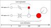 |
Fig. 1 Illustration of the follow-up of the local reionization histories for two HII regions. The red circles symbolize that the HII regions undergoe a major-merger event with another region larger or equal in volume. |
4. Evolution of lifetimes and final volumes of local reionizations
First, we present the results that were directly extracted from the simulations. We only focus on the evolution of the lifetime of the HII regions before their first major merger and their volume at this moment.
4.1. Lifetime and volume before the first major merger
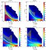 |
Fig. 2 In the background we show the distribution of the lifetime of the ionized regions before their first major merger as a function of the appearance time of the regions. The color code is in arbitrary units with blue values indicating a faint probability, while the red tones denote a high probability. The white curve represents the evolution of the mean value of the whole distribution, the shaded area stands for the 3σ uncertainty on this value. The dotted white line represents the best fit of the mean value according to the fitting formula described in Appendix A. Red, green, and yellow curves represent the same evolution for three classes of inner halo mass according to Table 2 (in solar masses for H200/S200 red: 109 − 1010, green: 1010−1011, yellow: >1011, and for H50/S50 red: 108 −109, green: 109−1010, yellow: >1010. |
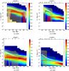 |
Fig. 3 In the background we show the volume distribution of the ionized regions before their first major merger as a function of the appearance time of the regions. The color code is in arbitrary units with blue values indicating a faint probability, while the red tones denote a high probability. The white curve represents the evolution of the mean value of the whole distribution, the shaded area stands for the 3σ uncertainty on this value. The dotted white line represents the best fit of the mean value according to the fitting formula described in Appendix A. Red, green, and yellow curves represent the same evolution for three classes of inner halo mass according to Table 2 (in solar masses for H200/S200 red: 109−1010, green: 1010 −1011, yellow: >1011, and for H50/S50 red: 108 −109, green: 109−1010, yellow: >1010. |
Figure 2 presents the evolution of the distribution of the lifetime tlife of the HII regions before their first major merger as a function of their cosmic time of appearance tapp. Figure 3 presents the same evolution for the volume of the HII regions before their first major merger. It shows the largest possible extent of the local HII region growth around sources. In both figures, the white curves represent the evolution of the distribution average and the white shaded region stands for the 3σ uncertainty on this average.
It is reassuring to note first that the same global (and expected) evolution for the distribution is found in all simulations: tlife decreases steadily with time. This drop is accompanied by a similar decrease in volume in all models. This is naturally explained by considering that as time passes a smaller volume remains neutral in the Universe. Thus, for the new regions emerging in the late phase of the reionization, the proximity effect with older regions is accentuated. Their life duration is thus naturally shorter than for early regions that appeared in a mostly neutral environment, and, moreover their growth becomes more limited.
4.1.1. Global evolution
We first compare the source models (H50 versus S50 or H200 versus S200): for the two box sizes, we note that the mean curves are very similar from one ionizing source model to another. At face value, this similarity between the two ionizing source models is surprising considering the differences in the number of sources involved from one model to another. Indeed, we would expect to find shorter lifetimes in the halo models because there are more ionizing sources than in the star models. This should promote proximity between the ionizing sites and thus encourage more rapid mergers between HII regions than in star models if we assume that the regions grow at the same rate in the two models. But the models were tailored to provide similar global reionization histories, and therefore a similar number of total emitted photons is shared among a greater number of halos than in star-based models. Therefore we may expect slower I-fronts in H simulations, and in the final volumes in Fig. 3 the H models tend to present smaller pre-merging regions than their S models counterparts: sources that are individually weaker in H simulations produce smaller ionized patches, with a slower I-front to produce similar isolation durations. Furthermore, the oldest regions (with the shortest tapp) present similar volumes before the major merger in the two models (respectively ~104 and ~102Mpc3/ h for the 200/50 Mpc/h box sizes). At the earliest times, regions grow in the same manner (duration and volume) regardless of the model taht is considered. This might imply that a good match between self-consistent stars and halos exists at this epoch, where the rarest events in the density field lead to the first emitters and are less prone to numerical subsampling.
We now compare different box sizes while considering a single ionizing source model (H50 versus H200 or S50 versus S200). The regions that appear first have a longer lifetime at low resolution (200 Mpc/h) than at high resolution (50 Mpc/h). For the oldest regions, lifetimes of ~250−200 Myr can be measured in S200 and S50 and ~300−200 Myr for H200/H50. Moreover, the slope of the mean curve is stronger in low-resolution than in high-resolution models. The combination of these two facts suggests that the oldest large regions would impose a strong UV background more suddenly in low-resolution than in high-resolution models. Indeed, when considering Fig. 3, the final volumes of these primeval bubbles are larger in large simulations and are also larger in terms of fraction of the total volume. Large volumes produce large initial reionized patches that rapidly occupy a significant fraction of the volume and prevent the rise of larger and more persistent HII regions than in the smaller boxes. This might be related to the fact that S50 and H50 simulations are too small to have a good representation of rare events and therefore cannot produce the large, initial patches that drive the subsequent percolation process and that set the duration and size of subsequent isolated HII regions. Therefore, H50/S50 simulations present a quasi-steady decline of tlife, and from one new region generation to the next there is no sudden difference in their lifetime. The duration of the local reionization histories in smaller boxes is more stable.
4.1.2. Mass dependence of local reionizations
In Figs. 2 and 3, we also decomposed the distribution into three subdistributions depending on the mass Mf of the most massive halo enclosed inside the HII region at the moment of their first major merger. The families are defined differently regarding the box size, and the family properties are summarized in Table 2. The mean curves of the three subdistributions at the one sigma level are shown for the types I, II, and III of Table 2.
First we note that in every model or box size, each class of mass occupies a specific location in the distributions. The larger the mass inside the region before its first major merger, the longer its lifetime tlife. This tendency is weaker in the S200 model because of the lack of statistics compared with others models, which results in overlapping uncertainties. Furthermore, merging HII regions with large inner mass appear among the earliest regions and cannot appear after a given cosmic time. If we consider volumes, HII regions with massive halos produce large isolated regions. Overall, this behavior is expected: HII regions with large halos when they merge enclose objects that had sufficient time (i.e., long tlife) to accrete matter in large quantities. Of course, long tlife are more easily obtained at early times when the ionization filling factor is still moderate. Conversely, regions with limited lifetimes end up with small inner halos at merging and can pretty much appear at any time during the reionization because they are likely to produce small ionized patches.
However, it can be noted that the separate evolution of the different classes of mass can be quite different from the average behaviors, especially in H models, and to some extent in S50 as well. For instance, the evolution of the average tlife is more abrupt than any of the evolutions in individual classes of mass. In terms of volumes, the same discrepancy can be noted. In these cases, the evolution of the average value is more closely related to the successive dominance of massive, intermediate, and small inner halos. Because the evolutions in durations and final volumes are weaker than globally, these models show that a merging HII region of a given size contains a well constrained mass and a given range of durations. It also implies that a merging ionized patch arose within a limited range of redshifts.
Bins of dark matter halo masses at the moment of the major merger for the three HII region families.
5. Local reionization histories as seen at z = 0
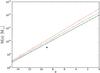 |
Fig. 4 Example of dark matter halo growth calculated according to the model of Wechsler et al. (2002) (Eq. (2)) with the fits of McBride et al. (2009). Black, green, and red curves represent the mass evolution of a MW-type halo with M0 = 1 × 10¹² M⊙ as in Battaglia et al. (2005), a M31 halo with M0 = 1.6 × 10¹² M⊙ as in Klypin et al. (2002), and an object that will have the mass our Local Group of galaxies today: M0 ~ 3 × 10¹² M⊙ as in Klypin et al. (2002). For comparison, the blue dot stands for the mass of an MW-type halo at z = 9 as found in numerical simulation by Iliev et al. (2011). |
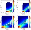 |
Fig. 5 In the background we show the duration distribution of the initial HII region growth tlife for a halo of current M0 mass, extrapolated from the value when the HII region experienced a major merger. The color code is in arbitrary units with blue values indicating a faint probability, while the red tones denote a high probability. The white curve represents the mean value evolution of the whole distribution, the shaded area stands for the 3σ uncertainty on this value. The dotted white line represents the best fit of the mean value according to the fitting formula described in Appendix B. In black we plot the same average relation, extrapolating the halo mass from the moment the HII region appears. |
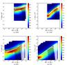 |
Fig. 6 In the background we show the volume distribution of the initial HII region growth V for a halo of current M0 mass, extrapolated from the value when the HII region experienced a major merger. The color code is in arbitrary units with blue values indicating a faint probability, while the red tones denote a high probability. The white curve represents the mean value evolution of the whole distribution, the shaded area stands for the 3σ uncertainty on this value. The dotted white line represents the best fit of the mean value according to the fitting formula described in Appendix B. In black we plot the same average relation, extrapolating the halo mass from the moment the HII region appears. |
Knowing the duration and extent of local reionizations at z > 6, we now aim at extrapolating this knowledge to z = 0 objects to gain some insights into the past local reionization history of the galaxies observed today. For this purpose we computed the mass enclosed within HII regions during the reionization epoch and extrapolated this mass from fitted halo growth relations. Ideally, this mass would have been obtained by running the hydrodynamical simulations down to z = 0, but this procedure is unfeasible at our working resolution. Details are provided in the next section, but in summary, we used the one-parameter functional form of Wechsler et al. (2002) and obtained relations such as tlife(M0) and V(M0).
5.1. Computing the mass content M0 inside the regions at z = 0
We used the one-parameter function of Wechsler et al.
(2002), 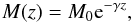 (2)which links the
mass M(z) at redshift z with the mass
M0 of the halo at redshift z = 0. The parameter
γ has the
following expressions:
(2)which links the
mass M(z) at redshift z with the mass
M0 of the halo at redshift z = 0. The parameter
γ has the
following expressions:  (3)where zf is another
parameter that corresponds to the redshift where the halo had half of its actual mass
M(zf) =
M0/ 2. We used the
simulation fits of McBride et al. (2009) where the
mean ⟨ zf
⟩ has the following expression:
(3)where zf is another
parameter that corresponds to the redshift where the halo had half of its actual mass
M(zf) =
M0/ 2. We used the
simulation fits of McBride et al. (2009) where the
mean ⟨ zf
⟩ has the following expression:
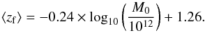 (4)To derive the mass
M0 for each HII regions we have to find
the root of the following expression:
(4)To derive the mass
M0 for each HII regions we have to find
the root of the following expression:  (5)with
M(z) being the mass at a given
redshift z
that we can access in every snapshot of the simulations thanks to the catalog.
(5)with
M(z) being the mass at a given
redshift z
that we can access in every snapshot of the simulations thanks to the catalog.
Several choices of M(z) are possible, and ideally, it would not make any difference, but in practice the individual halo growth history differ from the average behavior: the evolution of the halo mass between the appearance and the absorption of the HII region may not follow the model used here. An obvious choice would be the mass of the halo enclosed inside an HII region as it appears in the simulation. However, an HII regions appears approximately at the same time as the halo that hosted its driving source, and consequently, the halos at this moment have a mass close to the FOF detection threshold (ten particles): being light in terms of particles their mass is not accurate and can even result in HII regions devoid of inner halos because their detection is not reliable. Another choice is to consider the halo mass when the surrounding HII region merges with its neighbors (i.e., when t = tapp + tlife). At this later stage of halo buildup, masses are larger and more accurate. We chose to use this “final” mass Mf as an input to Eq. (5), even though we also considered the less reliable mass at the HII region appearance as a check. Finally, more than one halo can be contained inside the HII region: we decided to take the mass of the most massive object within an HII region as a realistic guess of the main driver of its growth.
In Fig. 4 we represent the evolution of the dark matter halo mass calculated with Eq. (2) for three halos with M0 = 1 × 10¹², M0 = 1.6 × 10¹², and M0 ~ 3 × 10¹² M⊙ that correspond to an MW-type halo (see Battaglia et al. 2005), an M31-type one, and to an object that would have the mass of the Local Group at z = 0 (see Klypin et al. 2002). For comparison we show the result found for the mass of an MW-type halo at z = 9 in a numerical simulation (see Iliev et al. 2011). The model of Wechsler et al. (2002) leads to a difference of a factor of ~2 with the results of the simulation. We even obtain a good order of magnitude and stress that the following results are obviously model dependant and need simulation results at z = 0 to be more precise.
In the following we present a trend of the of galaxy reionization histories observed today, taking into account that our quantitative results are prone to variations. From the relations detailed above, and for each HII region with tlife and V as it merges, we compute the tlife(M0) and V(M0) at z = 0.
5.2. Lifetime and volume as a function of M(z = 0) = M0
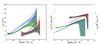 |
Fig. 7 Average duration (left) and largest expansion (right) of the initial HII region growth as a function of the mass of the most massive halo extrapolated at z = 0. Black and red curves stand for the star-based and halo-based model in the 200 Mpc/h simulation. Green and blue stand for the star-based and halo-based model in the 50 Mpc/h simulation. Shaded areas stand for the 3σ error on the average value. |
We present the evolution tlife(M0) of the region lifetime before their major merger as a function of M0 in Fig. 5. Figure 6 shows the final volume of an isolated HII region as a function of the current mass, V(M0). For comparison, all the models are superimposed in Fig. 7 for both tlife(M0) and V(M0).
Comparing the source models for a fixed resolution (i.e., S50 vs. H50 or S200 vs. H200), the same trends can be observed. At large M0, the final volume of the HII regions does not depend on the model. This convergence is achieved for M0> 1013 M⊙ in the 200 Mpc/h simulations and M0> 1011 M⊙ in the 50 Mpc/h simulations. In terms of isolation duration (tlife), the same objects will nevertheless differ: halo-based models tend to produce a longer local reionization than star-based models. Low-mass objects follow a quite different trend: halo-based model tend to surround these objects with smaller HII regions than star-based models, and at the same time the differences in duration of local reionizations tend to be reduced. We recall that emissivities were tailored to have both models that produce the same global reionization history and therefore similar photon production histories. Let us also recall that halo models provide more sources than star-based models: as a consequence, fewer photons are cast per halo at a given resolution. For large-mass objects, the final volume does not depend on the source model, which suggests that large HII regions are spatially distributed in the same manner in both descriptions. At the same time, emissivities are lower in H models, which leads to a slower propagation of I-fronts than in S calculations. For low-mass objects, the situation is slightly different: H models present many small and clustered HII regions, induced by small halos during the reionization which translates into small objects at z = 0. Therefore the final volumes are smaller than in star-based models, compensate for the lower emissivities per source, and reduce the difference in terms of duration of local reionizations. These differences between H and S models were already present in the merger-tree and radii statistics in Chardin et al. (2012), and the results obtained here are another view of the impact of source modeling on the geometry of HII regions during the reionization.
Decreasing the simulated volume typically leads to a decrease in HII region volumes and prolongs the expansion duration of HII regions. Again, increasing the resolution increases the number of sources for both models and therefore decreases the photon-production rate per source. The higher density of sources naturally reduces the volume available for an HII region, and to have similar global reionization histories in the 50 and 200 Mpc/h simulations, the expansion rate of HII regions must be reduced in the 50 Mpc/h experiments. Quantitatively, the final volumes are one order of magnitude larger in the 200 Mpc/h simulations, with typical radii of 5.2 Mpc/h for the HII regions before they merge for 1013 M⊙ haloes compared with 1.7 Mpc/h in the 50 Mpc/h experiments. For the least massive halos within the 50 Mpc/h simulation (M0 ~ 1.5 × 10⁹ M⊙), their radii can be as small as 150 kpc/h in the H50 model and 350 kpc/h in the S50 model. The difference is greater for low-mass objects in the larger box, with typical radii of 1.3 Mpc/h in H200 for M0 ~ 2 × 10¹¹ M⊙ and 4 Mpc/h in S200. In terms of duration, tlife increases from 70 Myr to 250 Myr in the 50 Mpc/h experiments and from 70 to ~200 Myr in the 200 Mpc/h, but over a range of larger masses. Globally, the two models agree better in the small box, which was seen previously in the merger-tree statistics of Chardin et al. (2012). For the dispersion in the value distributions in the backgrounds of Figs. 5 and 6, the scatter is still quite large in all situations, and the differences noted above lie in the range of values that are allowed by this dispersion.
Regardless of the model or resolution considered, the properties of the initial growth are strongly mass dependent. The most massive objects seen today grow from the earliest progenitors with an accretion rate then at the highest levels and a longer accretion history. In addition, the initial growth stages of their HII regions occurred within a mostly neutral Universe. Combined with the fact that they are strong emitters, it is thus expected that their HII regions dominate for a long time before they merged into a larger UV background. In our models 300 Myr represents approximately one third of the reionization epoch, which is a significant fraction that corresponds to several dynamical times at this epoch or a few generations of massive stars. Taking M0 = 1012 M⊙ as an example and depending on the box-size/model used to constrain these values, such a halo would have reionized a radius of 2.9 ± 1.6 Mpc/h after a period of between 50 and 200 Myr. This implies that for this duration these objects experience inside-out reionization with properties decoupled from a cosmic average behavior, with local anisotropies or inhomogeneities for instance. At the low-mass end of the mass range explored here, the associated HII regions are merged into the UV background after a few tens of Myr, resulting both from environmental effects where close larger regions dominate and from the fact that these objects appear at the latest stages of reionization where the ionized filling fraction is close to one. These low-mass objects experienced a reionization that is more in line with the commonly picture of an object that is rapidly part of a uniform UV background. Overall, it is clear that depending on the mass (which is related to a variety of environments or a variety of internal histories of source buildup) a broad variety of local reionization histories are possible, quite different from the homogeneous rise of a global UV flux.
Finally, we show in the same figures the relations obtained using a different procedure to compute the current mass M0: instead of using the mass of the most massive halos as the HII region merge in the halo growth model, we used the same mass, but when the HII region appeared. The relations are shown in black in Figs. 5 and 6. Clearly, it does not really make a significant difference, with trends and quantitative values consistent with the other choice of initial mass. The strongest impact is on massive halos, which is expected: they appear at the earliest time, therefore the initial uncertainty on their mass (which is close to ten particles) is propagated and amplified over a longer time. Overall, this acts as an indirect proof that our arbitrary choice of Mf does not have a strong influence on the extrapolation.
5.3. Apparition time and merger redshift with the UV background as a function of M(z = 0) = M0
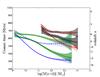 |
Fig. 8 Mean cosmic appearance time (solid lines) and mean redshift of a merger with the UV background (dashed lines) as a function of the mass of the most massive halo extrapolated at z = 0. Black and red curves stand for the star-based and halo-based model in the 200 Mpc/h simulation. Green and blue stand for the star-based and halo-based model in the 50 Mpc/h simulation. Shaded areas stand for the 3σ error on the average value. |
In Fig. 8, we show the evolution of the mean cosmic appearance time of the HII regions as a function of the mass of their progenitors extrapolated at z = 0 for our four models. It is first reassuring to note that, regardless of the model considered, the most massive haloes today are on average associated with the oldest HII regions, with the shortest appearance times. The different HII regions can appear as soon as 300 Myr after the Big Bang in the 50 Mpc/h box for the most massive halos observed at z = 0. The regions that appear last corresponding to low-mass z = 0 halos can emerge until 650 Myr in the same box. The first regions appear later in the large box of 200 Mpc/h at ~500 Myr, but the last regions emerge until ~750 Myr. These differences reflect the differences of resolutions with sources appearing earlier in the 50 Mpc/h boxes than in the 200 Mpc/h experiments, where sources appear later, but can reach higher values of appearance in cosmic time to complete the reionization.
In the same figure, we also show the evolution of the mean cosmic merger time (redshift) with the UV background for the halos as a function of their mass at z = 0. Surprinsingly, we observe a sort of “plateau” in all the models for the reionization redshift for a certain range of M0 halos. Indeed, an almost constant redshift of z ~ 8−9 is observed in the 200 and 50 Mpc/h boxes for halos with M0> 1 × 10¹² M⊙. These redshifts correspond to the beginning of the intense merger period of the HII regions and to the emergence of a main HII region in size, as noted in Chardin et al. (2012). It thus seems that halos with M0> 1 × 10¹² M⊙ initiated their buildup before that period, that their associated HII regions dominated the merging process, and that, on average, they completed their isolated reionization history at the intense overlap epoch regardless of their appearance time.
Halos with M0< 1 × 10¹² M⊙ on average initiated their buildup during or after this merger period and thus in an already significantly ionized environment. We observe that the lower the mass of the halos, the later they reache the reionization, with a difference between their lifetime and appearance time that decreases. This is expected as soon as the low-mass halos are those that appeared later with an enhanced proximity effect with other HII regions.
6. Discussion
6.1. Convergence problems
The previous results highlight one important fact: the difficulty to reach convergence between the two ionizing source models at both resolutions. Despite the certain degree of similaritiy reported in Chardin et al. (2012, Paper I) between the two models, only the same global behavior can be observed. All the ionizing source models and resolution studies agree on the fact that the most massive z = 0 haloes have expanding HII regions during a much longer time and thus fill in a much larger volume than low-mass objects before they are incorporated into the UV background. However, the quantitative results still disagree and are extremely model and resolution dependent. Nevertheless, we show here that some halo mass ranges exist, depending on the resolution, where our results converge for both ionizig source models. The main problem with our quantitative results shown in the next is the advantages and drawbacks concerning the two resolution cases studied. Indeed, the 200 Mpc/h box has the advantage of resolving the rare density peak, thus accounting for cosmic variance effect and allowing us to track the largest HII regions. In contrast, the 50 Mpc/h box has a better resolution than its 200 Mpc/h analog and can thus resolve smaller HII regions and account for the inhomogeneity of the reionization process. We have to keep these aspects in my mind when we interpret our results in the next section.
In Paper I, we noted that both ionizing source prescriptions lead to a similar evolution for the radius distribution of HII regions with redshift and for their merger history. It thus appears that the star-based model could be able to reproduce at a certain level a similar morphology of the reionization process than the one provided by halo sources. With the present study this affirmation seems to loose some degree of validity when extrapolating the results from high-z to z = 0.
More precisely, we found in Paper I (Fig. 11) a cut-off radius (0.4 Mpc/h, (4 Mpc/h) in the 50 Mpc/h model, (200 Mpc/h model)) in the evolution with redshift of the radius distribution of HII regions. Above this radius cut-off, the radius distribution of the star prescription becomes the analog of the one provided by the halo sources. In the V(M0) evolution of Fig. 7, we therefore have a higher reliability of the results in the range of volumes above these cut-offs at both resolutions. This is the volume range where we argue that our results converge for both ionizing source prescriptions. At both resolutions these “converged” volume ranges can translate into z = 0 halo mass range. Indeed, we can consider only the mass range where both V(M0) curves corresponding to the two ionizing source models exceed the cut-off radius. Therefore the mass ranges for which we are the most confident regarding our results are for haloes with mass M ≥ 1 × 10¹³ M⊙, (M ≥ 1 × 10¹¹ M⊙) in the 200 Mpc/h box, (50 Mpc/h box).
In the present paper, when we consider the V(M0) evolution for the mass range of confidence, we can note that the convergence in the reionized volume by the haloes is still present between both ionizing source models: the evolution of the HII region sizes becomes almost superimposed in the two ionizing source model at both resolutions. In other words, the convergence seen at high z for the HII region sizes is translated at z = 0. However, it seems that differences appear in the tlife(M0) between the two models at both resolutions. In the two-resolution cases, a difference of ~50 Myr in the isolated reionization history duration is observed almost throughout the halo mass ranges of confidence. For example, a halo with a mass of ~1 × 10¹³ M⊙ has a tlife ~ 100−150 Myr for the star and halo model in the 200 Mpc/h experiments and a tlife ~ 200−250 Myr in the 50 Mpc/h simulations. This gap again reflects the difference between the emissivity of the two models with a high number of haloes casting a smaller number of ionizing photons than the stronger star emitters needed to counterbalance their smaller number. In other words, we observe a memory effect of the differences generated by the emissivity models that are still present in the z = 0 results.
6.2. Predictions for the Local Group
In the 200 Mpc/h simulations, the halo mass range for which we achieve a good convergence level between the two models begins with too high masses (above ~1013 M⊙) to make strong predictions about the past reionization history of peculiar galaxies such as the Milky Way with a halo mass of ~1012 M⊙ (see Battaglia et al. 2005). However, in the 50 Mpc/h experiment, we obtain a reasonable degree of convergence between the simulation for halos with mass M ≥ × 1011 M⊙. At this resolution, 1012 M⊙ haloes have reionization times of ~150 ± 15 Myr or ~200 ± 15 Myr in the star and halo prescriptions and a typical radius of ~1.1 Mpc/h for the HII region. Recently, Li et al. (2014) assessed the reionization history of Milky Way-type halos. They found median reionization times of ~115 Myr for a halo mass of 1 × 10¹² M⊙ which is a slightly shorter than our averaged estimate. But they used median values that might be close to our results because our averaged value is higher than the median estimate we derived. On the other hand, radiative transfer simulations of the Local Group of Ocvirk et al. (2013), post-processed on the CLUES simulation (see Libeskind et al. 2010), produced isolated reionizations of the Milky Way (M ~ 3 × 10¹¹ M⊙ ) with times of 130 Myr in their photon-rich H43 model (the closest to our emissivity model), with a maximal extension of ~1 Mpc/h for the corresponding HII region. For the same halo mass, we found ~135 ± 10 and ~175 ± 10 Myr for the star and halo models with a typical radius of ~0.7 Mpc/h, which is close to their results. Therefore, our statistical sample of reionization histories could be representative of the particular case of the MW reionization history.
In Fig. 9 we present an illustration of the reionization process of Local Group-type objects as suggested by our results. For a halo of ~3 × 10¹² M⊙ (see Klypin et al. 2002) with a mass similar to that of the whole Local Group (composed of MW and M31), our results indicate a possible HII region extension with a radius of ~1.5 Mpc/h (still in the 50 Mpc/h box) before encountering another front. In other words, a volume just large enough to encompass the whole Local Group. Statistically, a halo with a mass similar to that of the Local Group could therefore have been able to reionize by itself and not be swept up by the radiation of a Virgo-like close cluster.
However, the Local Group could also have been reionized by dwarf galaxies instead of by their central lighthouse, according to large-scale simulations of cosmic reionization (see Iliev et al. 2007; Salvaterra et al. 2011; Kuhlen & Faucher-Giguère 2012; Mitra et al. 2013). These studies suggest that haloes that would form the dwarf galaxies with total masses M ≤ 109 M⊙ could provide a significant fraction of the ionizing photon budget during cosmic reionization (Wise et al. 2014). Cosmic reionization could indeed have been primarily driven by protogalaxies in haloes with masses between 107 M⊙ and 108 M⊙, which have very high escape fractions (Paardekooper et al. 2013). Moreover, Salvadori et al. (2014) suggest that dwarf galaxies with M ≤ 109 M⊙ could provide a significant fraction of the ionizing photon budget during cosmic reionization and that M ≤ 109 M⊙ dwarf galaxies could have dominated the reionization of galaxies like our own Milky Way, providing >80% of the required photon budget. Unfortunately, we lacked the resolution to track such dwarf galaxies. Nevertheless, the recent studies of Ocvirk et al. (2013) suggest alternatively that the reionization of the Local Group could have been driven in an inside-out way under the influence of the central main halos. In summary, the answer to the question of an internal versus external reionization history of MW-type galaxies could be tested with higher resolution large-scale simulations of the Local Group.
Finally, as argued before, we emphasize that the 50 Mpc/h simulations has the default of finite-volume effects and therefore cannot include rare density peaks or large voids that may be expected. Moreover, its volume is not large enough to track the evolution of large HII regions during the reionization. To support the results drawn from our 50 Mpc/h experiment, the ideal case would be the 200 Mpc/h simulation with the same resolution as that of the 50 Mpc/h simulation to ensure that we are insensitive to cosmic variance.
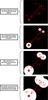 |
Fig. 9 Ilustration of the reionization of a Local Group-type object as suggested by our results. |
Linear fits for the cosmic time dependence of the mean lifetime ⟨ tlife ⟩ of a region before its first major merger and its mean volume ⟨ Volume ⟩ at this moment.
7. Summary and prospects
We investigated simple properties of the initial stage of the reionization process around progenitors of galaxies, such as the extent of the initial HII region before its absorption by the UV background, and the duration of its propagation. We investigated multiple reionization histories in a set of four simulations where we varied the ionizing source prescriptions and the simulation resolution. By using a merger tree of HII regions (here defined as regions with an ionizing fraction x ≥ 0.5), we compiled a catalog of the HII region properties for all ionized regions that appeared in the experiments. We then examined the time when the HII regions undergo a major merger event, and considered that the region is a part of the global UV background.
From the lifetimes of the regions and their volume at this moment we drew typical local reionization histories as a function of the cosmic time of appearance of the HII regions. We also investigated the link between these histories and the dark matter halo masses inside the regions. By using a motivated functional form for the average mass accretion history of the dark matter halos, we then extrapolated the mass inside the region at z = 0 to predict the past reionization histories of galaxies seen today.
Linear fits for the M0 dependence of the mean lifetime ⟨ tlife ⟩ of a region before its first major merger and its mean volume ⟨ Volume ⟩ at this moment.
Our results are summarized as follows:
-
We found that the later an HII region appears during thereionization period, the shorter will be their related lifetime andvolume before they merge with the global UV background. This isa normal consequence of the overlap of ionized patches thatreduce the neutral volume available for I-front propagation.However, quantitatively, the duration and the extent of the initialgrowth of an HII region is strongly dependent on the mass of theinner halo. During this initial stage, this can be as long as 350−400 Myr (i.e., ~50% of the reionization), thisinner halo and the galaxies it hosts are decoupled from the externalUV background.
-
We extrapolated the mass of dark matter halos at high z to z = 0 using a halo-growth model to predict the extent and duration of these initial HII regions around current galaxies. The quantitative prediction differs depending on the box size or the source model: by enforcing similar global reionization histories, small simulated volumes promote proximity effects between HII regions, and halo-based source models predict smaller regions and a slower I-front expansion.
-
From the mean reionization redshift of the galaxies as a function of M0, we found that on average, halos with M0> 1 × 10¹² M⊙ appeared during the pre-overlap period and left the isolated reionization regime at the overlap regardless of their appearance time in the cosmic history.
-
Applying this extrapolation to the Local Group leads to a typical extent of 1.1 Mpc/h for the initial HII region around a typical Milky Way that established itself in ~150–200 ± 20 Myr. This is comparable with the recent constrained simulation of the Local Group reported by Ocvirk et al. (2013) which means that our statistical study might be representative of particular galaxy ionization histories in this mass range. Considering the whole Local Group, our result suggests that statistically it should not have been influenced by an external front that originated from a Virgo-like cluster.
From the results of this study, we plan to repeat this technique on enhanced reionization simulations, the ideal situation being an experiment where at least the dark matter field evolution would be ran until z = 0. This would liberate us from the impact of any semi-analytical framework for extrapolating the mass at z = 0, and we therefore would calculate only with quantities directly generated during the simulation. Using the same methodology, we aim at expanding these measurements to the statistics of the inner properties of these local reionizations such as I-front propagation profiles or anisotropies. Ultimately, they will provide a detailed framework of the initial reionization stages around galaxies that could then be included in semi-analytical modeling or hydrodynamical simulations without radiative transfer.
Acknowledgments
The authors would like to thank Hervé Wozniak, Benoît Semelin, and Martin Haehnelt for comments and discussions. The simulations were run on the Curie Supercomputer (CCRT-CEA) using PRACE Preparatory Access time. This study was performed in the context of the EMMA (ANR-12-JS05-0001) & LIDAU (ANR-09-BLAN-0030) projects, funded by the Frensh Agence Nationale pour la Recherche (ANR).
References
- Aubert, D., & Teyssier, R. 2008, MNRAS, 387, 295 [NASA ADS] [CrossRef] [Google Scholar]
- Aubert, D., & Teyssier, R. 2010, ApJ, 724, 244 [NASA ADS] [CrossRef] [Google Scholar]
- Baek, S., Di Matteo, P., Semelin, B., Combes, F., & Revaz, Y. 2009, A&A, 495, 389 [NASA ADS] [CrossRef] [EDP Sciences] [Google Scholar]
- Battaglia, G., Helmi, A., Morrison, H., et al. 2005, MNRAS, 364, 433 [NASA ADS] [CrossRef] [Google Scholar]
- Chardin, J., Aubert, D., & Ocvirk, P. 2012, A&A, 548, A9 [NASA ADS] [CrossRef] [EDP Sciences] [Google Scholar]
- Courtin, J., Rasera, Y., Alimi, J.-M., et al. 2011, MNRAS, 410, 1911 [NASA ADS] [Google Scholar]
- Croft, R. A. C., & Altay, G. 2008, MNRAS, 388, 1501 [NASA ADS] [CrossRef] [Google Scholar]
- Fan, X., Strauss, M. A., Becker, R. H., et al. 2006, AJ, 132, 117 [NASA ADS] [CrossRef] [EDP Sciences] [Google Scholar]
- Finlator, K., Davé, R., & Özel, F. 2011, ApJ, 743, 169 [NASA ADS] [CrossRef] [Google Scholar]
- Friedrich, M. M., Mellema, G., Alvarez, M. A., Shapiro, P. R., & Iliev, I. T. 2011, MNRAS, 413, 1353 [NASA ADS] [CrossRef] [Google Scholar]
- Furlanetto, S. R., Zaldarriaga, M., & Hernquist, L. 2004, ApJ, 613, 1 [NASA ADS] [CrossRef] [Google Scholar]
- Furlanetto, S. R., McQuinn, M., & Hernquist, L. 2006, MNRAS, 365, 115 [NASA ADS] [CrossRef] [Google Scholar]
- Hasegawa, K., & Umemura, M. 2010, MNRAS, 407, 2632 [NASA ADS] [CrossRef] [Google Scholar]
- Iliev, I. T., & C. R. T. C. Collaboration 2009, Mem. Soc. Astron. It., 80, 415 [NASA ADS] [Google Scholar]
- Iliev, I. T., Ciardi, B., Alvarez, M. A., et al. 2006a, MNRAS, 371, 1057 [NASA ADS] [CrossRef] [Google Scholar]
- Iliev, I. T., Mellema, G., Pen, U., et al. 2006b, MNRAS, 369, 1625 [NASA ADS] [CrossRef] [Google Scholar]
- Iliev, I. T., Mellema, G., Shapiro, P. R., & Pen, U.-L. 2007, MNRAS, 376, 534 [NASA ADS] [CrossRef] [Google Scholar]
- Iliev, I. T., Whalen, D., Mellema, G., et al. 2009, MNRAS, 400, 1283 [NASA ADS] [CrossRef] [Google Scholar]
- Iliev, I. T., Moore, B., Gottlöber, S., et al. 2011, MNRAS, 413, 2093 [NASA ADS] [CrossRef] [Google Scholar]
- Klypin, A., Kravtsov, A. V., Valenzuela, O., & Prada, F. 1999, ApJ, 522, 82 [Google Scholar]
- Klypin, A., Zhao, H., & Somerville, R. S. 2002, ApJ, 573, 597 [Google Scholar]
- Komatsu, E., Dunkley, J., Nolta, M. R., et al. 2009, ApJS, 180, 330 [NASA ADS] [CrossRef] [Google Scholar]
- Krumholz, M. R., Klein, R. I., McKee, C. F., & Bolstad, J. 2007, ApJ, 667, 626 [NASA ADS] [CrossRef] [Google Scholar]
- Kuhlen, M., & Faucher-Giguère, C.-A. 2012, MNRAS, 423, 862 [NASA ADS] [CrossRef] [Google Scholar]
- Lacey, C., & Cole, S. 1993, MNRAS, 262, 627 [NASA ADS] [CrossRef] [Google Scholar]
- Li, T. Y., Alvarez, M. A., Wechsler, R. H., & Abel, T. 2014, ApJ, 785, 134 [NASA ADS] [CrossRef] [Google Scholar]
- Libeskind, N. I., Yepes, G., Knebe, A., et al. 2010, MNRAS, 401, 1889 [NASA ADS] [CrossRef] [Google Scholar]
- McBride, J., Fakhouri, O., & Ma, C.-P. 2009, MNRAS, 398, 1858 [NASA ADS] [CrossRef] [Google Scholar]
- McQuinn, M., Lidz, A., Zahn, O., et al. 2007, MNRAS, 377, 1043 [NASA ADS] [CrossRef] [Google Scholar]
- Mellema, G., Iliev, I. T., Pen, U.-L., & Shapiro, P. R. 2006, MNRAS, 372, 679 [NASA ADS] [CrossRef] [Google Scholar]
- Mitra, S., Ferrara, A., & Choudhury, T. R. 2013, MNRAS, 428, L1 [NASA ADS] [CrossRef] [Google Scholar]
- Moore, B., Ghigna, S., Governato, F., et al. 1999, ApJ, 524, L19 [Google Scholar]
- Ocvirk, P., & Aubert, D. 2011, MNRAS, 417, L93 [NASA ADS] [CrossRef] [Google Scholar]
- Ocvirk, P., Aubert, D., Chardin, J., et al. 2013, ApJ, 777, 51 [NASA ADS] [CrossRef] [Google Scholar]
- Paardekooper, J.-P., Khochfar, S., & Dal la Vecchia, C. 2013, MNRAS, 429, L94 [NASA ADS] [CrossRef] [Google Scholar]
- Prunet, S., Pichon, C., Aubert, D., et al. 2008, ApJS, 178, 179 [NASA ADS] [CrossRef] [Google Scholar]
- Rasera, Y., & Teyssier, R. 2006, A&A, 445, 1 [NASA ADS] [CrossRef] [EDP Sciences] [Google Scholar]
- Roukema, B. F., & Yoshii, Y. 1993, ApJ, 418, L1 [NASA ADS] [CrossRef] [Google Scholar]
- Roukema, B. F., Quinn, P. J., & Peterson, B. A. 1993, in Observational Cosmology, eds. G. L. Chincarini, A. Iovino, T. Maccacaro, & D. Maccagni, ASP Conf. Ser., 51, 298 [Google Scholar]
- Roukema, B. F., Quinn, P. J., Peterson, B. A., & Rocca-Volmerange, B. 1997, MNRAS, 292, 835 [NASA ADS] [CrossRef] [Google Scholar]
- Salvadori, S., Tolstoy, E., Ferrara, A., & Zaroubi, S. 2014, MNRAS, 437, L26 [NASA ADS] [CrossRef] [Google Scholar]
- Salvaterra, R., Ferrara, A., & Dayal, P. 2011, MNRAS, 414, 847 [NASA ADS] [CrossRef] [Google Scholar]
- Shin, M., Trac, H., & Cen, R. 2008, ApJ, 681, 756 [NASA ADS] [CrossRef] [Google Scholar]
- Wechsler, R. H., Bullock, J. S., Primack, J. R., Kravtsov, A. V., & Dekel, A. 2002, ApJ, 568, 52 [NASA ADS] [CrossRef] [Google Scholar]
- Willott, C. J., Delorme, P., Omont, A., et al. 2007, AJ, 134, 2435 [NASA ADS] [CrossRef] [Google Scholar]
- Wise, J. H., & Abel, T. 2011, MNRAS, 414, 3458 [NASA ADS] [CrossRef] [Google Scholar]
- Wise, J. H., Demchenko, V. G., Halicek, M. T., et al. 2014, MNRAS, 442, 2560 [NASA ADS] [CrossRef] [Google Scholar]
- Zahn, O., Lidz, A., McQuinn, M., et al. 2007, ApJ, 654, 12 [NASA ADS] [CrossRef] [Google Scholar]
Appendix A: Fitting models
To approximate the cosmic time dependence of the mean lifetime of the HII regions, we
used the two-parameter exponential form,
 (A.1)In Table A.1 we summarize the best-fit parameters for the mean
curve of the complete distribution for each simulation. We present the best fits of the
curves in Fig. 2 with the dotted white line.
(A.1)In Table A.1 we summarize the best-fit parameters for the mean
curve of the complete distribution for each simulation. We present the best fits of the
curves in Fig. 2 with the dotted white line.
To approximate the cosmic time dependence of the mean volume of the HII regions at the
moment of the major merger, we the used two-parameter exponential form,
 (A.2)We report in Table A.1 the best-fit coefficients found in every model and
also give the mean dispersion along the curve. The best fits of the curves are shown in
Fig. 3 with the dotted white line. These fits might
be useful to assign a typical volume for the HII regions as a function of cosmic time.
(A.2)We report in Table A.1 the best-fit coefficients found in every model and
also give the mean dispersion along the curve. The best fits of the curves are shown in
Fig. 3 with the dotted white line. These fits might
be useful to assign a typical volume for the HII regions as a function of cosmic time.
Appendix B: Fitting models at z = 0
To approximate the M0 dependence of the mean lifetime of
the HII regions, we used the two-parameter form,  (B.1)In Table B.1 we summarize the best-fit parameters for the mean
curve of the complete distribution for each simulation. We present the best-fits of the
curve in Fig. 5 with the dotted white line.
(B.1)In Table B.1 we summarize the best-fit parameters for the mean
curve of the complete distribution for each simulation. We present the best-fits of the
curve in Fig. 5 with the dotted white line.
To approximate the M0 dependence of the mean volume of the
HII regions at the moment of the major merger, we used the two-parameter form,
 (B.2)We report in Table
B.1 the best-fit coefficients found in every
model and also give the mean dispersion along the curve. The best fits of the curves are
shown in Fig. 6 with the dotted white line. These
fits might be useful to assign typical volume for the HII regions as a function of cosmic
time.
(B.2)We report in Table
B.1 the best-fit coefficients found in every
model and also give the mean dispersion along the curve. The best fits of the curves are
shown in Fig. 6 with the dotted white line. These
fits might be useful to assign typical volume for the HII regions as a function of cosmic
time.
All Tables
Bins of dark matter halo masses at the moment of the major merger for the three HII region families.
Linear fits for the cosmic time dependence of the mean lifetime ⟨ tlife ⟩ of a region before its first major merger and its mean volume ⟨ Volume ⟩ at this moment.
Linear fits for the M0 dependence of the mean lifetime ⟨ tlife ⟩ of a region before its first major merger and its mean volume ⟨ Volume ⟩ at this moment.
All Figures
|
Fig. 1 Illustration of the follow-up of the local reionization histories for two HII regions. The red circles symbolize that the HII regions undergoe a major-merger event with another region larger or equal in volume. |
| In the text | |
|
Fig. 2 In the background we show the distribution of the lifetime of the ionized regions before their first major merger as a function of the appearance time of the regions. The color code is in arbitrary units with blue values indicating a faint probability, while the red tones denote a high probability. The white curve represents the evolution of the mean value of the whole distribution, the shaded area stands for the 3σ uncertainty on this value. The dotted white line represents the best fit of the mean value according to the fitting formula described in Appendix A. Red, green, and yellow curves represent the same evolution for three classes of inner halo mass according to Table 2 (in solar masses for H200/S200 red: 109 − 1010, green: 1010−1011, yellow: >1011, and for H50/S50 red: 108 −109, green: 109−1010, yellow: >1010. |
| In the text | |
|
Fig. 3 In the background we show the volume distribution of the ionized regions before their first major merger as a function of the appearance time of the regions. The color code is in arbitrary units with blue values indicating a faint probability, while the red tones denote a high probability. The white curve represents the evolution of the mean value of the whole distribution, the shaded area stands for the 3σ uncertainty on this value. The dotted white line represents the best fit of the mean value according to the fitting formula described in Appendix A. Red, green, and yellow curves represent the same evolution for three classes of inner halo mass according to Table 2 (in solar masses for H200/S200 red: 109−1010, green: 1010 −1011, yellow: >1011, and for H50/S50 red: 108 −109, green: 109−1010, yellow: >1010. |
| In the text | |
|
Fig. 4 Example of dark matter halo growth calculated according to the model of Wechsler et al. (2002) (Eq. (2)) with the fits of McBride et al. (2009). Black, green, and red curves represent the mass evolution of a MW-type halo with M0 = 1 × 10¹² M⊙ as in Battaglia et al. (2005), a M31 halo with M0 = 1.6 × 10¹² M⊙ as in Klypin et al. (2002), and an object that will have the mass our Local Group of galaxies today: M0 ~ 3 × 10¹² M⊙ as in Klypin et al. (2002). For comparison, the blue dot stands for the mass of an MW-type halo at z = 9 as found in numerical simulation by Iliev et al. (2011). |
| In the text | |
|
Fig. 5 In the background we show the duration distribution of the initial HII region growth tlife for a halo of current M0 mass, extrapolated from the value when the HII region experienced a major merger. The color code is in arbitrary units with blue values indicating a faint probability, while the red tones denote a high probability. The white curve represents the mean value evolution of the whole distribution, the shaded area stands for the 3σ uncertainty on this value. The dotted white line represents the best fit of the mean value according to the fitting formula described in Appendix B. In black we plot the same average relation, extrapolating the halo mass from the moment the HII region appears. |
| In the text | |
|
Fig. 6 In the background we show the volume distribution of the initial HII region growth V for a halo of current M0 mass, extrapolated from the value when the HII region experienced a major merger. The color code is in arbitrary units with blue values indicating a faint probability, while the red tones denote a high probability. The white curve represents the mean value evolution of the whole distribution, the shaded area stands for the 3σ uncertainty on this value. The dotted white line represents the best fit of the mean value according to the fitting formula described in Appendix B. In black we plot the same average relation, extrapolating the halo mass from the moment the HII region appears. |
| In the text | |
|
Fig. 7 Average duration (left) and largest expansion (right) of the initial HII region growth as a function of the mass of the most massive halo extrapolated at z = 0. Black and red curves stand for the star-based and halo-based model in the 200 Mpc/h simulation. Green and blue stand for the star-based and halo-based model in the 50 Mpc/h simulation. Shaded areas stand for the 3σ error on the average value. |
| In the text | |
|
Fig. 8 Mean cosmic appearance time (solid lines) and mean redshift of a merger with the UV background (dashed lines) as a function of the mass of the most massive halo extrapolated at z = 0. Black and red curves stand for the star-based and halo-based model in the 200 Mpc/h simulation. Green and blue stand for the star-based and halo-based model in the 50 Mpc/h simulation. Shaded areas stand for the 3σ error on the average value. |
| In the text | |
|
Fig. 9 Ilustration of the reionization of a Local Group-type object as suggested by our results. |
| In the text | |
Current usage metrics show cumulative count of Article Views (full-text article views including HTML views, PDF and ePub downloads, according to the available data) and Abstracts Views on Vision4Press platform.
Data correspond to usage on the plateform after 2015. The current usage metrics is available 48-96 hours after online publication and is updated daily on week days.
Initial download of the metrics may take a while.