| Issue |
A&A
Volume 567, July 2014
|
|
|---|---|---|
| Article Number | A114 | |
| Number of page(s) | 16 | |
| Section | Astrophysical processes | |
| DOI | https://doi.org/10.1051/0004-6361/201323140 | |
| Published online | 24 July 2014 | |
Photonic orbital angular momentum in starlight⋆
Further analysis of the 2011 Starfire Optical Range Observations
1
Leidos,
Albuquerque
New Mexico,
USA
e-mail:
This email address is being protected from spambots. You need JavaScript enabled to view it.
2
Air Force Research Laboratory, Directed Energy Directorate, Kirtland AFB, New Mexico, USA
Received:
27
November
2013
Accepted:
8
June
2014
Abstract
Context. Each attempt by the Atmospheric Simulation and Adaptive-optics Laboratory Testbed (ASALT) research group to detect turbulence-induced photonic orbital angular momentum (POAM) has been successful, spanning laboratory, simulation and field experiments, with the possible exception of the 2011 Starfire Optical Range (SOR) astronomical observations, a search for POAM induced by astronomical sources.
Aims. The purposes of this work are to discuss how POAM from astronomical turbulent assemblages of molecules or atoms (TAMA) would appear in observations and then to reanalyze the data from the 2011 SOR observations using a more refined technique as a demonstration of POAM in starlight.
Methods. This work uses the method of projections used previously in analysis of terrestrial data.
Results. Using the method of projections, the noise floor of the system was reevaluated and is found to be no greater than 1%. Reevaluation of the 2011 SOR observations reveals that a POAM signal is evident in all of the data.
Conclusions. POAM signals have been found in every instance of extended propagation through turbulence conducted by the ASALT research group, including the 2011 SOR observations. POAM is an inevitable result of the propagation of optical waves through turbulence.
Key words: ISM: general
We express our gratitude to the Air Force Office of Scientific Research for their support of this research.
© ESO, 2014
1. Introduction
Photonic orbital angular momentum (POAM), the fifth property of light, may be of significant interest to the astronomical community (Harwit 2003; Elias 2008). Since the discovery by Allen et al. (1992) that POAM can be easily created in the laboratory, it has been found in virtually every field of optics Yao & Padgett (2011); Tamburini et al. (2012); Shalaev et al. (2013); Kim et al. (2013); Chen et al. (2013); Cristi & Axtell (2013); Sun et al. (2013); Ruane & Swatzlander (2013); Roux (2013); this ubiquity is evident in the more than 1000 papers citing the original work (Allen et al. 1992). The demonstration that POAM is a natural consequence of the interaction of light and turbulence (Sanchez & Oesch 2011a,b; Oesch & Sanchez 2012; Oesch et al. 2013), provides a mechanism by which POAM may be created in large quantities by astrophysical systems. Sanchez et al. (2013) explained this mechanism in the context of astronomical turbulence along with a survey of the POAM signal from five stars using the 3.5 m telescope and natural guide star wavefront sensor (WFS) at the Starfire Optical Range (SOR). The original survey stars: 49 Ceti, HR 1784, HR 1529, HR 1577 and HR 1895, were chosen primarily based on their altitude and brightness at the time of the observations, but two of these candidate stars were chosen because of their known association with a turbulent assemblage of molecules or atoms (TAMA). 49 Ceti has a well studied circumstellar disk (Wahhaj et al. 2007; Hughes et al. 2008) and HR 1895 (Gagné et al. 1997), as a member of the Trapezium cluster, is imbedded in the Orion nebula.
The purpose of the initial observations and analysis by Sanchez et al. (2013) was simply to verify that a POAM signal was present in accordance with the theoretical predictions. The purpose of this work is to reanalyze the data using a more refined technique and come to firmer conclusions about the POAM signal found in the initial observations.
The POAM signals in the 2011 SOR observations were estimated using the conversion efficiency, η, which relates the magnitudes of the gradients of the rotational and non-rotational phase components of the wave front (Sanchez et al. 2013). On encountering turbulence, a propagating wave acquires additional phase based on the spatial variation in the index of refraction of the medium. For thin turbulence, the gradients of this phase change are purely non-rotational (Fried 1965). However, with sufficient propagation a rotational component of the gradients forms through interference within the propagating electromagnetic field (Fried 1998). The rotational and non-rotational components of the phase gradients are elements of orthogonal Hilbert spaces with the orbital angular momentum component of the propagating wave contained in the rotational gradients.
Both types of phase gradients were collected in the 2011 observations, however the conversion efficiency was a newly developed metric and therefore the original estimate of the POAM signal in Sanchez et al. (2013) relied heavily on establishing a noise floor, ηfloor, for the instrument. In presenting the first measurements of on-sky POAM signals, a very conservative estimate was used to avoid ambiguity in the measurement. Specifically, ηfloor was chosen to be equal to the lowest of the measured values of η.
A different technique for identifying POAM in propagating electromagnetic fields has been used by the Atmospheric Simulation and Adaptive-optics Laboratory Testbed (ASALT) research group at SOR. In earlier experiments (Oesch et al. 2010, 2012, 2013; Oesch & Sanchez 2012), the spatial and temporal distribution of optical vortices has been used to profile three-dimensional turbulence, providing information on the strength, distance and transverse velocities of turbulence layers encountered by a propagating wave. These estimations are based on the identification of optical vortex trails in the projections of the helicity spectrum of the WFS data (Oesch et al. 2012). For an electromagnetic field propagating through a random turbulent medium, the identification of optical vortex trails is definitive proof of the presence of orbital angular momentum in the distorted field (Oesch et al. 2013).
In all previous laboratory, simulation and field experiments conducted by the ASALT research group, POAM was detected through the use of the method of projections of the helicity spectrum. This current work applies the method of projections to the 2011 SOR observations and shows that they do indeed contain well-defined optical vortex trails. It is found that the original estimates of the 2011 POAM signals were limited by an overly conservative estimate of the noise floor. The original estimates of the POAM signals therefore are reevaluated here.
This paper begins with the physics of turbulence-induced POAM in Sect. 2 followed by its characterization in atmospheric turbulence though laboratory and field experiments in Sect. 3. Then the techniques and instrumentation developed for atmospheric profiling are considered in terms of terrestrial experiments in Sect. 4 and then for astronomical POAM in Sect. 5. In Sect. 6, the 2011 data is reexamined in terms of the optical vortex density and the existence of optical vortex trails as indicators of the POAM signal. The results of these techniques are discussed in Sect. 7 and summarized in Sect. 8.
2. Background
Photons with orbital angular momentum can be easily created in a laboratory. Allen et al. (1992) showed that a Hermite-Gaussian laser beam (zero OAM) can be transformed into a Laguerre-Gaussian beam (non-zero OAM) using a pair of cylindrical lenses. Subsequently, several other methods have been developed to generate POAM in the laboratory (Oemrawsingh et al. 2004; Gibson et al. 2004; Gruneisen et al. 2008). Laguerre-Gaussian beams are known as optical vortex beams because of their phase structure which is proportional to eımφ, using the azimuthal angle, φ, and the OAM index, m. All of the photons in these optical vortex beams carry mħ of OAM (Harwit 2003). Identifying the states from such beams however, can be problematic and several different types of OAM sorters have been developed (Gruneisen et al. 2008; Berkhout & Beijersbergen 2010; Berkhout et al. 2010; Lavery et al. 2011a,b; Sponselli & Lavery 2013).
There are a number of differences between the optical vortices generated by turbulence and those generated in a Laguerre-Gaussian beam. First, the formation of turbulence-induced optical vortices maintains a net zero orbital angular momentum and therefore appear in pairs of opposite helicity (Sanchez & Oesch 2009). These pairs form infinitesimally close together, then separate as the electromagnetic field continues to propagate (Oesch et al. 2012). Second, a random turbulent medium creates localized transformations in the propagating wave unlike the complete transformation of the laboratory created Laguerre-Gaussian beams.
2.1. Physics of turbulence-induced POAM
Physically, POAM is a fundamental property of light that, along with wavelength, intensity, coherence and spin angular momentum (polarization), fully describes the electromagnetic field.
The defining characteristic of the Laguerre-Gaussian, e.g. optical vortex, beams is the
circulation in the phase about the optical axis. In terms of the vector fields this
correlates to a Poynting vector,  (1)that precesses
about the direction of propagation (Jackson 1975;
Allen et al. 1992). Therefore, the presence of
POAM is defined by the field possessing a component in the direction of propagation (Jackson 1975; Allen et
al. 1992). Equivalently, for a wave propagating in
(1)that precesses
about the direction of propagation (Jackson 1975;
Allen et al. 1992). Therefore, the presence of
POAM is defined by the field possessing a component in the direction of propagation (Jackson 1975; Allen et
al. 1992). Equivalently, for a wave propagating in
 then Ez ≠ 0 indicates the
field contains orbital angular momentum.
then Ez ≠ 0 indicates the
field contains orbital angular momentum.
2.1.1. The appearance of POAM in turbulence
The mathematics of how turbulence-induced POAM appears in a propagating wave begins
with the fundamental description of light in terms of Maxwell’s equations (Sasiela 2007),  (2)with
the “no sources” assumptions, ρ = 0 and J = 0,
fitting wave propagation and where ϵ =
ϵ(r,t) =
ϵ0n2(r,t).
Here n(r,t)
is the index of refraction describing the density fluctuations in the TAMA.
(2)with
the “no sources” assumptions, ρ = 0 and J = 0,
fitting wave propagation and where ϵ =
ϵ(r,t) =
ϵ0n2(r,t).
Here n(r,t)
is the index of refraction describing the density fluctuations in the TAMA.
Sasiela (2007) derives the wave equation for a
turbulent medium from Eq. (2) as
 (3)For standard
turbulence theory, the third term is discarded based on an argument that it is small
relative to the other terms. However, Sanchez &
Oesch (2011a,b) have shown that the
gradient of the third term holds the potential to strongly couple into the
-component
of the field, providing the mechanism by which astronomical TAMA can induce POAM in
propagating waves.
(3)For standard
turbulence theory, the third term is discarded based on an argument that it is small
relative to the other terms. However, Sanchez &
Oesch (2011a,b) have shown that the
gradient of the third term holds the potential to strongly couple into the
-component
of the field, providing the mechanism by which astronomical TAMA can induce POAM in
propagating waves.
2.1.2. The appearance of POAM in adaptive optics
Fried (1998) demonstrated that the phase,
φ, of a
traveling wave can be comprised of two independent components,
 (4)whose
gradients are orthogonal, i.e.
(4)whose
gradients are orthogonal, i.e.  (5)φlms is smooth
and continuous and is referred to as the least-mean-squares phase in adaptive optics
(AO). The name comes from the type of the phase reconstruction algorithm used in
conventional AO systems.
(5)φlms is smooth
and continuous and is referred to as the least-mean-squares phase in adaptive optics
(AO). The name comes from the type of the phase reconstruction algorithm used in
conventional AO systems.
φrot, on the other hand, contains
2π
discontinuities, called branch cuts that connect pairs of branch points; points where
the phase is undefined, about which there is a circulation in the phase. This is the
phase component of an optical vortex pair. Fried
(1998) derived the discontinuous phase as ![Mathematical equation: \begin{equation} \label{eq: phi_hid} \phi_{\rm rot}(x,y) = {\rm Im}\left\{ \log\left[ \Pi_{k\,=\,1}^K m_k \left( (x - x_k) + {\rm i} (y - y_k) \right) \right] \right\} \end{equation}](/articles/aa/full_html/2014/07/aa23140-13/aa23140-13-eq21.png) (6)where
K is the
number of branch points of helicity, mk (OAM index), at
coordinates (xk,yk).
(6)where
K is the
number of branch points of helicity, mk (OAM index), at
coordinates (xk,yk).
The gradients of the phase are a Hilbert space,  ,
and this Hilbert space is itself comprised of two orthogonal Hilbert spaces (Brennan
2007, priv. comm. TR-1648),
,
and this Hilbert space is itself comprised of two orthogonal Hilbert spaces (Brennan
2007, priv. comm. TR-1648),  (7)For
a given turbulence realization,
(7)For
a given turbulence realization,  (8)Therefore
 (9)In the absence of
noise,
(9)In the absence of
noise,  is filled solely with the gradients of the POAM component of the beam.
2.1.3. Identifying POAM
POAM in the traveling wave can be identified through an understanding of the branch
points. Using an analytic function (Fried 1998),
the complex field of the propagating wave can be described by the scalar function,
w(x,y). Then letting,
 (10)the amplitude,
A(x,y), and phase, φ(x,y),
of this field are given by
(10)the amplitude,
A(x,y), and phase, φ(x,y),
of this field are given by  (11)Here
κ =
κ(x,y) are two-dimensional
unit-step functions describing the branch cuts in the discontinuous phase,
φrot. A branch point at (xk,yk)
then is equivalent to both (Fried 1998)
(11)Here
κ =
κ(x,y) are two-dimensional
unit-step functions describing the branch cuts in the discontinuous phase,
φrot. A branch point at (xk,yk)
then is equivalent to both (Fried 1998)
 (12)and
  (13)where
C describes a closed curve encircling the branch point at (xk,yk).
(13)where
C describes a closed curve encircling the branch point at (xk,yk).
2.1.4. The helicity spectrum
The triplets, (mk,xk,yk),
fully determine φrot(x,y), the POAM
component of the beam. However, while mk is fixed by
conservation of momentum, (xk,yk)
are time varying, so that Eq. (6) should
be written as ![Mathematical equation: \begin{equation} \phi_{\rm rot}(x,y,t) = {\rm Im}\left\{ \log\left[ \Pi_{k\,=\,1}^K m_k \left( [x - x_k(t)] + {\rm i} [y - y_k(t)] \right) \right] \right\}, \end{equation}](/articles/aa/full_html/2014/07/aa23140-13/aa23140-13-eq40.png) (14)where the sampled time
variable, t, derives from the frame rate of the optical system.
(14)where the sampled time
variable, t, derives from the frame rate of the optical system.
Then, an array H can be constructed following Eq.
(13) as
![Mathematical equation: \begin{eqnarray} \vec{H}(x,y,t) = \left\{ \begin{array}[c]{ll} m_k &\qquad (x,y) = (x_k(t),y_k(t)) \\ 0 &\qquad {\rm otherwise}. \end{array} \right. \end{eqnarray}](/articles/aa/full_html/2014/07/aa23140-13/aa23140-13-eq43.png) (15)For
a given turbulence realization, H is the helicity spectrum of the
Hilbert space, .
(15)For
a given turbulence realization, H is the helicity spectrum of the
Hilbert space, .
3. Overview of turbulence-induced POAM parameters
H represents a unique set of rotational gradients that define a spatial spectrum of the optical vortices (i.e. POAM) in the electromagnetic field. This is different than the spectrum of states described by OAM sorters such as Elias (2008) or Sponselli & Lavery (2013) which resolve the OAM in the beam into coefficients of each state relative to the optical axis of the detector. Constraining the spectrum relative to the optical axis, does not lend itself well to measuring the localized nature of turbulence-induced POAM states. Therefore, detectors created for spatially distributed measurements, like WFSs used in AO, are better suited to the identification of turbulence-induced optical vortices.
A number of laboratory experiments were conducted to understand the nature of optical vortices in the propagating wave (Oesch et al. 2010, 2012). It is instructive to review the results of these experiments to understand POAM in traveling waves in the low-noise and high resolution measurements only achievable in a laboratory before moving to field experiments and astronomical observations where noise and time varying turbulence present additional difficulties.
3.1. Turbulence-induced POAM in the laboratory
Initial demonstrations of turbulence-induced optical vortices used an optical bench featuring an atmospheric turbulence simulator (ATS; Mantravadi et al. 2004) with an optical trombone (Oesch et al. 2012) and a WFS using laser light at 1.55 μm.
The ATS uses a pair of phase screens with Kolmogorov statistics (Kolmogoroff 1941) to produce a range of turbulence conditions.
Atmospheric turbulence strength is commonly characterized by two parameters; the Fried
coherence length, r0, and the Rytov parameter,
 , given by
![Mathematical equation: \begin{eqnarray} \label{eq: r0 and Rytov} r_0 & = &\left[ C_r k_0^2 \int_0^L C_n^2(z) \ {\rm d}z \right]^{-3/5} \nonumber \\ \sigma_\chi^2 & = &C_s \ k_0^{7/6} \int_0^L C_n^2(z) \ z^{5/6} \ {\rm d}z, \end{eqnarray}](/articles/aa/full_html/2014/07/aa23140-13/aa23140-13-eq47.png) (16)respectively,
where k0 is the wave number, Cr =
Cf/Cd
= 2.91/6.88 = 0.423 and Cs =
0.5631. The constant Cf = 2.91 comes from
the original work by Fried (1965) on the
characterization of the r0 parameter and Cd =
6.88 relates that parameter and the structure function of the index of
refraction fluctuations of the turbulence.
(16)respectively,
where k0 is the wave number, Cr =
Cf/Cd
= 2.91/6.88 = 0.423 and Cs =
0.5631. The constant Cf = 2.91 comes from
the original work by Fried (1965) on the
characterization of the r0 parameter and Cd =
6.88 relates that parameter and the structure function of the index of
refraction fluctuations of the turbulence.
The integrals capture the propagation over a path with turbulence extending between
0 ≤ z ≤
L and defined by
 which describes how the index
of refraction changes along the path. Scaling the optical set-up for a 1.5 m aperture, the ranges of the ATS are
4 cm ≤ r0 ≤ 30
cm and
which describes how the index
of refraction changes along the path. Scaling the optical set-up for a 1.5 m aperture, the ranges of the ATS are
4 cm ≤ r0 ≤ 30
cm and  .
Additionally the phase screens are set in rotating mounts driven by stepper motors to
simulate wind speeds.
.
Additionally the phase screens are set in rotating mounts driven by stepper motors to
simulate wind speeds.
The optical trombone provides for varying the propagation distance between the simulated
turbulence and the adaptive optical system. This allows for a range of Rytov parameters,
, to be tested
while holding the strength, r0, constant (see Eq. (16)). The ATS and optical trombone combination
provides for repeatability and precision in the control of the turbulence conditions.
The WFS is a high-resolution, 256 ×
256 pixel, self-referencing interferometer (SRI; Rhoadarmer 2004), that returns a mod2π measurement
of the phase, φ(x,y). The gradients of the
phase, ∇φ(x,y), are calculated and then
summed over 2 × 2 pixel
regions of the SRI. These 2 ×
2 loops are called elementary circulations and if  (17)an optical vortex is
recorded at the intersection of the four pixels. The helicity of the vortex is the sign of
the circulation measured. All of the optical vortices recorded by this method are
mk = ± 1.
(17)an optical vortex is
recorded at the intersection of the four pixels. The helicity of the vortex is the sign of
the circulation measured. All of the optical vortices recorded by this method are
mk = ± 1.
This optical set-up provided a means of creating and testing optical vortices for their dependence on the distance and strength of turbulence layers. Their influence on the measured optical vortex distribution was established (Oesch et al. 2012) using a range of eleven turbulence strengths and eleven evenly spaced propagating distances according to Table 1. From these experiments, 121 data sets measuring the optical field were generated and investigated for POAM.
Turbulence conditions used for measurement of optical vortex density and separation, based on a 1.5 m aperture.
The spatial distribution of turbulence-induced optical vortex pairs is described by two parameters; δ and ρ. The distance between points of opposite helicity that formed together as a creation pair is δ, while ρ is the density of the optical vortices.
3.2. Optical vortex density, ρ
The optical vortex density is the average number of optical vortices, nov, per unit
area, 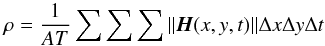 (18)where T is the number of time
samples in H and A is the area of the
telescope aperture.
(18)where T is the number of time
samples in H and A is the area of the
telescope aperture.
Figure 1a shows the measured densities for the 121 data sets of laboratory POAM experiments for the turbulence conditions shown in Table 1. The optical vortex density increases with both propagation distance and turbulence strength. Keep in mind that a smaller value of r0 corresponds to stronger turbulence strength.
Empirical observations have shown that optical vortices begin to appear in the beam at
 . This
is also the point at which the highest probability exists that a Laguerre-Gaussian beam
propagating through turbulence will undergo a ±
1 change of OAM state (Nairat &
Voelz 2014). Substituting this value into Eq. (16), using a single layer model for the turbulence profile and then
solving for the propagation distance gives the minimum propagation distance prior to the
onset of optical vortices as (Oesch et al. 2012),
. This
is also the point at which the highest probability exists that a Laguerre-Gaussian beam
propagating through turbulence will undergo a ±
1 change of OAM state (Nairat &
Voelz 2014). Substituting this value into Eq. (16), using a single layer model for the turbulence profile and then
solving for the propagation distance gives the minimum propagation distance prior to the
onset of optical vortices as (Oesch et al. 2012),
 (19)The remaining
strength dependence is accounted for by the normalization factor,
(19)The remaining
strength dependence is accounted for by the normalization factor,
 .
Figure 1b reflects the outcome of both of these
normalization steps. Nearly all of the measured densities appear to collapse onto a common
functional form. This suggests that the optical vortex density is a predictable parameter
of turbulence strength and distance. Combining these scaling terms and dimensional
analysis, the empirical function for density in laboratory data was found to be
.
Figure 1b reflects the outcome of both of these
normalization steps. Nearly all of the measured densities appear to collapse onto a common
functional form. This suggests that the optical vortex density is a predictable parameter
of turbulence strength and distance. Combining these scaling terms and dimensional
analysis, the empirical function for density in laboratory data was found to be
 (20)for a single turbulence
layer (Oesch et al. 2012), where the scaling
constant, Cρ =
Cr/Cs
= 2.91/[ (6.88)(0.5631) ] = 0.751.
(20)for a single turbulence
layer (Oesch et al. 2012), where the scaling
constant, Cρ =
Cr/Cs
= 2.91/[ (6.88)(0.5631) ] = 0.751.
Equation (20) can be thought of as describing the optical vortex density in the “non-saturated” regime. As can be seen from Fig. 1b, sufficient propagation distance and/or turbulence strength leads to deviations from the empirical function, i.e. “saturation”. The saturation effects begin at different densities for different turbulence strengths, all well below the maximum density that could be measured with this WFS, which is greater than 24 000 nov/ m2.
 |
Fig. 1 Optical vortex density from single phase wheel data for selected turbulence
strengths. For each curve, the turbulence strength, given by r0, is
held constant while the propagation distance is varied using the optical trombone.
a) Raw optical vortex density vs. propagation distance. b)
Optical vortex density normalized by |
3.3. Creation pair separation, δ
In contrast to the relatively simple estimation of the optical vortex density, there are a number of aspects that complicate estimating the pair separation, δ. The mod2π nature of the SRI phase includes 2π discontinuities in the measurement due to the wrapping. These wrapping discontinuities appear similar to branch cuts. Further, wrapping discontinuities can shift or mask branch cuts leading to confusion in identifying creation pairs. Noise can also create false circulations and branch cuts as well as obscure optical vortices. All of which further complicates the identification of creation pairs.
To overcome these issues, estimating the separation of creation pairs is a multi-step process (Oesch et al. 2012). Circulations are initially paired according to their connections through branch cuts in the phase. However, as the branch cuts can be influenced by local tilts two filtering steps are done to improve the confidence of the identified pairs. For each frame of WFS data, adding levels of constant phase to the mod2π phase, shifts the distribution of discontinuities in the mod2π phase that are not from POAM but the 2π wrapping of the measurement. Further the detections of pairs are tracked through multiple frames of the WFS. Together, scanning the piston and tracking through time leads to high confidence indications of the creation pairs in the WFS data.
Using this process, an estimate of the average pair separation, δ, was made for each of the configurations on Table 1. The result is plotted in Fig. 2 for the eleven turbulence strengths versus the scaled propagation distance as was done for density. Unlike density, separation doesn’t appear to have a strong dependence on the turbulence strength beyond that of z0.
 |
Fig. 2 Mean optical vortex separation plotted versus scaled propagation distance (z − z0). |
The functional form of the separation, shown in Fig. 2, appears to be proportional to  .
Fitting a function of this form to the curves gives,
.
Fitting a function of this form to the curves gives,  (21)where the scaling
constant, Cδ =
1/[CsCd] = 1/[(0.5631)(6.88)]=0.258 (Oesch et al. 2012). In
this relationship, the strength of the turbulence determines the minimum propagation
distance required for optical vortex pairs to form, but their separation beyond that point
is only a function of the wavelength and distance. Further there are no clear indications
of saturation effects in the separation curves shown in Fig. 2.
(21)where the scaling
constant, Cδ =
1/[CsCd] = 1/[(0.5631)(6.88)]=0.258 (Oesch et al. 2012). In
this relationship, the strength of the turbulence determines the minimum propagation
distance required for optical vortex pairs to form, but their separation beyond that point
is only a function of the wavelength and distance. Further there are no clear indications
of saturation effects in the separation curves shown in Fig. 2.
Interestingly further support for the form of the separation dependence comes from the
work of Tatarskii (1971). In discussing attempts to
determine a correlation radius for the intensity fluctuations of a horizontally
propagating beam, Tatarskii (1971) concluded that
his experiments to estimate a mean size of the inhomogeneities in the intensity would
always provide the same answer,  .
The mean size he was seeking can be thought of as the average distance between low
intensity regions. These are the regions in which branch points are found so their
separation should follow the same dependency identified by Tatarskii (1971).
.
The mean size he was seeking can be thought of as the average distance between low
intensity regions. These are the regions in which branch points are found so their
separation should follow the same dependency identified by Tatarskii (1971).
3.4. Projections of H
H represents three-dimensional POAM in the beam as mk in (x,y,t). Since turbulence varies smoothly, the optical vortex position, (xk(t),yk(t)), will also vary smoothly. As such, when optical vortices are present, H contains smooth tracks or “trails” (Oesch et al. 2013).
The temporal evolution of the optical vortices in the WFS data is captured in the
“projections” of the helicity spectrum (Oesch et al.
2010). The projections of H are defined as  (22)where
(N,M)
describes the sampling of the WFS, indexed by (i,j) over the x and y axes, respectively. The
projections compress the helicity information into two-dimensional representations of the
optical vortex motion relative to one of the WFS axes as x or y position vs. time;
xt or
yt
respectively.
(22)where
(N,M)
describes the sampling of the WFS, indexed by (i,j) over the x and y axes, respectively. The
projections compress the helicity information into two-dimensional representations of the
optical vortex motion relative to one of the WFS axes as x or y position vs. time;
xt or
yt
respectively.
Noise circulations in H can arise from camera noise, shot noise, bad camera frames, and subapertures with low signal-to-noise (SNR). Camera and shot noise lead to noise circulations appearing within H at random locations. Noise circulations from bad camera frames, appear as vertical lines in projxt(H) while noise circulations from subapertures with SNR issues produce horizontal lines in projxt(H) (Oesch et al. 2013), called fixed pattern noise.
Figure 3 shows an example of Eq. (22) applied to data from a bench-top experiment (Oesch et al. 2010). In the xt projection, the optical vortex trails form two sets with differing slopes, representing the two turbulence layer velocities of the ATS. A single optical vortex moving through the pupil in time with the moving turbulence layer forms a linear trail in the projection. The gray scale indicates the helicity of the circulations; m =−1 displayed in black and m = 1 in white.
 |
Fig. 3 Example of the projxt(H) from a set of laboratory data. The turbulence was generated by a two-layer atmospheric turbulence simulator. |
While Fig. 3 clearly shows many optical vortex trails they are really a series of trail segments. The turbulence generated by the ATS is effectively in frozen layers, so each generated optical vortex pair should move smoothly across the telescope aperture. All of the previously mentioned noise issues, combined with the discrete sampling of the detector leads to conditions where the trails appear discontinuous in the projection. In this example, many of the creation pairs are closely clustered together (i.e. a high density, ρ) and with small creation pair separations, δ. The high density can lead to multiple optical vortices within an elementary circulation canceling out (i.e. reducing the result of Eq. (17)). The small δ means the two points in a pair need to be found in separate elementary circulations in order to be detected. As the collection of optical vortices move across the WFS their individual positions within the geometry of the calculated elementary circulations changes. The result is the fragmented trails shown in Fig. 3.
While optical vortex trails in the projection of the helicity spectrum indicate the presence of POAM in the propagating beam, it is important to consider the full implication of what a trail signifies in terms of the field. A single trail is tracing the trajectory of the core of an optical vortex within the propagating field. Therefore, recalling Sect. 1, there is a Poynting vector winding its way around each trail along with a component of the electric field parallel to each trajectory. Additionally, the electric field components surrounding creation pairs diminish in magnitude with increased distance from the pair’s midpoint due to their opposite helicities. Therefore, the full set of trails shown in Fig. 3, only hints at the complexity of the underlying optical field.
3.5. Estimating the transverse velocity of a turbulence layer
As the laboratory turbulence is effectively a set of frozen layers, nov is not a
function of time. Therefore under such conditions an individual optical vortex pair will
travel uniformly through H. The motion of the optical
vortices demonstrated through the trails in the projections of H then conveys
information about the turbulence layer responsible for the formation of the optical vortex
pairs. By calculating 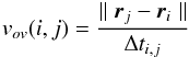 (23)where
ri = ⟨
xi(t),yi(t)
⟩ and rj = ⟨
xj(t),yj(t)
⟩, a set of instantaneous velocities can be determined for every two
optical vortices with like helicity at different points in time. Arranging the estimates
into bins of increasing velocity creates a velocity distribution, D(v). In
the velocity distribution, correlated measurements self-reinforce, and these lead to
spikes at the location of optical vortex velocities (Oesch
et al. 2010). These velocities are the transverse velocities of the turbulence
layers.
(23)where
ri = ⟨
xi(t),yi(t)
⟩ and rj = ⟨
xj(t),yj(t)
⟩, a set of instantaneous velocities can be determined for every two
optical vortices with like helicity at different points in time. Arranging the estimates
into bins of increasing velocity creates a velocity distribution, D(v). In
the velocity distribution, correlated measurements self-reinforce, and these lead to
spikes at the location of optical vortex velocities (Oesch
et al. 2010). These velocities are the transverse velocities of the turbulence
layers.
A laboratory demonstration (Oesch et al. 2010) measured these transverse velocities given by Eq. (23). This experiment featured five data sets each with two turbulence layers, low and high altitude, configured to return the same turbulence strength in all cases but where the phase screen velocities are varied. The turbulence layer velocities are described on Table 2.
Wind speeds for the velocity experiment.
The results of the experiment are plotted in Fig. 4. On the left are the projxt(H) while the velocity distribution, D(vx) is in the right column. The plots are arranged according to the configuration numbers given on Table 2. The characteristic correlation peaks in D(vx) are clearly visible in all cases.
The broad Gaussian-like background distribution centered at zero is due to cross-term velocities between trails from different optical vortices. Note that the vertical scale is changing to follow the decreasing peaks but that the distribution from the cross-terms remains constant.
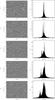 |
Fig. 4 Left column: xt projection of the helicity array. Right column: corresponding velocity distributions, D(vx). Note, the vertical lines seen in projections 1, 2, and 3 to the left are bad frames of wavefront sensor data; they have no significant effect on the peaks of D(vx), demonstrating the robustness of the technique. |
The velocities at the identified peaks from Fig. 4 are plotted in Fig. 5 where the magnitudes of the turbulence layer velocities and measured velocities are plotted against one another. For comparison, the exact case is indicated by the red line. In the laboratory with “thin”, frozen layers and very low noise the estimates of transverse velocity are nearly perfect.
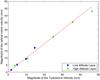 |
Fig. 5 Velocity magnitudes estimated versus theoretical. The correlation between the set velocity and measured velocity is remarkably high. Also note, there appears to be only four low altitude measurements because configurations #1 and #2 have the same low altitude turbulence layer velocity, and this causes the two measurements to overlay in the plots. |
4. Field experiments
A distributed volume atmosphere will naturally present some additional challenges not present in the idealized frozen layer turbulence of the laboratory. The distributed and evolving nature of the turbulence provides for the possibility of much more complicated spectrums, H. At the same time, the continuous and time-varying distribution of turbulence along the propagation path could provide a better environment for the formation of POAM than the thin and isolated laboratory simulations. Additionally, most field experiments use a Shack-Hartmann WFS rather than the SRI WFS used in the laboratory experiments.
4.1. The Shack-Hartmann WFS
The WFS of choice for astronomical adaptive optics applications is the Shack-Hartmann. The wave front is sampled at a plane conjugate to the telescope pupil using a lenslet array. This grid of small lenses (i.e. subapertures) creates a pattern of spots across a CCD camera in the image plane. As turbulence distorts the optical wave front, the positions of the spots change proportional to the local tilt within each subaperture. The position of each spot relative to the center of its associated subaperture gives a measurement of the local gradients of the phase, ∇φ(x,y).
Most field systems use much smaller numbers of subapertures than the 256 × 256 SRI in the laboratory experiments. However, the basis for the processing of circulations, Eq. (17), remains the same as does the construction of the helicity spectrum H, Sect. 2.1.4.
4.1.1. Optical vortex parameters (ρ, δ and v) in field experiments
As the construction of H remains unchanged, the calculation of the optical vortex density still follows Eq. (18).
The estimation of the creation pair separation, δ, on the other hand, is completely dependent on branch cuts in the mod2π phase. As the Shack-Hartmann returns only the gradients of the phase, estimation of δ is not possible by the method described in Sect. 3.3; further a method does not yet exist to do so.
Velocity distributions like those shown in Sect. 3.5 tend to be limited by the lower resolution of most Shack-Hartmann WFS. The projections of H, however, still provide a definitive means of identifying POAM in propagating optical fields through optical vortex trails.
4.1.2. Terrestrial example of proj(H)
As an example, field experiments over a three kilometer, near-horizontal propagation path using the Starfire Optical Range Turbulence Sensor (SORTS; Brennan & Mann 2010; Farrell et al. 2012) show turbulence-induced POAM (Oesch et al. 2013) in the projections of the helicity spectrums much like those found in the laboratory.
The SORTS instrument is a 40 cm Meade telescope fitted with a 32 × 32 Shack-Hartmann WFS which gathers gradient data similar to the 2011 SOR observations on the 3.5 m telescope.
An example xt projection from the SORTS instrument data is shown in Fig. 6 (Oesch et al. 2013). This data was collected at 8 KHz and so the 2000 frame set represents 0.25 s of atmospheric data. The formation of trails in distributed volume turbulence requires that the rate of change of the turbulence is slow compared to the frame rate of the optical system.
The x-axis of the SORTS instrument was horizontal while the y-axis was vertical. In this experiment, the wind was predominately along the x-axis, so only the xt projection is shown in Fig. 6. The projection shows a series of trails with consistent slope, indicating a predominately-constant, horizontal wind speed associated with the optical vortex producing turbulence.
 |
Fig. 6 Terrestrial experiment demonstrating turbulence-induced, optical vortex trails using the projection of the helicity spectrum, H onto the xt plane. |
This projection shows the same optical vortex behavior as the laboratory results using one or two phase screens, see Figs. 3 and 4, demonstrating that the laboratory characterization of turbulence-induced POAM can be extended to real-world turbulence conditions (Oesch et al. 2010, 2012, 2013).
5. Turbulence-induced POAM in Astronomy
The application of the helicity spectrum analysis to stellar observations allows astronomers to use POAM as a novel probe of astronomical systems. Sanchez et al. (2013) showed that astronomical TAMA are capable of inducing POAM in starlight.
5.1. Astronomical TAMA and EM fields
The mechanism for the formation of POAM in astronomical TAMA is the same as for turbulence within the Earth’s atmosphere, though perhaps at a much slower rate (Sanchez et al. 2013). For example the densities in the Orion nebula are much lower, 103 − 109 cm-3 (Nissen et al. 2007; López-Sepulcreand et al. 2013), than those for the Earth’s atmosphere, 1016 cm-3.
Equation (3) still describes the mechanic through which light encountering the nebula acquires POAM. The spatial scale of fluctuations in n(r,t) is much larger and therefore the rate of POAM formation much slower than atmospherically-induced POAM. However, the full nature of turbulence-induced POAM is still unknown at AU or pc sizes. The scales involved when dealing with astronomical sources of POAM have an impact on the measurements in a number of ways.
5.2. Measuring astronomical POAM
To measure POAM from any astronomical source requires that the intervening TAMA is resolved by the optical system (Elias 2008). Note that this is a measurement issue which has no bearing on the intrinsic POAM of the propagating wave. The angular resolution of a 3.5 m telescope is 39.5 mas at a wavelength of 550 nm. The disk surrounding 49 Ceti has an angular extent of approximately 29.5 arcsec. The Trapezium cluster covers nearly 22 arcmin of the much larger Orion nebula which covers approximately 1°. Therefore, the known TAMA associated with the two stars, 49 Ceti and HR 1895, were clearly resolved for these observations.
5.3. Astronomical optical vortex density
Habibi et al. (2011) investigated the prospect of locating interstellar gas through scintillation induced on propagating light. Optical scintillation and the formation of POAM are closely related. He simulated light from distant stars propagating through clouds of interstellar gas to an observer. Based on the Kolmogorov theory of optical turbulence, the gas was approximated as “thin” layers in the same way the ASALT laboratory POAM experiments were conducted, Sect. 3.
Habibi et al. (2011) scaled the turbulence
strength as the diffusion radius, Rdiff, which is proportional to the
coherence length, r0, for atmospheric turbulence;
r0 =
3.18Rdiff (Narayan 1992). For an astronomical cloud then, ![Mathematical equation: \begin{equation} \label{eq: Rdiff} r_0 = 836.3 \ {\rm Km} \left[ \frac{\lambda}{1 ~\mu\rm m} \right]^{\frac{6}{5}} \left[ \frac{L_z}{10\rm ~ AU} \right]^{-\frac{1}{5}} \left[ \frac{\sigma_{3n}}{10^9~ \rm cm^{-3}} \right]^{-\frac{6}{5}}, \end{equation}](/articles/aa/full_html/2014/07/aa23140-13/aa23140-13-eq150.png) (24)where Lz is the scale size of
fractal structures within the cloud and σ3n is the dispersion
of the volume number density which is limited by the number density of the medium (Habibi et al. 2011). His analysis lead to estimated
values of Rdiff =
17 Km for Lz = 30 AU size
“clumpuscules” within a much larger interstellar cloud having a mean density of
1010
cm-3 at
λ = 1.25
μm which demonstrates sufficient strength to cause
scintillation. Light propagating through such turbulence would begin to form POAM after
z0 = 0.05
pc using the experimental laboratory results in Sect. 3.
(24)where Lz is the scale size of
fractal structures within the cloud and σ3n is the dispersion
of the volume number density which is limited by the number density of the medium (Habibi et al. 2011). His analysis lead to estimated
values of Rdiff =
17 Km for Lz = 30 AU size
“clumpuscules” within a much larger interstellar cloud having a mean density of
1010
cm-3 at
λ = 1.25
μm which demonstrates sufficient strength to cause
scintillation. Light propagating through such turbulence would begin to form POAM after
z0 = 0.05
pc using the experimental laboratory results in Sect. 3.
Applying Habibi’s analysis to the Orion nebula, Orion can be thought of as a collection of dense molecular clouds, with sizes on the order of 2 pc (López-Sepulcreand et al. 2013). Using this size as Lz in Eq. (24) along with the density of 109 cm-3 gives r0 ~ 77 Km at 0.55 μm.
Continuing with the assumptions used by Habibi et al. (2013), optimistically, the empirically derived laboratory expressions, Sect. 3, can frame what might be detectable from such a TAMA.
Empirically then, a turbulence layer at approximately 420 pc with r0 ~ 77 Km would begin to generate POAM no sooner than z0 ~ 0.1 pc. This is the minimum distance because it is based on the maximum density for the Orion molecular cloud, 109 cm-3. For this model, Eq. (20), estimates a maximum density on the order of ρ ≤ 4.2 nov/ m2.
Further, setting the minimum distance for branch points to form from a turbulence layer, z0, equal to the distance to Orion gives the lowest density that can form POAM at Earth as 108 cm-3. Therefore under these approximations only the densest portions of the molecular cloud are likely to contribute to POAM measurements. However, it is known from the laboratory experiments that multiple turbulence layers create more optical vortices than the sum of the individual layers alone (Oesch et al. 2010). Therefore, the far more complicated structure of the Orion Molecular Cloud will likely generate POAM through the interaction of multiple layers of lower density.
5.4. Transverse velocity
In laboratory experiments and wave optical simulation, the slopes of the optical vortex trails provide estimates of the transverse motion of the intervening turbulence (Oesch et al. 2012). Applied to astronomical TAMA, this benefit of the POAM measurement offers astronomers a novel means of estimating motion perpendicular to the line of sight; something that is not available in most observations.
The estimate of the transverse velocity, vt, is given by the ratio of the number
of subapertures, nsub, to the number of frames,
nf, spanned by an optical vortex trail
times the product of the subaperture diameter, d, and the frame rate of the system,
F,
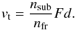 (25)For SOR’s
3.5 m, 24 × 24 Shack-Hartmann WFS, detections of an
optical vortex at a subaperture per frame (nsub/nfr =
1) corresponds to a transverse velocity of Fd = 292 m /
s. Speeds higher than a subaperture per frame are increasingly less
likely to be distinguishable as trails in the presence of noise and other optical
vortices. Slower speeds offer the possibility of multiple detections of an optical vortex
within the same subaperture, which is beneficial in opposing some of the issues in the
formation of an identifiable trail. This implies an upper limit on the transverse velocity
measurable using the SOR 3.5 m
telescope adaptive optics with this approach on the order of 300 m/s.
(25)For SOR’s
3.5 m, 24 × 24 Shack-Hartmann WFS, detections of an
optical vortex at a subaperture per frame (nsub/nfr =
1) corresponds to a transverse velocity of Fd = 292 m /
s. Speeds higher than a subaperture per frame are increasingly less
likely to be distinguishable as trails in the presence of noise and other optical
vortices. Slower speeds offer the possibility of multiple detections of an optical vortex
within the same subaperture, which is beneficial in opposing some of the issues in the
formation of an identifiable trail. This implies an upper limit on the transverse velocity
measurable using the SOR 3.5 m
telescope adaptive optics with this approach on the order of 300 m/s.
Above this upper limit, the number of possible repeated detections of an individual optical vortex decreases. For the 3.5 m AO system at any speed, nsub ≤ 23, typically less due to the secondary obscuration. Reductions in nsub due to high speeds leads to a few widely spaced detections, not a clear trail. Instead the individual optical vortex detections appear isolated and random.
As an example of observatory-TAMA relative motion, Castañeda (1988) measured relative gas velocities in the Orion nebula, on the order of 10 Km s-1. Even at 3 Km s-1, near the lowest measured velocity, the equivalent of 10 subapertures per frame, at most three circulations are recorded for each optical vortex on the SOR AO WFS. Individual trails are not identifiable at that rate, especially in the presence of other optical vortices and noise. It is likely that any optical vortices formed from the Orion Nebula in the 2011 SOR observations will appear like random noise circulations.
6. POAM in the 2011 SOR observations
The 2011 SOR observations were conducted using the Air Force Research Laboratory, Directed Energy Directorate’s 3.5 m telescope located at the SOR on Kirtland AFB, NM. The data was collected using the natural guide star adaptive optics (AO) system which features a 24 × 24 Shack-Hartmann WFS run in open loop with a 2 KHz frame rate in the wavelength range of 450−650 nm. The system collected wave front gradient data in 11 and 21 s captures.
6.1. POAM estimation through η
In the initial analysis of the 2011 SOR observations, the presence of POAM was estimated
using the conversion efficiency; a first order approximation of the amount of the light
that has been transformed from an m = 0 to any m ≠ 0 state. The
calculation depends on the distribution of the gradients between the two associated
Hilbert spaces for the rotational and non-rotational (least-mean-square) phase components
through the summation of the norms of their respective gradients (Sanchez et al. 2013);
![Mathematical equation: \begin{eqnarray} \left[ \left[ \mathcal{G}_{\rm lms} \right] \right] & = &\sum_{i\,=\,1}^N \sum_{j\,=\,1}^M \| \nabla \phi_{\rm lms} \| \nonumber \\ \left[ \left[ \mathcal{G}_{\rm rot} \right] \right] & = &\sum_{i\,=\,1}^N \sum_{j\,=\,1}^M \| \nabla \phi_{\rm rot} \|, \end{eqnarray}](/articles/aa/full_html/2014/07/aa23140-13/aa23140-13-eq185.png) (26)where
N ×
M defines the number of subapertures in the lenslet
array. The conversion efficiency is constructed from the ratio of these sums as
(26)where
N ×
M defines the number of subapertures in the lenslet
array. The conversion efficiency is constructed from the ratio of these sums as
![Mathematical equation: \begin{equation} \eta = \frac{ \left[ \left[ \mathcal{G}_{\rm rot} \right] \right] }{ \left[ \left[ \mathcal{G}_{\rm rot} \right] \right] + \left[ \left[ \mathcal{G}_{\rm lms} \right] \right] }\cdot \end{equation}](/articles/aa/full_html/2014/07/aa23140-13/aa23140-13-eq187.png) (27)A main advantage of
η for
estimation of the POAM signal is that the ratio eliminates multiplicative scaling terms in
the measurement.
(27)A main advantage of
η for
estimation of the POAM signal is that the ratio eliminates multiplicative scaling terms in
the measurement.
Table 3 shows the original results of the 2011 SOR observations from Sanchez et al. (2013) by star name and observation time. The 2011 conversion efficiencies are provided along with the relative signal strengths as the number of standard deviations above the noise floor, Nσ. Recall that in the original estimation of the signal strengths, the noise floor was set very conservatively at ηfloor = 0.04.
2011 SOR observations.
6.2. POAM estimation through ρ
For each of the ten observations conducted in 2011, the data was reprocessed to construct a helicity spectrum, H. That processing also provides a measurement of the density of the optical vortices, ρ. Table 4 shows the estimated densities for the 10 observations conducted in 2011 at the SOR. These will be discussed in more detail along with each star in the next section.
2011 SOR observation comparing estimates of η with the measured optical vortex density, ρ.
6.3. POAM estimation through proj(H)
In this section, each of the five stars are evaluated in turn and the projections of the helicity spectra are examined briefly with further discussion in Sect. 7.
6.3.1. 49 Ceti
49 Ceti is an A1 V star at a distance of approximately 61 pc (ESA 1997) with a well studied debris disk of gas and dust extending out to 900 AU (Wahhaj et al. 2007; Hughes et al. 2008). In the original analysis, observations of 49 Ceti were indicated to have a 2σ POAM signal (Sanchez et al. 2013).
49 Ceti shows strong optical vortex trails in both the xt and yt projections of H, see Fig. 7. The clear optical vortex trails in the projections confirm the presence of POAM in the electromagnetic field. Note that, unlike the terrestrial field tests and laboratory experiments, both the xt and yt projections are included as there was no preferential alignment between the Shack-Hartmann WFS axis and the motion of the turbulence.
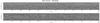 |
Fig. 7 Projections of H onto the xt and yt planes for the observation of 49 Ceti. |
Additionally there are many circulations captured in H that are not linked to the optical vortex trails in the projections.
6.3.2. HR 1529
HR 1529 is a K2 III star at approximately 72 pc (ESA 1997) in the constellation Aurigae. The original estimates set this observation at a 3σ POAM signal (Sanchez et al. 2013).
The projections from each observation contain optical vortex trails (see Fig. 8). The optical vortex trails from the Nov. 1st observations are better defined than those in the Oct. 31st even though both have comparable densities; 2.8 and 2.9 nov/ m2 respectively. The projections from Nov. 1st suggest that the optical vortex motion was largely favoring the x-axis while the Oct. 31st appears fairly balanced between x and y directions. Both sets of observations show fixed pattern noise.
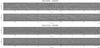 |
Fig. 8 Projections of H onto the xt and yt planes for the two observations of HR 1529. |
To improve the visibility of the optical vortex trails in high density cases, such as these, partial projections of H, ∂proj(H) (see Appendix A), create a clearer projection of the optical vortex trails. Figure 9 shows ∂proj(H) for HR 1529.
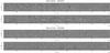 |
Fig. 9 Partial projections H onto the xt and the yt planes for the two observations of HR 1529. |
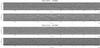 |
Fig. 10 Projections of H onto the xt and yt planes for the two observations of HR 1577. |
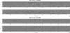 |
Fig. 11 Partial projections H onto the xt and the yt planes for the two observations of HR 1577. |
The partial projections also provide a better view of the circulations that are not associated with the dominant optical vortex trails or fixed pattern noise.
6.3.3. HR 1577
ι Aurigae (HR 1577) is a K3 II star at approximately 157 pc (ESA 1997). It is thought to be evolving from a main sequence B star towards the red giant branch (Harper 1992). Interestingly, both Silva et al. (2011) and Harper (1992) studied HR 1577 for evidence of turbulence. However, they were looking at turbulence in the photospheres of G and K stars whereas Sanchez et al. (2013) was looking for TAMA between the Earth and the candidate stars. The original analysis concluded that any POAM signal was below the noise floor of the detector.
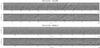 |
Fig. 12 Projections of H onto the xt and yt planes for the two observations of HR 1784. |
The observations of HR 1577 contain optical vortex trails in the projections of the helicity spectrum, H (see Fig. 10). The appearance of optical vortex trails clearly means that POAM was present in these observations contrary to the original conclusions (η = 0.04 and 0.03 respectively). However, the density estimates for these two data sets are the lowest of the ten observations at 1.6 and 1.2 nov/ m2. These low densities are evident in the partial projections of H shown in Fig. 11.
6.3.4. HR 1784
HR 1784 is a G8 III star at approximately 53 pc (ESA 1997) which is also a member of the recent 172 star photospheric study of G and K type stars (Silva et al. 2011). As with the observations of HR 1577, the original analysis of HR 1784 concluded that any POAM signal was below the noise floor of the detector.
However, Fig. 12 shows that there are once again well defined and tightly constrained optical vortex trails in these observations. The optical vortex densities (3.3 and 3.1 nov/m2) of these observations were comparable to those of HR 1529 which, based on its η estimate, was originally identified as a 3σ POAM signal.
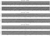 |
Fig. 13 Projections of H onto the xt and yt planes for the three observations of HR 1895. |
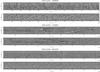 |
Fig. 14 Partial projections H onto the xt and the yt planes for the three observations of HR 1895. |
6.3.5. HR 1895
θ Orionis C (HR 1895) is an O6 star at approximately 490 pc (ESA 1997) in the center of the Trapezium cluster within the Orion nebula. It is a variable X-ray source thought to be driven by a strong magnetic field with a period of approximately 15 days (Gagné et al. 1997). The original analysis showed two levels of signal with one observation well above the noise floor and the other two at or below it. The two different signal levels were the instigator for the reanalysis done in this paper.
The projections of the helicity spectrums from the three nights of observations clearly show signs of optical vortex trails in all three. The estimated densities; 8.4, 3.4 and 2.9 nov/ m2, followed the trend of the estimated conversion efficiencies; 0.17, 0.05 and 0.04 respectively. Also, all three of the observations contain a POAM signal. The partial projections of the HR 1895 data are shown in Fig. 14.
6.4. Summary of results
While the original analysis of the 2011 SOR observations demonstrated the first detections of POAM signals from starlight; that analysis, only indicated a signal from 3 of the 5 candidate stars. This reanalysis shows that all ten of the observations contain optical vortex trails, confirming the presence of POAM in all cases.
6.4.1. Noise in the astronomical projections
Noise in its various forms appears in all of the projections of the 2011 SOR observations. Apparently random circulations appear throughout the 2011 SOR observations; see for instance, those of HR 1577 in Fig. 11. This type of noise establishes ηfloor.
An excellent example of fixed pattern noise appears in the HR 1895, Nov. 4th observations as two lines running down the center of the projection, see Fig. 14. The location of these fixed circulations suggests a poorly illuminated subaperture bordering the secondary obscuration.
The best example of noise interfering with detections of an optical vortex appears as a broken optical vortex trail in the ∂projxt(H) for the Oct. 31st observation of HR 1577 between frames 7500−10 000 in Fig. 11.
7. Discussion
Here the optical vortex trails identified in the 2011 SOR observations are discussed. First, as indications of the POAM content of the astronomical observations. Then the trails are considered as a tool for establishing a better limit on the noise floor in the POAM estimate, η, on the 3.5 m AO system. Lastly, instrumental considerations for a future astronomical POAM detector are considered.
7.1. POAM in starlight
Sanchez et al. (2013) demonstrated that any TAMA has the potential to induce POAM in propagating waves. In the original analysis the conversion efficiency was an attempt to gauge to what degree the propagating electromagnetic field had been impacted by an intervening TAMA. This work however has focused on tracking the motion of individual optical vortices within the WFS data. The well-defined optical vortex trails found in the 2011 observations are definitive indicators of POAM within the propagating optical wave.
Beginning with 49 Ceti and HR 1529, the method of projections confirm the earlier conclusion that there were indeed POAM signals in these observations. Figure 9 shows the partial projections for the observations of HR 1529. The partial projections of the Nov. 1st observation show well-constrained trails oriented strongly along a common slope throughout the helicity spectrum in both the x and y directions. While those of the Oct. 31st observation reveal either a broader range of slopes or multiple sets of slopes implying a more complicated and/or an evolving structure to the POAM generating turbulence.
The observations of HR 1577 and HR 1784 were both originally relegated to noise. The method of projections shows well-defined optical vortex trails, clearly demonstrating the presence of POAM in each of these data sets. Even the relative low optical vortex densities of HR 1577 show clean trails.
The observations of HR 1895 are unique amongst the sets collected in the 2011 SOR experiment. The first night of data taken on Nov. 1st had the highest value of η = 0.17 presented in the original research (Sanchez et al. 2013), while the two later nights collected POAM signals near the original estimate of the noise floor, 0.05 and 0.04. The measured densities and η show similar results with the highest η estimate corresponding to the highest measured density, ρ = 8.4 nov/m2, while the other two sets had more modest densities of 3.4 and 2.9 nov/ m2 respectively.
The projections of the helicity spectrum for each of these data sets are shown in Fig. 13. Optical vortex trails are clearly visible in the projections of the Nov. 1st and 4th data.
The projection of the Nov. 3rd data in Fig. 13 appears quite different from any of the other data sets. At first glance it has similarities with the Oct. 31st observations of HR 1529 where there appears to be a range of optical vortex slopes. Looking closely at the partial projection of the Nov. 3rd data observations, Fig. 14, also reveals some nearly horizontal trails; i.e. slow moving optical vortices.
7.2. Reevaluation of η
In the original analysis of the 2011 SOR observations, Sanchez et al. (2013) developed a metric for estimating the signal that is invariant to multiplicative scaling errors and isn’t limited by the low number and large diameter of the subapertures of the 3.5 m telescope WFS. This metric proved to be a simple and direct method of estimating the POAM content of the electromagnetic field. At that time, a good means of estimating the noise floor of the system was not available.
Considering the results of Sect. 6.3 a better estimate of the noise floor for the 3.5 m AO system can now be made. Identifying an upper limit begins with the original η estimations found in Table 3, specifically concentrating on the lowest estimate of η (HR 1577 at η = 0.03 ± 0.004). Comparison of the full and partial projections of the HR 1577 observation of Nov. 1st (Figs. 10 and 11) shows that the corresponding optical vortex density, ρ = 1.2 nov/ m2 (the lowest of the measured values), is still above the noise limits of the system. The partial projections shown in Sect. 6.3 reflect an effective reduction to approximately 1/3rd of the full useable system aperture. That these partial projections still indicate trails, suggests that even at 1/3rd of the lowest measured density, the system would still be operating above the noise floor. Therefore, reducing the number of optical vortices contributing to the gradient sums suggests ηfloor ≤ 0.01.
Returning to the estimates of the signal levels, Nσ is recalculated based on this new ηfloor. Table 5 compares the estimated POAM signals for each of the 2011 SOR observations in terms of the original noise floor estimates done in 2012 along side the current upper bound of the noise (2013). These new values clearly reflect the same results obtained from the method of projections; that all of the 2011 observations possessed strong POAM signals.
Comparison of the results of 2011 SOR observation estimates of the POAM signal strength, Nσ, from the original estimates (2012) and the results of calculations based on the new upper bound for POAM signals done here (2013).
7.3. Astronomical TAMA
The majority of the trails visible in Figs. 7−14 possess slopes on the order of 10 m/s, suggesting a terrestrial origin. Since independent measurements of the Earth’s atmosphere as an intervening TAMA were unavailable, analysis of these trails is left to a future paper.
Discounting the optical vortex trails of terrestrial origin, a large number of circulations that are not fixed pattern noise remain above the noise floor; the Oct. 31st observations for HR 1529 (see Fig. 8) for instance. A portion of these circulations may be detections of optical vortices with velocities too high to form trails with this instrument. The upper limit of 300 m /s is greater than all terrestrial wind speeds. Optical vortices with velocities greater than this limit would appear random and disconnected, not as trails. Therefore, optical vortex detections in this group may be associated with astronomical TAMA along the line of sight to the observed star. The density distributions, temporal evolution and relative motions of source TAMA like the Orion nebula or the circumstellar disk of 49 Ceti for POAM creation are not yet fully understood. The work of Sanchez et al. (2013) demonstrates that such systems will produce POAM. However, it is likely that any optical vortex detections from these systems belong to the circulations not associated with these trails. A dedicated POAM WFS will be necessary to examine this possibility in future experiments.
7.4. Future detector
Design of a future detector which uses the projections of the helicity spectrum must consider the transverse velocity. For instance, two orders of magnitude separate the velocity limit of the SOR AO system from capturing trails on the order of the Earth’s orbital velocity. However, increases to the aperture size, the total number of subapertures and/or decreases to the subaperture diameters offer other means of achieving the same goal.
8. Summary
This work confirms that turbulence-induced POAM has been successfully observed in every instance of ASALT laboratory, simulation and field experiments including the 2011 Starfire Optical Range astronomical observations (Sanchez et al. 2013). This paper’s reevaluation of the 2011 SOR observations validates the assertion that the creation of POAM is a customary byproduct of astronomical light propagating through turbulence. Finally this analysis identifies that there are significant numbers of circulations that are not associated with terrestrial optical vortex trails.
References
- Allen, L., Beijersbergen, M. W., Spreeuw, R. J. C., & Woerdman, J. P. 1992, Phys. Rev. A, 45, 8185 [NASA ADS] [CrossRef] [PubMed] [Google Scholar]
- Berkhout, G. C., Lavery, M. P. J., Courtial, J., Beijersbergen, M. W., & Padgett, M. J. 2010, Frontiers in Optics OSA, FMB5 [Google Scholar]
- Berkhout, G. C. G., & Beijersbergen, M. W. 2010, Phys. Rev. Lett., 101, 0801 [Google Scholar]
- Brennan, T. J., & Mann, D. C. 2010, Proc. SPIE, 7816, 781602 [CrossRef] [Google Scholar]
- Castañeda, H. O. 1988, ApJSS, 67, 93 [NASA ADS] [CrossRef] [Google Scholar]
- Chen, M., Mazilu, M., Arita, Y., Wright, E. M., & Dholakia, K. 2013, Opt. Lett., 38, 4919 [NASA ADS] [CrossRef] [Google Scholar]
- Cristi, R., & Axtell, T. W. 2013, J. Opt. Soc. Am. A, 30, 2225 [NASA ADS] [CrossRef] [Google Scholar]
- Elias, II, N. M. 2008, A&A, 492, 883 [NASA ADS] [CrossRef] [EDP Sciences] [Google Scholar]
- ESA. 1997, The Hipparcos and Tycho Catalogues, ESA SP, 1200 [Google Scholar]
- Farrell, T. C., Sanchez, D. J., Smith, J. C., et al. 2012, in Unconventional Imaging and Wavefront Sensing VIII, eds. J. J. Dolne, T. J. Karr, V. L. Gamiz, & D. C. Dayton, 8520 (SPIE Press), 85200H [Google Scholar]
- Fried, D. L. 1965, J. Opt. Soc. Am., 55, 1427 [NASA ADS] [CrossRef] [Google Scholar]
- Fried, D. L. 1998, J. Opt. Soc. Am. A, 15, 2759 [NASA ADS] [CrossRef] [Google Scholar]
- Gagné, M., Jean-Pierre, Caillault,Stauffer, J. R., & Linsky, J. L. 1997, ApJ, 478, L87 [NASA ADS] [CrossRef] [Google Scholar]
- Gibson, G., Courtial, J., Padgett, M. J., et al. 2004, Opt. Express, 12, 5448 [Google Scholar]
- Gruneisen, M. T., Miller, W. A., Dymale, R. C., & Sweiti, A. M. 2008, Appl. Opt., 47, A32 [NASA ADS] [CrossRef] [Google Scholar]
- Habibi, F., Moniez, M., Ansari, R., & Rahvar, S. 2011, A&A, 525, A108 [NASA ADS] [CrossRef] [EDP Sciences] [Google Scholar]
- Habibi, F., Moniez, M., Ansari, R., & Rahvar, S. 2013, A&A, 552, A93 [NASA ADS] [CrossRef] [EDP Sciences] [Google Scholar]
- Harper, G. M. 1992, MNRAS, 256, 37 [NASA ADS] [CrossRef] [Google Scholar]
- Harwit, M. 2003, ApJ, 597, 1266 [NASA ADS] [CrossRef] [Google Scholar]
- Hughes, A. M., Wilner, D. J., Kamp, I., & Hogerheijde, M. R. 2008, ApJ, 681, 626 [NASA ADS] [CrossRef] [Google Scholar]
- Jackson, J. D. 1975, Classical Electrodynamics, 2nd edn. (New York, USA: John Wiley & Sons) [Google Scholar]
- Kim, D. J., Kim, J. W., & Clarkson, W. A. 2013, Opt. Express, 21, 29449 [NASA ADS] [CrossRef] [Google Scholar]
- Kolmogoroff, A. N. 1941, Comptes Rendus de l’Académie des Sciences de l’URSS, 31, 538 [Google Scholar]
- Lavery, M. P. J., Berkhout, G. C. G., Courtial, J., & Padgett, M. J. 2011a, J. Opt., 13, 4006 [NASA ADS] [CrossRef] [Google Scholar]
- Lavery, M. P. J., Robertson, D. J., Courtial, J., et al. 2011b, in Frontiers in Optics 2011/Laser Science XXVII, OSA Technical Digest (Optical Society of America) [Google Scholar]
- López-Sepulcreand, A., Kama, M., Ceccarelli, C., et al. 2013, A&A, 549, A114 [NASA ADS] [CrossRef] [EDP Sciences] [Google Scholar]
- Mantravadi, S. V., Rhoadarmer, T. A., & Glas, R. S. 2004, in Advanced Wavefront Control: Methods, Devices, and Applications II, eds. M. K. Giles, J. D. Gonglewshi, & R. A. Carerras, Proc. SPIE, 5553, 290 [Google Scholar]
- Nairat, M., & Voelz, D. 2014, Optic. Lett., 39, 1838 [NASA ADS] [CrossRef] [Google Scholar]
- Narayan, R. 1992, Phil. Trans. Roy. Soc. London Ser., A, 341, 151 [Google Scholar]
- Nissen, H. D., Gustafsson, M., Lemaire, J. L., et al. 2007, A&A, 466, 949 [NASA ADS] [CrossRef] [EDP Sciences] [Google Scholar]
- Oemrawsingh, S. S. R., van Houweilingen, J. A. W., Eliel, E. R., et al. 2004, Appl. Opt., 43, 688 [NASA ADS] [CrossRef] [PubMed] [Google Scholar]
- Oesch, D. W., & Sanchez, D. J. 2012, Opt. Express, 20, 12292 [NASA ADS] [CrossRef] [Google Scholar]
- Oesch, D. W., Sanchez, D. J., & Matson, C. L. 2010, Opt. Express, 18, 22377 [NASA ADS] [CrossRef] [Google Scholar]
- Oesch, D. W., Tewksbury-Christle, C. M., Sanchez, D. J., & Kelly, P. R. 2012, Opt. Eng., 51, 6001 [NASA ADS] [CrossRef] [Google Scholar]
- Oesch, D. W., Sanchez, D. J., Gallegos, A. L., et al. 2013, Opt. Express, 21, 5440 [NASA ADS] [CrossRef] [Google Scholar]
- Rhoadarmer, T. A. 2004, in Advanced Wavefront Control: Methods, Devices, and Applications II, eds. M. K. Giles, J. D. Gonglewshi, & R. A. Carerras, Proc. of the SPIE, 5553, 112 [Google Scholar]
- Roux, F. 2013, Opt. Lett., 38, 3895 [NASA ADS] [CrossRef] [Google Scholar]
- Ruane, G. J., & Swatzlander, Jr. G. A., 2013, Appl. Opt., 52, 171 [NASA ADS] [CrossRef] [Google Scholar]
- Sanchez, D. J., & Oesch, D. W. 2009, in Advanced Wavefront Control: Methods, Devices, and Applications VII, eds. R. A. Carerras, T. A. Rhoadarmer, & D. C. Dayton, Proc. of the SPIE, 7466, 0501 [Google Scholar]
- Sanchez, D. J., & Oesch, D. W. 2011a, Opt. Express, 19, 25388 [Google Scholar]
- Sanchez, D. J., & Oesch, D. W. 2011b, Opt. Express, 19, 24596 [NASA ADS] [CrossRef] [Google Scholar]
- Sanchez, D. J., Oesch, D. W., & Reynolds, O. R. 2013, A&A, 556, A130 [NASA ADS] [CrossRef] [EDP Sciences] [Google Scholar]
- Sasiela, R. J. 2007, Electromagnetic Wave Propagation in Turbulence: Evaluation and Application of Mellin Transforms, 2nd edn. (Bellingham: SPIE Press) [Google Scholar]
- Shalaev, M. I., Kudyshev, Z. A., & Litchinitser, H. M. 2013, Opt. Lett., 21, 4288 [NASA ADS] [CrossRef] [Google Scholar]
- Silva, R. D., Milone, A. C., & Reddy, B. E. 2011, A&A, 526, A71 [NASA ADS] [CrossRef] [EDP Sciences] [Google Scholar]
- Sponselli, A., & Lavery, M. P. 2013, Imaging and Applied Optics OSA, PTu3F [Google Scholar]
- Sun, J., Zeng, J., & Litchinister, N. M. 2013, Opt. Express, 21, 14975 [Google Scholar]
- Tamburini, F., Mari, E., Sponselli, A., et al. 2012, New J. Phys., 14, 033001 [NASA ADS] [CrossRef] [Google Scholar]
- Tatarskii, V. I. 1971, The Effects Of Turbulent Atmosphere On Wave Propagation (Jerusalem: Israel Program for Scientific Translations Ltd.) [Google Scholar]
- Wahhaj, Z., Koerner, D. W., & Sargent, A. I. 2007, ApJ, 661, 368 [NASA ADS] [CrossRef] [Google Scholar]
- Yao, A. M., & Padgett, M. J. 2011, Adv. Opt. Photon., 3, 161 [CrossRef] [Google Scholar]
Appendix A: Partial projections
Projections of H are a two-dimensional image of the motion of the optical vortices in the WFS measurement. The use of the projection is limited by the density of the circulations present in any measurement. Low signal to noise or high POAM signals (large concentrations of optical vortex trails) can obscure the appearance of the trails in the full projection.
In the case of high optical vortex density with no preferential alignment between the WFS
and the turbulence, as in the case of the 2011 SOR observations, it was found that using
the sum of three cross-sections of H to create a partial projection
i.e. 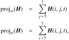 (A.1)can
clarify the appearance of the optical trails by reducing the concentration of the
circulations in the projection. The indices of 5−7 were chosen to avoid the obscuration of the 3.5 m telescope’s
secondary mirror within the WFS data.
(A.1)can
clarify the appearance of the optical trails by reducing the concentration of the
circulations in the projection. The indices of 5−7 were chosen to avoid the obscuration of the 3.5 m telescope’s
secondary mirror within the WFS data.
All Tables
Turbulence conditions used for measurement of optical vortex density and separation, based on a 1.5 m aperture.
2011 SOR observation comparing estimates of η with the measured optical vortex density, ρ.
Comparison of the results of 2011 SOR observation estimates of the POAM signal strength, Nσ, from the original estimates (2012) and the results of calculations based on the new upper bound for POAM signals done here (2013).
All Figures
|
Fig. 1 Optical vortex density from single phase wheel data for selected turbulence
strengths. For each curve, the turbulence strength, given by r0, is
held constant while the propagation distance is varied using the optical trombone.
a) Raw optical vortex density vs. propagation distance. b)
Optical vortex density normalized by |
| In the text | |
|
Fig. 2 Mean optical vortex separation plotted versus scaled propagation distance (z − z0). |
| In the text | |
|
Fig. 3 Example of the projxt(H) from a set of laboratory data. The turbulence was generated by a two-layer atmospheric turbulence simulator. |
| In the text | |
|
Fig. 4 Left column: xt projection of the helicity array. Right column: corresponding velocity distributions, D(vx). Note, the vertical lines seen in projections 1, 2, and 3 to the left are bad frames of wavefront sensor data; they have no significant effect on the peaks of D(vx), demonstrating the robustness of the technique. |
| In the text | |
|
Fig. 5 Velocity magnitudes estimated versus theoretical. The correlation between the set velocity and measured velocity is remarkably high. Also note, there appears to be only four low altitude measurements because configurations #1 and #2 have the same low altitude turbulence layer velocity, and this causes the two measurements to overlay in the plots. |
| In the text | |
|
Fig. 6 Terrestrial experiment demonstrating turbulence-induced, optical vortex trails using the projection of the helicity spectrum, H onto the xt plane. |
| In the text | |
|
Fig. 7 Projections of H onto the xt and yt planes for the observation of 49 Ceti. |
| In the text | |
|
Fig. 8 Projections of H onto the xt and yt planes for the two observations of HR 1529. |
| In the text | |
|
Fig. 9 Partial projections H onto the xt and the yt planes for the two observations of HR 1529. |
| In the text | |
|
Fig. 10 Projections of H onto the xt and yt planes for the two observations of HR 1577. |
| In the text | |
|
Fig. 11 Partial projections H onto the xt and the yt planes for the two observations of HR 1577. |
| In the text | |
|
Fig. 12 Projections of H onto the xt and yt planes for the two observations of HR 1784. |
| In the text | |
|
Fig. 13 Projections of H onto the xt and yt planes for the three observations of HR 1895. |
| In the text | |
|
Fig. 14 Partial projections H onto the xt and the yt planes for the three observations of HR 1895. |
| In the text | |
Current usage metrics show cumulative count of Article Views (full-text article views including HTML views, PDF and ePub downloads, according to the available data) and Abstracts Views on Vision4Press platform.
Data correspond to usage on the plateform after 2015. The current usage metrics is available 48-96 hours after online publication and is updated daily on week days.
Initial download of the metrics may take a while.