© ESO, 2014

1. Introduction

Measurements of cosmic rays by the Advanced Thin Ionization Calorimeter (ATIC; Panov et al. 2007), Cosmic Ray Energetics and Mass (CREAM; Yoon et al. 2011), and Payload for Antimatter Matter Exploration and Light-nuclei Astrophysics (PAMELA; Adriani et al. 2011) experiments have found a spectral anomaly at GeV-TeV energies. The spectrum in the TeV region is found to be harder than at GeV energies. Although the hardening is found to be more prominent in the proton and helium spectra, it also seems to be present in the spectra of heavier cosmic-ray elements, such as carbon and oxygen. The spectral anomaly is difficult to explain with simple general models of cosmic-ray acceleration, and their transport in the Galaxy. Simple linear theory of cosmic-ray acceleration (Krymskii 1977; Bell 1978; Blandford & Ostriker 1978), and the nature of their propagation in the Galaxy (Ginzburg & Ptuskin 1976) predict a single power-law cosmic-ray spectrum over a wide range in energy.

The origin of the anomaly is still not clearly understood. Possible explanations that have been suggested include the effect of cosmic-ray source spectrum (Biermann et al. 2010; Ohira et al. 2011; Yuan et al. 2011; Ptuskin et al. 2013), effects due to propagation through the Galaxy, (Tomassetti 2012; Blasi et al. 2012; Aloisio & Blasi 2013), and the effect of nearby sources (Thoudam & Hörandel 2012, 2013; Erlykin & Wolfendale 2012; Bernard et al. 2013; Zatsepin et al. 2013).

In this paper, we discuss the possibility that the anomaly could be an effect of reacceleration of cosmic rays by weak shocks in the Galaxy. This scenario was also briefly discussed recently by Ptuskin et al. 2011. After acceleration by strong supernova remnant shock waves, cosmic rays escape from the remnants and undergo diffusive propagation in the Galaxy. The propagation can be accompanied by some level of reacceleration due to repeated encounters with expanding supernova remnant shock waves (Wandel 1988; Berezhko et al. 2003). As older remnants occupy a larger volume in the Galaxy, cosmic rays are expected to encounter older remnants more often than the younger remnants. Thus, this process of reacceleration is expected to be produced mainly by weaker shocks. As weaker shocks generate a softer particle spectrum, the resulting re-accelerated component will have a spectrum steeper than the initial cosmic-ray source spectrum produced by strong shocks. As will be shown later, the re-accelerated component can dominate at GeV energies, while the non-reaccelerated component (hereafter referred to as the “normal component”) dominates at higher energies.

Cosmic rays can also be re-accelerated by the same magnetic turbulence responsible for their scattering and spatial diffusion in the Galaxy. This process, which is commonly known as the distributed reacceleration, has been studied quite extensively, and it is known that it can produce strong features on some of the observed properties of cosmic rays at low energies. For instance, the peak in the secondary-to-primary ratios at ~1 GeV/nucleon can be attributed to this effect (Seo & Ptuskin 1994). Earlier studies suggest that a strong amount of reacceleration of this kind can produce unwanted bumps in the cosmic-ray proton and helium spectra at few GeV/nucleon (Cesarsky 1987; Stephens & Golden 1990). It was later shown that for some mild reacceleration, which is sufficient to reproduce the observed boron-to-carbon ratio, the resulting proton spectrum does not show any noticeable bumpy structures (Seo & Ptuskin 1994). In fact, the efficiency of distributed reacceleration is expected to decrease with energy, and its effect becomes negligible at energies above ~20 GeV/nucleon.

On the other hand, for the case of encounters with old supernova remnants, the reacceleration efficiency does not depend significantly on the energy. It depends mainly on the rate of supernova explosions and the fractional volume occupied by supernova remnants in the Galaxy. Hence, its effect can be extended to higher energies as compared to the distributed reacceleration, as noted also in Ptuskin et al. (2011). As in the case of distributed reacceleration, this kind of reacceleration will also be strongly constrained by the measured secondary-to-primary ratios. In the present study, we will first determine the maximum amount of reacceleration permitted by the available measurements of the boron-to-carbon ratio. Then, using the reacceleration strength thus determined, we will show that this type of reacceleration can be responsible for the observed spectral anomaly of the proton and helium nuclei for a reasonable set of model parameters.

2. Transport equation with reacceleration

Following Wandel et al. (1987), the reacceleration of cosmic rays in the Galaxy is incorporated in the cosmic-ray transport equation as an additional source term with a power-law spectrum. Then, the steady-state transport equation for cosmic-ray nuclei undergoing diffusion, reacceleration and interaction losses can be written as,

$\begin{array}{ccc}& & \mathrm{\nabla }\mathrm{·}\mathrm{\left(}\mathit{D}\mathrm{\nabla }\mathit{N}\mathrm{\right)}\mathrm{-}\left[\mathit{n̅}\mathit{v\sigma }\mathrm{+}\mathit{\xi }\right]\mathit{\delta }\mathrm{\left(}\mathit{z}\mathrm{\right)}\mathit{N}\mathrm{+}\left[\mathit{\xi s}{\mathit{p}}^{\mathrm{-}\mathit{s}}{\mathrm{\int }}_{{\mathit{p}}_{\mathrm{0}}}^{\mathit{p}}\mathrm{d}\mathit{uN}\mathrm{\left(}\mathit{u}\mathrm{\right)}{\mathit{u}}^{\mathit{s}\mathrm{-}\mathrm{1}}\right]\mathit{\delta }\mathrm{\left(}\mathit{z}\mathrm{\right)}\mathrm{=}\\ & & \mathrm{-}\mathit{Q\delta }\mathrm{\left(}\mathit{z}\mathrm{\right)}\end{array}$(1)

where we use cylindrical spatial coordinates with the radial and vertical distance represented by r and z respectively, p is the momentum/nucleon of the nuclei, N(r,p) represents the differential number density, D(p) is the diffusion coefficient, and Q(r,p)δ(z) represents the rate of injection of cosmic rays per unit volume by the source. The first term in Eq. (1) represents diffusion. The second term represents losses due to inelastic interactions with the interstellar matter, and also due to reacceleration to higher energies, where represents the averaged surface density of interstellar atoms, v(p) the particle velocity, σ(p) the inelastic collision cross-section, and ξ corresponds to the rate of reacceleration. The third term with the integral represents the generation of particles via reacceleration of lower energy particles. It assumes that a given cosmic-ray population is instantaneously re-accelerated to form a power-law distribution with an index s. Equation (1) does not include ionization losses and the effect of convection due to Galactic wind, which are important mostly at energies below 1 GeV/nucleon. In the pure diffusion model, these processes can be safely neglected above 1 GeV/nucleon. But, in the reacceleration model, these processes (in particular the ionization losses) can strongly affect the spectrum at high energies because the number of re-accelerated cosmic rays depends on the number of the low-energy particles. Including ionization losses will reduce the number of low-energy particles available for reacceleration as compared to the case without ionization. Comparing analytical solution without ionization losses with the result obtained from numerical calculation that incorporate ionization, Wandel et al. (1987) had shown that the ionization effect can be reproduced quite well by truncating the particle distribution at a certain low energy at approximately 100 MeV/nucleon. In our calculation, we introduce such a low-energy cutoff to approximate the effect due to losses at low energies.

The cosmic-ray propagation region is assumed to be a cylindrical region, bounded in the vertical direction at z = ± H, and unbounded in the radial direction. Both the matter and the source are assumed to be uniformly distributed in an infinitely thin disk of radius R located on the Galactic disk (z = 0). This assumption is based on the known high concentration of supernova remnants, and atomic and molecular hydrogens near the Galactic disk. For cosmic-ray primaries, the source term Q(r,p) can thus be written as , where denotes the rate of supernova explosions (SNe) per unit surface area on the disk, H[m] = 1(0) for m> 0( < 0) represents the Heaviside step function, and p₀ (which also serves as the lower limit in the integral in Eq. (1)) is the low-momentum cutoff we have introduced to approximate the ionization losses and corresponds to a kinetic energy of 100 MeV/nucleon. The source spectrum Q(p) is assumed to follow a power-law in total momentum with a high-momentum exponential cutoff. In terms of momentum/nucleon, it can be expressed as $\mathit{Q}\mathrm{\left(}\mathit{p}\mathrm{\right)}\mathrm{=}\mathit{A}{\mathit{Q}}_{\mathrm{0}}\mathrm{(}\mathit{Ap}{\mathrm{)}}^{\mathrm{-}\mathit{q}}\exp \left(\mathrm{-}\frac{\mathit{Ap}}{\mathit{Z}{\mathit{p}}_{\mathrm{c}}}\right)$(2)where A and Z represents the mass number and charge of the nuclei respectively, Q₀ is a constant related to the amount of energy f injected into a cosmic ray species by a single supernova event, q is the source spectral index which is taken to be always less than the re-accelerated index s, and p_c is the high-momentum cutoff for protons. In writing Eq. (2), we assume that the maximum total momentum (or energy) for a cosmic-ray nuclei produced by a supernova remnant is Z times that of the protons. Moreover, the diffusion coefficient as a function of particle rigidity is assumed to follow D(ρ) = D₀β(ρ/ρ₀)^a, where ρ = Apc/Ze is the particle rigidity, D₀ is the diffusion constant, β = v/c with c the velocity of light, a is the diffusion index, and ρ₀ is a constant.

In the present model, since the reacceleration of cosmic rays is considered to be produced by their encounters with supernova remnants, it follows that reacceleration occurs only in the Galactic disk. The rate of reacceleration depends on the rate of supernova explosions and the fractional volume occupied by supernova remnants in the Galaxy. If V = 4πℜ³/ 3 is the volume occupied by a supernova remnant of radius ℜ, then in Eq. (1), , where η is a correction factor for V that we have introduced to take care of the unknown actual volume of the supernova remnants that re-accelerate cosmic rays. For the present study, we keep η as a parameter which will be determined later based on the observed cosmic-ray data, and we assume ℜ = 100 pc which is roughly the typical radius of a supernova remnant of age 10⁵ yr expanding in the interstellar medium with an initial shock velocity of 10⁹ cm s^-1.

The solution of Eq. (1) can be obtained by solving the transport equation separately for the regions above and below the Galactic disk (z> 0 and z< 0 respectively), and by connecting the two solutions through the flux continuity relation at z = 0. We use the standard Green’s function technique in solving Eq. (1). The Green’s function is obtained to be (see Appendix A for the derivation) $\begin{array}{ccc}\mathit{G}\mathrm{\left(}{r}\mathit{,}{{r}}^{\mathrm{\prime }}\mathit{,p,}{\mathit{p}}^{\mathrm{\prime }}\mathrm{\right)}\mathrm{=}\frac{\mathrm{1}}{\mathrm{2}\mathit{\pi }}{\mathrm{\int }}_{\mathrm{0}}^{\mathrm{\infty }}\mathit{k}\mathrm{d}\mathit{kF}\mathrm{\left(}\mathit{p,}{\mathit{p}}^{\mathrm{\prime }}\mathrm{\right)}\mathrm{\times }\frac{\sinh \left[\mathit{k}\mathrm{(}\mathit{H}\mathrm{-}\mathit{z}\mathrm{)}\right]}{\sinh \mathrm{\left(}\mathit{kH}\mathrm{\right)}}& & \\ \mathrm{\times }{\mathrm{J}}_{\mathrm{0}}\left[\mathit{k}\mathrm{(}\mathit{r}\mathrm{-}{\mathit{r}}^{\mathrm{\prime }}\mathrm{)}\right]& & \end{array}$(3)where J₀ is a Bessel function of order 0, and $\begin{array}{ccc}\mathit{F}\mathrm{\left(}\mathit{p,}{\mathit{p}}^{\mathrm{\prime }}\mathrm{\right)}& \mathrm{=}& \frac{\mathrm{1}}{\mathit{L}\mathrm{\left(}\mathit{p}\mathrm{\right)}}[\mathit{\delta }\mathrm{(}\mathit{p}\mathrm{-}{\mathit{p}}^{\mathrm{\prime }}\mathrm{)}\mathrm{+}\mathrm{H}\mathrm{[}\mathit{p}\mathrm{-}{\mathit{p}}^{\mathrm{\prime }}\mathrm{]}\frac{\mathit{\xi s}{{\mathit{p}}^{\mathrm{\prime }}}^{\mathit{s}\mathrm{-}\mathrm{1}}}{{\mathit{p}}^{\mathit{s}}\mathit{L}\mathrm{\left(}{\mathit{p}}^{\mathrm{\prime }}\mathrm{\right)}}\\ & & \mathrm{\times }\exp \left(\mathit{\xi s}{\mathrm{\int }}_{\mathit{p}}^{{\mathit{p}}^{\mathrm{\prime }}}\mathit{I}\mathrm{\left(}\mathit{u}\mathrm{\right)}\mathrm{d}\mathit{u}\right)]\\ & & \mathit{I}\mathrm{\left(}\mathit{u}\mathrm{\right)}\mathrm{=}\mathrm{-}\frac{\mathrm{1}}{\mathit{uL}\mathrm{\left(}\mathit{u}\mathrm{\right)}}\mathit{,}\end{array}$(4)with the function L defined by $\mathit{L}\mathrm{\left(}\mathit{m}\mathrm{\right)}\mathrm{=}\mathrm{2}\mathit{D}\mathrm{\left(}\mathit{m}\mathrm{\right)}\mathit{k}\coth \mathrm{\left(}\mathit{kH}\mathrm{\right)}\mathrm{+}\mathit{n̅}\mathit{v}\mathrm{\left(}\mathit{m}\mathrm{\right)}\mathit{\sigma }\mathrm{\left(}\mathit{m}\mathrm{\right)}\mathrm{+}\mathit{\xi }\mathit{.}$(5)In deriving Eq. (3), we have already incorporated the assumption that the sources are distributed in the Galactic disk, thus no z′ is appearing in the equation. Assuming azimuthal symmetry for the source distribution, the cosmic-ray density at a position r is obtained as $\begin{array}{ccc}\mathit{N}\mathrm{\left(}{r}\mathit{,p}\mathrm{\right)}& \mathrm{=}& \mathrm{2}\mathit{\pi }{\mathrm{\int }}_{\mathrm{0}}^{\mathrm{\infty }}\mathrm{d}{\mathit{p}}^{\mathrm{\prime }}{\mathrm{\int }}_{\mathrm{0}}^{\mathrm{\infty }}{\mathit{r}}^{\mathrm{\prime }}\mathrm{d}{\mathit{r}}^{\mathrm{\prime }}\mathit{G}\mathrm{\left(}{r}\mathit{,}{{r}}^{\mathrm{\prime }}\mathit{,p,}{\mathit{p}}^{\mathrm{\prime }}\mathrm{\right)}\mathit{Q}\mathrm{\left(}{\mathit{r}}^{\mathrm{\prime }}\mathit{,}{\mathit{p}}^{\mathrm{\prime }}\mathrm{\right)}\\ & \mathrm{=}& \mathrm{2}\mathit{\pi }\mathit{\nu ̅}{\mathrm{\int }}_{\mathrm{0}}^{\mathrm{\infty }}\mathrm{d}{\mathit{p}}^{\mathrm{\prime }}{\mathrm{\int }}_{\mathrm{0}}^{\mathrm{\infty }}{\mathit{r}}^{\mathrm{\prime }}\mathrm{d}{\mathit{r}}^{\mathrm{\prime }}\mathit{G}\mathrm{\left(}{r}\mathit{,}{{r}}^{\mathrm{\prime }}\mathit{,p,}{\mathit{p}}^{\mathrm{\prime }}\mathrm{\right)}\\ & & \mathrm{\times }\mathrm{H}\mathrm{[}\mathit{R}\mathrm{-}{\mathit{r}}^{\mathrm{\prime }}\mathrm{]}\mathrm{H}\mathrm{[}{\mathit{p}}^{\mathrm{\prime }}\mathrm{-}{\mathit{p}}_{\mathrm{0}}\mathrm{]}\mathit{Q}\mathrm{\left(}{\mathit{p}}^{\mathrm{\prime }}\mathrm{\right)}\\ & \mathrm{=}& \mathrm{2}\mathit{\pi }\mathit{\nu ̅}{\mathrm{\int }}_{{\mathit{p}}_{\mathrm{0}}}^{\mathrm{\infty }}\mathrm{d}{\mathit{p}}^{\mathrm{\prime }}{\mathrm{\int }}_{\mathrm{0}}^{\mathit{R}}{\mathit{r}}^{\mathrm{\prime }}\mathrm{d}{\mathit{r}}^{\mathrm{\prime }}\mathit{G}\mathrm{\left(}{r}\mathit{,}{{r}}^{\mathrm{\prime }}\mathit{,p,}{\mathit{p}}^{\mathrm{\prime }}\mathrm{\right)}\mathit{Q}\mathrm{\left(}{\mathit{p}}^{\mathrm{\prime }}\mathrm{\right)}\mathit{.}\end{array}$(6)Substituting for Q(p′) from Eq. (2) and the Green’s function in Eq. (6), and performing the integral over r′ and also the p′ integral involving the delta function, the density of cosmic-ray primaries at r = 0 is obtained as, $\begin{array}{ccc}\mathit{N}\mathrm{\left(}\mathit{z,p}\mathrm{\right)}\mathrm{=}\mathit{\nu ̅}\mathit{R}{\mathrm{\int }}_{\mathrm{0}}^{\mathrm{\infty }}& & \mathrm{d}\mathit{k}\frac{\sinh \left[\mathit{k}\mathrm{(}\mathit{H}\mathrm{-}\mathit{z}\mathrm{)}\right]}{\sinh \mathrm{\left(}\mathit{kH}\mathrm{\right)}}\mathrm{\times }\frac{{\mathrm{J}}_{\mathrm{1}}\mathrm{\left(}\mathit{kR}\mathrm{\right)}}{\mathit{L}\mathrm{\left(}\mathit{p}\mathrm{\right)}}\{\mathrm{H}\mathrm{[}\mathit{p}\mathrm{-}{\mathit{p}}_{\mathrm{0}}\mathrm{]}\mathit{Q}\mathrm{\left(}\mathit{p}\mathrm{\right)}\\ & & \mathrm{+}\mathit{\xi s}{\mathit{p}}^{\mathrm{-}\mathit{s}}{\mathrm{\int }}_{{\mathit{p}}_{\mathrm{0}}}^{\mathrm{\infty }}\mathrm{H}\mathrm{[}\mathit{p}\mathrm{-}{\mathit{p}}^{\mathrm{\prime }}\mathrm{]}{{\mathit{p}}^{\mathrm{\prime }}}^{\mathit{s}}\mathrm{d}{\mathit{p}}^{\mathrm{\prime }}\mathit{Q}\mathrm{\left(}{\mathit{p}}^{\mathrm{\prime }}\mathrm{\right)}\mathrm{𝒜}\mathrm{\left(}{\mathit{p}}^{\mathrm{\prime }}\mathrm{\right)}\\ & \mathrm{\times }\exp \left(\mathit{\xi s}{\mathrm{\int }}_{{\mathit{p}}^{\mathrm{\prime }}}^{\mathit{p}}\mathrm{𝒜}\mathrm{\left(}\mathit{u}\mathrm{\right)}\mathrm{d}\mathit{u}\right)\}& \end{array}$where J₁ is a Bessel function of order 1, and the function where I is given by Eq. (4). For cosmic rays with p>p₀, H[p − p₀] in the above equation can be set to 1. Moreover, as H[p − p′] is nonzero only for p>p′, the upper limit in the integral ${{}^{\mathrm{\int }}\mathit{p}_{\mathrm{0}}}_{\mathrm{\infty }}^{}\mathrm{d}{\mathit{p}}^{\mathrm{\prime }}$ can be replaced by p and set H[p − p′] also to 1. Then, the primary cosmic-ray density at r = 0 for p>p₀ can be written as, $\begin{array}{ccc}\mathit{N}\mathrm{\left(}\mathit{z,p}\mathrm{\right)}& \mathrm{=}& \mathit{\nu ̅}\mathit{R}{\mathrm{\int }}_{\mathrm{0}}^{\mathrm{\infty }}\mathrm{d}\mathit{k}\frac{\sinh \left[\mathit{k}\mathrm{(}\mathit{H}\mathrm{-}\mathit{z}\mathrm{)}\right]}{\sinh \mathrm{\left(}\mathit{kH}\mathrm{\right)}}\mathrm{\times }\frac{{\mathrm{J}}_{\mathrm{1}}\mathrm{\left(}\mathit{kR}\mathrm{\right)}}{\mathit{L}\mathrm{\left(}\mathit{p}\mathrm{\right)}}\{\mathit{Q}\mathrm{\left(}\mathit{p}\mathrm{\right)}\\ & & \mathrm{+}\mathit{\xi s}{\mathit{p}}^{\mathrm{-}\mathit{s}}{\mathrm{\int }}_{{\mathit{p}}_{\mathrm{0}}}^{\mathit{p}}{{\mathit{p}}^{\mathrm{\prime }}}^{\mathit{s}}\mathrm{d}{\mathit{p}}^{\mathrm{\prime }}\mathit{Q}\mathrm{\left(}{\mathit{p}}^{\mathrm{\prime }}\mathrm{\right)}\mathrm{𝒜}\mathrm{\left(}{\mathit{p}}^{\mathrm{\prime }}\mathrm{\right)}\mathrm{\times }\exp \left(\mathit{\xi s}{\mathrm{\int }}_{{\mathit{p}}^{\mathrm{\prime }}}^{\mathit{p}}\mathrm{𝒜}\mathrm{\left(}\mathit{u}\mathrm{\right)}\mathrm{d}\mathit{u}\right)\}\mathit{.}\end{array}$(7)Considering that the position of our Sun is very close to the Galactic plane, the cosmic-ray density at the Earth can be calculated from Eq. (7) taking z = 0. The first term within the curly bracket on the right hand side of Eq. (7) is the normal cosmic-ray component, which has not suffered reacceleration, and the second term is purely the re-accelerated component. For a given diffusion index, the high-energy spectra of the two components are shaped by their injection indices q and s, and their spectral indices at high energies approach q + a and s + a respectively. As reacceleration takes away particles from the low-energy region and feeds them into the higher energy part of the spectrum, for reacceleration by weak shocks for which s>q, the re-accelerated component might become visible as a bump or enhancement in the energy spectrum at a certain energy range. In the case of reacceleration by strong shocks, which produces a harder particle spectrum, say s = q, the effect of reacceleration will be hard to notice as both the components will have the same spectra in the Galaxy. These have been extensively discussed in Wandel et al. (1987).

For cosmic-ray secondaries, their equilibrium density in the Galaxy can be obtained following a similar procedure to their primaries described above, but with the source replaced by ${\mathit{Q}}_{\mathrm{2}}\mathrm{\left(}{r}\mathit{,p}\mathrm{\right)}\mathrm{=}\mathit{n̅}{\mathit{v}}_{\mathrm{1}}\mathrm{\left(}\mathit{p}\mathrm{\right)}{\mathit{\sigma }}_{\mathrm{12}}\mathrm{\left(}\mathit{p}\mathrm{\right)}\mathrm{H}\mathrm{[}\mathit{R}\mathrm{-}\mathit{r}\mathrm{]}\mathrm{H}\mathrm{[}\mathit{p}\mathrm{-}{\mathit{p}}_{\mathrm{0}}\mathrm{]}{\mathit{N}}_{\mathrm{1}}\mathrm{\left(}{r}\mathit{,p}\mathrm{\right)}\mathit{\delta }\mathrm{\left(}\mathit{z}\mathrm{\right)}$(8)where v₁ represents the velocity of the primary nuclei, σ₁₂ represents the total fragmentation cross-section of the primary to the secondary, and N₁ is the primary nuclei density given by Eq. (6). The subscripts 1 and 2 have been introduced to denote the primary and secondary nuclei respectively. The secondary cosmic-ray density at r = 0 for p>p₀ is given by $\begin{array}{ccc}{\mathit{N}}_{\mathrm{2}}\mathrm{\left(}\mathit{z,p}\mathrm{\right)}\mathrm{=}\mathit{R}{\mathrm{\int }}_{\mathrm{0}}^{\mathrm{\infty }}\mathrm{d}\mathit{k}& & \frac{\sinh \left[\mathit{k}\mathrm{(}\mathit{H}\mathrm{-}\mathit{z}\mathrm{)}\right]}{\sinh \mathrm{\left(}\mathit{kH}\mathrm{\right)}}\mathrm{\times }\frac{{\mathrm{J}}_{\mathrm{1}}\mathrm{\left(}\mathit{kR}\mathrm{\right)}}{{\mathit{L}}_{\mathrm{2}}\mathrm{\left(}\mathit{p}\mathrm{\right)}}\{{\mathit{Q}}_{\mathrm{2}}\mathrm{\left(}\mathrm{0}\mathit{,p}\mathrm{\right)}\\ & & \mathrm{+}\mathit{\xi s}{\mathit{p}}^{\mathrm{-}\mathit{s}}{\mathrm{\int }}_{{\mathit{p}}_{\mathrm{0}}}^{\mathit{p}}{{\mathit{p}}^{\mathrm{\prime }}}^{\mathit{s}}\mathrm{d}{\mathit{p}}^{\mathrm{\prime }}{\mathit{Q}}_{\mathrm{2}}\mathrm{\left(}\mathrm{0}\mathit{,}{\mathit{p}}^{\mathrm{\prime }}\mathrm{\right)}{\mathrm{𝒜}}_{\mathrm{2}}\mathrm{\left(}{\mathit{p}}^{\mathrm{\prime }}\mathrm{\right)}\\ & & \mathrm{\times }\exp \left(\mathit{\xi s}{\mathrm{\int }}_{{\mathit{p}}^{\mathrm{\prime }}}^{\mathit{p}}{\mathrm{𝒜}}_{\mathrm{2}}\mathrm{\left(}\mathit{u}\mathrm{\right)}\mathrm{d}\mathit{u}\right)\}\end{array}$(9)where L₂ follows the same definition as given by Eq. (5), but with all quantities referring to the secondary nuclei. The source term in Eq. (9) , where N₁(0,m) represents the primary density at z = 0 which can be calculated using Eq. (7), and with I₂ defined as given by Eq. (4) with L replaced by L₂. In Eq. (9), the first term on the right hand side represents secondary cosmic rays that have not been re-accelerated after their production in the interstellar medium, and the second term represents those that have undergone reacceleration. It can be noted that the second term contains a re-accelerated component that is produced by the re-accelerated primaries. This component can lead to stronger signature of reacceleration on the secondary spectrum than on the primary spectrum.

The secondary-to-primary ratio can be calculated simply by taking the ratio of Eq. (9) to Eq. (7). For the case of no reacceleration ξ = 0, it can be checked that both Eqs. (7) and (9) reduce to the standard solution of pure-diffusion equation (see, e.g., Thoudam 2008), and also that the secondary-to-primary ratio becomes proportional to 1 /D at high energies. Here again, a steeper reacceleration index s>q will produce an enhancement in the ratio at lower energies, and unlike in the case of primary spectra, a harder index s = q will result into significant flattening of the ratio at high energies (Wandel et al. 1987; Berezhko et al. 2003). Thus, the effect of reacceleration on cosmic-ray properties in the Galaxy depends strongly on the index of reacceleration. In the present study, since we assume that reacceleration is produced mainly by the interactions with old supernova remnants, we will only consider the case of s>q with s ≳ 4. This value of s corresponds to a Mach number of approximately 1.7 for the shocks that re-accelerate cosmic rays.

3. Results and discussions

For the present calculations, the inelastic interaction cross-section for cosmic-ray protons is taken from Kelner et al. (2006), and for heavier nuclei, the cross-sections are taken from Letaw et al. (1983). For cosmic-ray secondaries, we consider only the boron nuclei, and their production cross-section from the carbon and oxygen primaries are taken from Heinbach & Simon (1995).

For the interstellar matter density, we consider the averaged surface density on the Galactic disk within a radius equivalent to the halo height H. We take H = 5 kpc for our study, and the averaged surface density of atomic hydrogen as atoms cm^-2 (Thoudam & Hörandel 2013). We further assume that the interstellar medium consists of 10% helium.

3.1. Effect of reacceleration

Here, we demonstrate the effect of reacceleration on the cosmic-ray energy spectra and the secondary-to-primary ratios. The top panel of Fig. 1 shows an example of the proton energy spectrum (solid line), calculated using Eq. (7), decomposed into the re-accelerated (dashed line) and the normal (dotted-dashed line) components. For the demonstration, the calculation is performed at z = 0, and assumes D₀ = 5 × 10²⁸ cm² s^-1, ρ₀ = 3 GV, and a = 0.33. The reacceleration parameters are taken as η = 0.6 and s = 4.0, and the source parameters as q = 2.3 and p_c = ∞. For this particular set of model parameters, it is found that the re-accelerated component dominates up to ~1 TeV while above, the spectrum is dominated by the normal component. At energies above ~20 GeV, the re-accelerated component is steeper following an index close to ~s + a = 4.33, compared to the normal component, which has an index of ~q + a = 2.63. This steep reacceleration component produces a bump in the total spectrum below ~1 TeV resulting into spectral difference between GeV and TeV energy regions. The magnitude of the bump depends on the amount of reacceleration that is related to the value of η. Choosing lower values of η will decrease the re-accelerated component, while at the same time increasing the contribution of the normal component, thus reducing the bump in the total spectrum. In addition, the effect of reacceleration also depends on the choice of q. A larger q generates a steeper cosmic-ray spectrum in the Galaxy, thereby providing a higher number of low-energy particles for reacceleration, and this increases the reacceleration component.

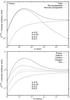Fig. 1 Top: proton spectrum showing the re-accelerated and the normal components. Bottom: re-acceleration effect on different elements. Lines top to bottom: proton, helium, carbon, oxygen, and iron. Model parameters used: η = 0.6, D0 = 5 × 1028 cm2 s-1, ρ0 = 3 GV, a = 0.33, q = 2.3, s = 4.0, and pc = ∞.

The effect of reacceleration on different types of nuclei (proton, helium, carbon, oxygen, and iron) is shown in the bottom panel of Fig. 1. The results shown are for the same set of model parameters used in the top panel of Fig. 1. It can be seen that the reacceleration effect is more prominent for lighter nuclei than for heavier nuclei. It is maximal for protons, and minimal for iron nuclei. In other words, in the present model, light nuclei will show larger GeV-TeV spectral differences than heavy nuclei. For heavier nuclei, because of their larger interaction cross-section, inelastic collisions dominate over reacceleration. But, for lighter nuclei, such as proton and helium, for which the inelastic cross-sections are relatively small, they can be efficiently re-accelerated during their residence time in the Galaxy. This decreasing effect of reacceleration for an increasing elemental mass is expected only in the present model.

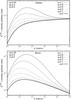Fig. 2 Carbon (top) and boron (bottom) spectra for η = (0,0.1,0.3,0.5,0.8,1.1). Other model parameters remain the same as in Fig. 1.

In Fig. 2, the carbon (top panel) and boron (bottom panel) energy spectra, calculated using Eqs. (7) and (9) respectively, are shown as function of kinetic energy/nucleon. The results are calculated at z = 0, and correspond to different levels of reacceleration given by the parameter η taken in the range of η = 0 − 1.1. The thick solid line represents no reacceleration, i.e., η = 0, and the thin lines correspond to some finite amount of reacceleration with larger η corresponding to higher level of reacceleration. Other model parameters are taken to be the same as in Fig. 1. For the calculation of the boron spectrum, the source parameters are taken to be the same for both the carbon and oxygen nuclei. As η takes larger values, the spectral bump due to reacceleration increases as expected, and at the same time the reacceleration effect becomes extended to higher and higher energies. For η = 1.1, the maximum value considered here, the effect is observed up to a few TeV/n in the carbon spectrum.

Compared to the carbon spectrum, the reacceleration effect is found to be more prominent and more extended in energy in the case of boron. There is some mild effect because of the slightly lower inelastic cross-section of boron nuclei with respect to the carbon that makes the reacceleration more efficient for boron, but this effect is negligible. The main effect, as mentioned in Sect. 2, is because of the contribution from the reacceleration of boron which are produced by the re-accelerated component of the primary carbon and oxygen nuclei. Moreover, the non re-accelerated (normal) component of boron given by the first term of Eq. (9) is steeper than that of the carbon due to the energy dependent escape of cosmic rays from the Galaxy. It may be noted that the spectrum of the normal secondary component is steeper than that of the primaries by the index of diffusion. This allows the re-accelerated component to dominate to higher energies in the case of boron.

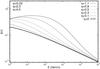Fig. 3 Boron-to-carbon ratio for η = (0,0.1,0.3,0.5,0.8,1.1). Other model parameters are the same as in Fig. 1.

Figure 3 shows the boron-to-carbon ratio for the different values of η. The model parameters and the line representations remain the same as in Fig. 2. Similar effects observed in the energy spectra shown in Fig. 2 are also observed in the ratio. In the model without reacceleration (η = 0), the ratio follows an inverse relation with the diffusion coefficient, and hence, the slope of the ratio follows the inverse of the diffusion index as E^{− a} (see thick solid line in Fig. 3). When comparing the result for η = 0 with the results obtained for η> 0, it is clear that in the reacceleration model, the secondary-to-primary ratio does not represent a direct measure of the cosmic-ray diffusion coefficient in the Galaxy as in pure diffusion models. The ratio also depends on the reacceleration parameters such as the efficiency of reacceleration and the spectral index of the re-accelerated particles s. Moreover, the ratio depends weakly on the primary source parameters such as q and f, unlike in the pure diffusion models where the ratio is almost independent of the source parameters.

3.2. Comparison with the data

For the rest of the study, we take the size of the source distribution R = 20 kpc, the proton high-momentum cutoff p_c = 1 PeV/c, and the supernova explosion rate as  SNe Myr^-1 kpc^-1. The latter corresponds to a rate of ~3 SNe per century in the Galaxy. The cosmic-ray propagation parameters (D₀,ρ₀,a), the reacceleration parameters (η,s), and the source parameters (q,f) are taken as model parameters. They are derived from the measured cosmic-ray data.

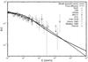Fig. 4 Boron-to-carbon ratio. Solid line: our present result for maximum reacceleration. Dashed line: best-fit result for pure diffusion model (Thoudam & Hörandel 2013). Model parameters used: η = 1.02, D0 = 9 × 1028 cm2 s-1, ρ0 = 3 GV, a = 0.33, qC = 2.24, qO = 2.26, s = 4.5, pc = 1 PeV/c, fC = 0.024%, fO = 0.025%, SNe Myr-1 kpc-2 and φ = 450 MV. Data: HEAO (Engelmann et al. 1990), CRN (Swordy et al. 1990), CREAM (Ahn et al. 2008), AMS-01 (Aguilar et al. 2010), ATIC (Panov et al. 2008; Orth et al. 1978; Simon et al. 1980; Webber et al. 1985), and TRACER (Obermeier et al. 2011).

We first determine (D₀,ρ₀,a,η,s) based on the measurements of the boron-to-carbon ratio, and the spectra for the carbon, oxygen, and boron nuclei simultaneously. Their values are found to be D₀ = 9 × 10²⁸ cm² s^-1, ρ = 3 GV, a = 0.33, η = 1.02, and s = 4.5. These values correspond to the maximum amount of reacceleration permitted by the available boron-to-carbon data, while at the same time produce a reasonably good fit to the measured carbon, oxygen, and boron energy spectra simultaneously. Figure 4 shows the result on the boron-to-carbon ratio (solid line) along with the measurement data. The data are from High Energy Astronomy Observatory Program (HEAO: Engelmann et al. 1990), Cosmic Ray Nuclei Experiment (CRN; Swordy et al. 1990), CREAM (Ahn et al. 2008), Alpha Magnetic Spectrometer (AMS-01; Aguilar et al. 2010), ATIC (Panov et al. 2008; Orth et al. 1978; Simon et al. 1980; Webber et al. 1985), and TRACER (Obermeier et al. 2011). For comparison, we have also shown the best-fit result for the case of pure diffusion (dashed line), i.e., without reacceleration (η = 0), taken from Thoudam & Hörandel (2013). The diffusion index of a = 0.33 obtained in the present model is the same as that found in models of cosmic-ray distributed reacceleration due to interstellar turbulence (Strong & Moskalenko 1998). However, the value of D₀ obtained here is slightly larger than that obtained in Strong & Moskalenko (1998) which gave a value of 7.7 × 10²⁸ cm² s^-1 for the same value of H = 5 kpc.

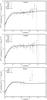Fig. 5 Carbon, oxygen and boron energy spectra. Solid line: our calculation. Model parameters are the same as in Fig. 4. Data: CREAM (Ahn et al. 2009), ATIC (Panov et al. 2007), CRN (Müller et al. 1991; Swordy et al. 1990), HEAO (Engelmann et al. 1990), and TRACER (Obermeier et al. 2011).

The corresponding results on carbon, oxygen, and boron energy spectra are shown in Fig. 5. The solid line represents our results, and the data are taken from CREAM (Ahn et al. 2009), ATIC (Panov et al. 2007), CRN (Müller et al. 1991; Swordy et al. 1990), HEAO (Engelmann et al. 1990), and TRACER (Obermeier et al. 2011). The carbon and oxygen source parameters used are (q_C = 2.24,f_C = 0.024%), and (q_O = 2.26, f_O = 0.025%) respectively, where the f’s are given in units of 10⁵¹ ergs. Our calculation assumes a force-field solar modulation parameter of φ = 450 MV. Our model does not produce a significant spectral hardening for both the carbon and the oxygen spectra although a slight hardening is noticed above ~100 GeV/n in the case of carbon. Given the large uncertainties on the measurements above ~1 TeV/n, our predictions are found to be in agreement with the data up to ~10 TeV/n. For boron nuclei, our model predicts a noticeable spectral hardening above ~500 GeV/n, which is because of the increase in the effect of reacceleration on the secondaries relative to the primaries as discussed above. A similar effect is also visible in the boron-to-carbon ratio shown in Fig. 4 (see solid line). Our prediction is different from that of both the pure diffusion, and the distributed reacceleration models, which predict spectra close to a pure power-law at energies above ~20 − 30 GeV/n. Although our model does not effectively reproduce the highest data point measured by the TRACER experiment, it seems to be consistent with the apparent spectral hardening indicated by the measurement. It can be mentioned that such a hardening in the secondary spectrum can also be attributed to additional components of cosmic-ray secondaries that might exist in the Galaxy and have not been considered in the present model, such as those produced by the interaction of primaries inside the sources or those that result from the reacceleration of background secondaries by strong shocks (see, e.g., Berezhko et al. 2003; Wandel et al. 1987). Such secondaries, although expected to represent a small fraction at low energies, might become important at high energies above ~1 TeV/n because of their harder energy spectrum compared to the secondaries produced in the interstellar medium.

Using the same values of (D₀,ρ₀,a,η,s) obtained above, we calculate the spectra for the proton and helium nuclei. The results are shown in Fig. 6, where the top panel represents proton and the bottom panel represents helium. The lines represent our results, and the data are taken from the CREAM (Yoon et al. 2011), ATIC (Panov et al. 2007), AMS-01 (Alcaraz et al. 2000; Aguilar et al. 2002), and PAMELA (Adriani et al. 2011) experiments. The source parameters used are (q_p = 2.21,f_p = 6.95%) for protons, and (q_He = 2.18,f_He = 0.79%) for helium, and we use the same solar modulation parameter as given above. Our results are in good agreement with the measured data and explain the observed spectral anomaly between the GeV and TeV energy regions. Below ~200 GeV/n, our model spectrum is dominated by the re-accelerated component while above, it is dominated by the normal component. The spectral roll-off above ~10⁵ GeV/n is due to the assumed exponential cutoff of the source spectrum at p_c which we keep fixed at 10⁶ GeV/c for protons.

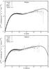Fig. 6 Result for protons (top) and helium nuclei (bottom). Solid line: our calculation. Model parameters used: qP = 2.21, qHe = 2.18, fP = 6.95%, fHe = 0.79%. The propagation and the reacceleration model parameters (D0,ρ0,a,η,s) are the same as in Fig. 4. Data: CREAM (Yoon et al. 2011), ATIC (Panov et al. 2007), AMS-01 (Alcaraz et al. 2000; Aguilar et al. 2002), and PAMELA (Adriani et al. 2011).

Our result shows that the reacceleration effect is stronger in the case of protons resulting into more prominent spectral differences in the GeV-TeV region for protons than for helium. This is partly due to the effect of larger inelastic collision losses for helium nuclei than protons as shown in Fig. 1 (right panel). For the present set of model parameters, there is also an additional effect due to the steeper proton source index of q_p = 2.21 compared to that of helium nuclei of q_He = 2.18. Choosing a larger index produces a steeper spectrum of background cosmic rays in the Galaxy. This leads to two effects on the re-accelerated component. First, a larger number of low-energy background particles become available for reacceleration, leading to an increase in the number of re-accelerated particles. Second, because now the normal component also becomes steeper, the contribution of the re-acelerated component becomes more extended to higher energies. Therefore, the reacceleration effect turns out to be more prominent, and also somewhat more extended in energy for protons than for helium.

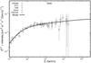Fig. 7 Result for iron nuclei. Solid line: our calculation. Model parameters used: qFe = 2.28, fFe = 0.0049%. All other model parameters remain the same as in Fig. 4. Data: CREAM (Ahn et al. 2009), ATIC (Panov et al. 2007), CRN (Swordy et al. 1990), HEAO (Engelmann et al. 1990), and TRACER (Obermeier et al. 2011).

For heavier nuclei for which the inelastic cross-sections are much larger, the reacceleration effect is significantly less. This is demonstrated in Fig. 7 with our result on the iron nuclei. The calculation assumes the source parameters to be q_Fe = 2.28 and f_Fe = 4.9 × 10^-3% to reproduce the measured spectrum. The propagation and the reacceleration model parameters (D₀,ρ₀,a,η,s) are taken to be the same as in Fig. 4. Even for the steeper source spectrum assumed for the iron nuclei as compared to the proton and helium nuclei, the reacceleration effect is hard to notice in Fig. 7, and the model spectrum above ~20 GeV/n follows approximately a single power law, unlike the proton and helium spectra. Thus, our present model predicts a mass dependent spectral hardening, which can be used to differentiate it from other models in the future. Furthermore, in our model, such a spectral hardening is not expected for electrons as they suffer severe radiative losses that will dominate the reacceleration effect even at few GeV energies.

4. Conclusion

In short, we conclude that the spectral anomaly of cosmic rays at GeV-TeV energies, observed for the proton and helium nuclei by recent experiments, can be an effect of reacceleration of cosmic rays by weak shocks associated with old supernova remnants in the Galaxy. The reacceleration effect is shown to be important for light nuclei such as proton and helium, and negligible for heavier nuclei such as iron. Our prediction of the decreasing effect of reacceleration with the increase in the elemental mass can be checked by future sensitive measurements of heavier nuclei at TeV/n energies. The reacceleration effect is expected to be negligible for electrons.

Online material

Appendix A: Derivation of Green’s function for Eq. (1)

The Green’s function G(r,r′,p,p′) for Eq. (1) satisfies $\begin{array}{ccc}\mathrm{\nabla }\mathrm{·}\mathrm{\left(}\mathit{D}\mathrm{\nabla }\mathit{G}\mathrm{\right)}& \mathrm{-}& \left[\mathit{n̅}\mathit{v\sigma }\mathrm{+}\mathit{\xi }\right]\mathit{\delta }\mathrm{\left(}\mathit{z}\mathrm{\right)}\mathit{G}\mathrm{+}\left[\mathit{\xi s}{\mathit{p}}^{\mathrm{-}\mathit{s}}{\mathrm{\int }}_{{\mathit{p}}_{\mathrm{0}}}^{\mathit{p}}\mathrm{d}\mathit{uG}\mathrm{\left(}\mathit{u}\mathrm{\right)}{\mathit{u}}^{\mathit{s}\mathrm{-}\mathrm{1}}\right]\mathit{\delta }\mathrm{\left(}\mathit{z}\mathrm{\right)}\mathrm{=}\\ & & \mathrm{-}\mathit{\delta }\mathrm{(}{r}\mathrm{-}{{r}}^{\mathrm{\prime }}\mathrm{)}\mathit{\delta }\mathrm{(}\mathit{p}\mathrm{-}{\mathit{p}}^{\mathrm{\prime }}\mathrm{)}\end{array}$(A.1)where G(u) ≡ G(r,r′,u,p′). In rectangular coordinates, and assuming the sources are on the Galactic plane, i.e., z′ = 0, we can write the above equation as

$\begin{array}{ccc}& & \mathit{D}\frac{{\mathit{\partial }}^{\mathrm{2}}\mathit{G}}{\mathit{\partial }{\mathit{x}}^{\mathrm{2}}}\mathrm{+}\mathit{D}\frac{{\mathit{\partial }}^{\mathrm{2}}\mathit{G}}{\mathit{\partial }{\mathit{y}}^{\mathrm{2}}}\mathrm{+}\mathit{D}\frac{{\mathit{\partial }}^{\mathrm{2}}\mathit{G}}{\mathit{\partial }{\mathit{z}}^{\mathrm{2}}}\mathrm{-}\left[\mathit{n̅}\mathit{v\sigma }\mathrm{+}\mathit{\xi }\right]\mathit{\delta }\mathrm{\left(}\mathit{z}\mathrm{\right)}\mathit{G}\\ & & \mathrm{+}\left[\mathit{\xi s}{\mathit{p}}^{\mathrm{-}\mathit{s}}{\mathrm{\int }}_{{\mathit{p}}_{\mathrm{0}}}^{\mathit{p}}\mathrm{d}\mathit{uG}\mathrm{\left(}\mathit{u}\mathrm{\right)}{\mathit{u}}^{\mathit{s}\mathrm{-}\mathrm{1}}\right]\mathit{\delta }\mathrm{\left(}\mathit{z}\mathrm{\right)}\mathrm{=}\mathrm{-}\mathit{\delta }\mathrm{(}\mathit{x}\mathrm{-}{\mathit{x}}^{\mathrm{\prime }}\mathrm{)}\mathit{\delta }\mathrm{(}\mathit{y}\mathrm{-}{\mathit{y}}^{\mathrm{\prime }}\mathrm{)}\mathit{\delta }\mathrm{\left(}\mathit{z}\mathrm{\right)}\mathit{\delta }\mathrm{(}\mathit{p}\mathrm{-}{\mathit{p}}^{\mathrm{\prime }}\mathrm{)}\mathit{.}\end{array}$(A.2)After taking Fourier transform of Eq. (A.2) with respect to x and y, we have

$\begin{array}{ccc}& & \mathrm{-}\mathit{D}{\mathit{k}}^{\mathrm{2}}\mathit{G̅}\mathrm{+}\mathit{D}\frac{{\mathit{\partial }}^{\mathrm{2}}\mathit{G̅}}{\mathit{\partial }{\mathit{z}}^{\mathrm{2}}}\mathrm{-}\left[\mathit{n̅}\mathit{v\sigma }\mathrm{+}\mathit{\xi }\right]\mathit{\delta }\mathrm{\left(}\mathit{z}\mathrm{\right)}\mathit{G̅}\mathrm{+}\left[\mathit{\xi s}{\mathit{p}}^{\mathrm{-}\mathit{s}}{\mathrm{\int }}_{{\mathit{p}}_{\mathrm{0}}}^{\mathit{p}}\mathrm{d}\mathit{u}\mathit{G̅}\mathrm{\left(}\mathit{u}\mathrm{\right)}{\mathit{u}}^{\mathit{s}\mathrm{-}\mathrm{1}}\right]\\ & & \mathit{\delta }\mathrm{\left(}\mathit{z}\mathrm{\right)}\mathrm{=}\mathrm{-}\exp \mathrm{(}\mathrm{i}{\mathit{k}}_{\mathit{x}}{\mathit{x}}^{\mathrm{\prime }}\mathrm{+}\mathrm{i}{\mathit{k}}_{\mathit{y}}{\mathit{y}}^{\mathrm{\prime }}\mathrm{)}\mathit{\delta }\mathrm{\left(}\mathit{z}\mathrm{\right)}\mathit{\delta }\mathrm{(}\mathit{p}\mathrm{-}{\mathit{p}}^{\mathrm{\prime }}\mathrm{)}\end{array}$(A.3)where ${\mathit{k}}^{\mathrm{2}}\mathrm{=}{\mathit{k}}_{\mathit{x}}^{\mathrm{2}}\mathrm{+}{\mathit{k}}_{\mathit{y}}^{\mathrm{2}}$, and

$\begin{array}{ccc}& & \mathit{G̅}\mathrm{\left(}{\mathit{k}}_{\mathit{x}}\mathit{,}{\mathit{x}}^{\mathrm{\prime }}\mathit{,}{\mathit{k}}_{\mathit{y}}\mathit{,}{\mathit{y}}^{\mathrm{\prime }}\mathit{,z,p,}{\mathit{p}}^{\mathrm{\prime }}\mathrm{\right)}\mathrm{=}\\ & & {\mathrm{\int }}_{\mathrm{-}\mathrm{\infty }}^{\mathrm{\infty }}\mathrm{d}\mathit{x}{\mathrm{\int }}_{\mathrm{-}\mathrm{\infty }}^{\mathrm{\infty }}\mathrm{d}\mathit{yG}\mathrm{\left(}\mathit{x,}{\mathit{x}}^{\mathrm{\prime }}\mathit{,y,}{\mathit{y}}^{\mathrm{\prime }}\mathit{,z,p,}{\mathit{p}}^{\mathrm{\prime }}\mathrm{\right)}\exp \mathrm{(}\mathrm{i}{\mathit{k}}_{\mathit{x}}\mathit{x}\mathrm{+}\mathrm{i}{\mathit{k}}_{\mathit{y}}\mathit{y}\mathrm{)}\mathit{.}\end{array}$For z ≠ 0, Eq. (A.3) reduces to the following simple differential equation: $\mathrm{-}\mathit{D}{\mathit{k}}^{\mathrm{2}}\mathit{G̅}\mathrm{+}\mathit{D}\frac{{\mathit{\partial }}^{\mathrm{2}}\mathit{G̅}}{\mathit{\partial }{\mathit{z}}^{\mathrm{2}}}\mathrm{=}\mathrm{0.}$(A.4)Solving the above equation by using the boundary condition that the particle density, and hence , vanishes at z = ± H, the solution of Eq. (A.3) for regions above (z> 0) and below (z< 0) the Galactic plane is obtained as, $\mathit{G̅}\mathrm{\left(}{\mathit{k}}_{\mathit{x}}\mathit{,}{\mathit{x}}^{\mathrm{\prime }}\mathit{,}{\mathit{k}}_{\mathit{y}}\mathit{,}{\mathit{y}}^{\mathrm{\prime }}\mathit{,z,p,}{\mathit{p}}^{\mathrm{\prime }}\mathrm{\right)}\mathrm{=}\mathit{G̅}\mathrm{\left(}\mathrm{0}\mathrm{\right)}\frac{\sinh \left[\mathit{k}\mathrm{(}\mathit{H}\mathrm{-}\mathrm{|}\mathit{z}\mathrm{\left|}\mathrm{\right)}\right]}{\sinh \mathrm{\left(}\mathit{kH}\mathrm{\right)}}$(A.5)where . The function can be determined using the continuity relation at z = 0 as follows. Integrating Eq. (A.3) over z around z = 0, we get

$\begin{array}{ccc}& & {\mathit{D}\frac{\mathit{\partial }\mathit{G̅}}{\mathit{\partial z}}|}_{\mathit{z}\mathrm{=}\mathrm{0}\mathrm{+}}\mathrm{-}{\mathit{D}\frac{\mathit{\partial }\mathit{G̅}}{\mathit{\partial z}}|}_{\mathit{z}\mathrm{=}\mathrm{0}\mathrm{-}}\mathrm{-}\left[\mathit{n̅}\mathit{v\sigma }\mathrm{+}\mathit{\xi }\right]\mathit{G̅}\mathrm{\left(}\mathrm{0}\mathrm{\right)}\\ & & \mathrm{+}\left[\mathit{\xi s}{\mathit{p}}^{\mathrm{-}\mathit{s}}{\mathrm{\int }}_{{\mathit{p}}_{\mathrm{0}}}^{\mathit{p}}\mathrm{d}\mathit{u}\mathit{G̅}\mathrm{\left(}\mathrm{0}\mathit{,u}\mathrm{\right)}{\mathit{u}}^{\mathit{s}\mathrm{-}\mathrm{1}}\right]\mathrm{=}\mathrm{-}\exp \mathrm{(}\mathrm{i}{\mathit{k}}_{\mathit{x}}{\mathit{x}}^{\mathrm{\prime }}\mathrm{+}\mathrm{i}{\mathit{k}}_{\mathit{y}}{\mathit{y}}^{\mathrm{\prime }}\mathrm{)}\mathit{\delta }\mathrm{(}\mathit{p}\mathrm{-}{\mathit{p}}^{\mathrm{\prime }}\mathrm{)}\end{array}$(A.6)where . Substituting for at z = 0 ±, and rearranging the terms, Eq. (A.5) reduces into a first order linear differential equation in p as $\frac{\mathrm{d}\mathit{G̅}\mathrm{\left(}\mathrm{0}\mathrm{\right)}}{\mathrm{d}\mathit{p}}\mathrm{+}\mathit{A}\mathrm{\left(}\mathit{p}\mathrm{\right)}\mathit{G̅}\mathrm{\left(}\mathrm{0}\mathrm{\right)}\mathrm{=}\mathrm{-}\mathit{B}\mathrm{\left(}\mathit{p}\mathrm{\right)}$(A.7)where, $\begin{array}{ccc}& & \mathit{A}\mathrm{\left(}\mathit{p}\mathrm{\right)}\mathrm{=}\frac{\mathit{s}}{\mathit{p}}\mathrm{-}\frac{\mathit{\xi s}}{\mathit{pL}\mathrm{\left(}\mathit{p}\mathrm{\right)}}\mathrm{+}\frac{\mathrm{1}}{\mathit{L}\mathrm{\left(}\mathit{p}\mathrm{\right)}}\frac{\mathrm{d}}{\mathrm{d}\mathit{p}}\mathit{L}\mathrm{\left(}\mathit{p}\mathrm{\right)}\mathit{,}\\ & & \mathit{L}\mathrm{\left(}\mathit{p}\mathrm{\right)}\mathrm{=}\mathrm{2}\mathit{D}\mathrm{\left(}\mathit{p}\mathrm{\right)}\mathit{k}\coth \mathrm{\left(}\mathit{kH}\mathrm{\right)}\mathrm{+}\mathit{n̅}\mathit{v}\mathrm{\left(}\mathit{p}\mathrm{\right)}\mathit{\sigma }\mathrm{\left(}\mathit{p}\mathrm{\right)}\mathrm{+}\mathit{\xi ,}\\ & & \mathit{B}\mathrm{\left(}\mathit{p}\mathrm{\right)}\mathrm{=}\mathrm{-}\frac{\mathit{C}\mathrm{\left(}\mathit{p}\mathrm{\right)}}{{\mathit{p}}^{\mathit{s}}}\frac{\mathrm{d}}{\mathrm{d}\mathit{p}}\left[{\mathit{p}}^{\mathit{s}}\mathit{\delta }\mathrm{(}\mathit{p}\mathrm{-}{\mathit{p}}^{\mathrm{\prime }}\mathrm{)}\right]\mathit{,}\mathrm{and}\\ & & \mathit{C}\mathrm{\left(}\mathit{p}\mathrm{\right)}\mathrm{=}\frac{\exp \mathrm{(}\mathrm{i}{\mathit{k}}_{\mathit{x}}{\mathit{x}}^{\mathrm{\prime }}\mathrm{+}\mathrm{i}{\mathit{k}}_{\mathit{y}}{\mathit{y}}^{\mathrm{\prime }}\mathrm{)}}{\mathit{L}\mathrm{\left(}\mathit{p}\mathrm{\right)}}\mathrm{·}\end{array}$(A.8)The integrating factor of Eq. (A.6) is: $\mathit{I}\mathit{.}\mathit{F}\mathrm{=}\exp \left({\mathrm{\int }}^{\mathit{p}}\mathit{A}\mathrm{\left(}\mathit{u}\mathrm{\right)}\mathrm{d}\mathit{u}\right)\mathit{.}$(A.9)With this, the general solution of Eq. (A.6) is obtained as, $\begin{array}{ccc}& & \mathit{G̅}\mathrm{\left(}\mathrm{0}\mathrm{\right)}\mathrm{\times }\exp \left({\mathrm{\int }}^{\mathit{p}}\mathit{A}\mathrm{\left(}\mathit{u}\mathrm{\right)}\mathrm{d}\mathit{u}\right)\mathrm{=}\\ & & \mathrm{-}{\mathrm{\int }}^{\mathit{p}}\mathrm{d}{\mathit{p}}_{\mathrm{1}}\mathit{B}\mathrm{\left(}{\mathit{p}}_{\mathrm{1}}\mathrm{\right)}\exp \left({\mathrm{\int }}^{{\mathit{p}}_{\mathrm{1}}}\mathit{A}\mathrm{\left(}\mathit{u}\mathrm{\right)}\mathrm{d}\mathit{u}\right)\mathrm{+}{\mathit{I}}_{\mathrm{0}}\mathit{,}\\ & \mathrm{where}{\mathit{I}}_{\mathrm{0}}\mathrm{istheintegrationconstant}& \\ & \mathrm{=}& \mathrm{-}{\mathrm{\int }}^{\mathit{p}}\mathrm{d}{\mathit{p}}_{\mathrm{1}}\frac{\mathrm{-}\mathit{C}\mathrm{\left(}{\mathit{p}}_{\mathrm{1}}\mathrm{\right)}}{{\mathit{p}}_{\mathrm{1}}^{\mathit{s}}}\frac{\mathrm{d}}{\mathrm{d}{\mathit{p}}_{\mathrm{1}}}\mathrm{\left[}{\mathit{p}}_{\mathrm{1}}^{\mathit{s}}\mathit{\delta }\mathrm{\right(}{\mathit{p}}_{\mathrm{1}}\mathrm{-}{\mathit{p}}^{\mathrm{\prime }}\mathrm{\left)}\mathrm{\right]}\exp \left({\mathrm{\int }}^{{\mathit{p}}_{\mathrm{1}}}\mathit{A}\mathrm{\left(}\mathit{u}\mathrm{\right)}\mathrm{d}\mathit{u}\right)\mathrm{+}{\mathit{I}}_{\mathrm{0}}\\ & \mathrm{=}& \mathrm{-}{\mathrm{\int }}^{\mathit{p}}\mathrm{d}{\mathit{p}}_{\mathrm{1}}\mathit{E}\mathrm{\left(}{\mathit{p}}_{\mathrm{1}}\mathrm{\right)}\frac{\mathrm{d}}{\mathrm{d}{\mathit{p}}_{\mathrm{1}}}\mathrm{\left[}{\mathit{p}}_{\mathrm{1}}^{\mathit{s}}\mathit{\delta }\mathrm{\right(}{\mathit{p}}_{\mathrm{1}}\mathrm{-}{\mathit{p}}^{\mathrm{\prime }}\mathrm{\left)}\mathrm{\right]}\mathrm{+}{\mathit{I}}_{\mathrm{0}}\end{array}$(A.10)where we have written,

$\mathit{E}\mathrm{\left(}{\mathit{p}}_{\mathrm{1}}\mathrm{\right)}\mathrm{=}\mathrm{-}\frac{\mathit{C}\mathrm{\left(}{\mathit{p}}_{\mathrm{1}}\mathrm{\right)}}{{{\mathit{p}}_{\mathrm{1}}}^{\mathit{s}}}\exp \left({\mathrm{\int }}^{{\mathit{p}}_{\mathrm{1}}}\mathit{A}\mathrm{\left(}\mathit{u}\mathrm{\right)}\mathrm{d}\mathit{u}\right)\mathit{.}$(A.11)The first term on the right hand side of Eq. (A.8) can be integrated by parts taking E(p₁) as the first function and the derivative part as the second function as follows: $\begin{array}{ccc}\mathit{G̅}\mathrm{\left(}\mathrm{0}\mathrm{\right)}& \mathrm{\times }& \exp \left({\mathrm{\int }}^{\mathit{p}}\mathit{A}\mathrm{\left(}\mathit{u}\mathrm{\right)}\mathrm{d}\mathit{u}\right)\mathrm{=}\mathrm{-}\mathit{E}\mathrm{\left(}\mathit{p}\mathrm{\right)}{\mathit{p}}^{\mathit{s}}\mathit{\delta }\mathrm{(}\mathit{p}\mathrm{-}{\mathit{p}}^{\mathrm{\prime }}\mathrm{)}\\ & \mathrm{+}{\mathrm{\int }}^{\mathit{p}}\mathrm{d}{\mathit{p}}_{\mathrm{1}}{\mathit{p}}_{\mathrm{1}}^{\mathit{s}}\mathit{\delta }\mathrm{(}{\mathit{p}}_{\mathrm{1}}\mathrm{-}{\mathit{p}}^{\mathrm{\prime }}\mathrm{)}\frac{\mathrm{d}}{\mathrm{d}{\mathit{p}}_{\mathrm{1}}}\mathit{E}\mathrm{\left(}{\mathit{p}}_{\mathrm{1}}\mathrm{\right)}\mathrm{+}{\mathit{I}}_{\mathrm{0}}\mathrm{=}& \\ & \mathrm{-}& \mathit{E}\mathrm{\left(}\mathit{p}\mathrm{\right)}{\mathit{p}}^{\mathit{s}}\mathit{\delta }\mathrm{(}\mathit{p}\mathrm{-}{\mathit{p}}^{\mathrm{\prime }}\mathrm{)}\mathrm{+}\mathrm{H}\mathrm{[}\mathit{p}\mathrm{-}{\mathit{p}}^{\mathrm{\prime }}\mathrm{]}{{\mathit{p}}^{\mathrm{\prime }}}^{\mathit{s}}\frac{\mathrm{d}}{\mathrm{d}{\mathit{p}}^{\mathrm{\prime }}}\mathit{E}\mathrm{\left(}{\mathit{p}}^{\mathrm{\prime }}\mathrm{\right)}\mathrm{+}{\mathit{I}}_{\mathrm{0}}\end{array}$(A.12)where H[m] is the Heaviside step function, which has the property H[m] = 1(0) for m> 0( < 0). Substituting for E(p), which is defined by Eq. (A.9), into Eq. (A.10), we get, $\begin{array}{ccc}\mathit{G̅}\mathrm{\left(}\mathrm{0}\mathrm{\right)}\mathrm{\times }\exp \left({\mathrm{\int }}^{\mathit{p}}\mathit{A}\mathrm{\left(}\mathit{u}\mathrm{\right)}\mathrm{d}\mathit{u}\right)& \mathrm{=}\mathit{C}\mathrm{\left(}\mathit{p}\mathrm{\right)}\mathit{\delta }\mathrm{(}\mathit{p}\mathrm{-}{\mathit{p}}^{\mathrm{\prime }}\mathrm{)}\exp {\mathrm{(}}^{\mathrm{\int }}\mathit{p}\mathit{A}\mathrm{\left(}\mathit{u}\mathrm{\right)}\mathrm{d}{\mathit{u}}^{\mathrm{)}}& \\ & \mathrm{+}\mathrm{H}\mathrm{[}\mathit{p}\mathrm{-}{\mathit{p}}^{\mathrm{\prime }}\mathrm{]}{{\mathit{p}}^{\mathrm{\prime }}}^{\mathit{s}}\frac{\mathrm{d}}{\mathrm{d}{\mathit{p}}^{\mathrm{\prime }}}\mathit{E}\mathrm{\left(}{\mathit{p}}^{\mathrm{\prime }}\mathrm{\right)}\mathrm{+}{\mathit{I}}_{\mathrm{0}}\mathit{.}& \end{array}$(A.13)Imposing the boundary condition that there are no particles at p = 0, Eq. (A.11) becomes,

$\mathrm{0}\mathrm{=}\mathit{C}\mathrm{\left(}\mathrm{0}\mathrm{\right)}\mathit{\delta }\mathrm{(}\mathrm{0}\mathrm{-}{\mathit{p}}^{\mathrm{\prime }}\mathrm{)}\exp \left({\mathrm{\int }}^{\mathit{p}\mathrm{=}\mathrm{0}}\mathit{A}\mathrm{\left(}\mathit{u}\mathrm{\right)}\mathrm{d}\mathit{u}\right)\mathrm{+}\mathrm{H}\mathrm{[}\mathrm{0}\mathrm{-}{\mathit{p}}^{\mathrm{\prime }}\mathrm{]}{{\mathit{p}}^{\mathrm{\prime }}}^{\mathit{s}}\frac{\mathrm{d}}{\mathrm{d}{\mathit{p}}^{\mathrm{\prime }}}\mathit{E}\mathrm{\left(}{\mathit{p}}^{\mathrm{\prime }}\mathrm{\right)}\mathrm{+}{\mathit{I}}_{\mathrm{0}}\mathit{.}$(A.14)In the present study, as we assume that particles are injected with a finite momentum p′ ≥ p₀ where p₀ is the low-momentum cutoff we have introduced so as to approximate the ionization losses (see Sect. 2), the delta function and the Heaviside step function in the first two terms on the right hand side of the above equation becomes zero. This gives I₀ = 0, and the general solution of Eq. (A.6) becomes, $\mathit{G̅}\mathrm{\left(}\mathrm{0}\mathrm{\right)}\mathrm{=}\mathit{C}\mathrm{\left(}\mathit{p}\mathrm{\right)}\mathit{\delta }\mathrm{(}\mathit{p}\mathrm{-}{\mathit{p}}^{\mathrm{\prime }}\mathrm{)}\mathrm{+}\mathrm{H}\mathrm{[}\mathit{p}\mathrm{-}{\mathit{p}}^{\mathrm{\prime }}\mathrm{]}{{\mathit{p}}^{\mathrm{\prime }}}^{\mathit{s}}\frac{\mathrm{d}}{\mathrm{d}{\mathit{p}}^{\mathrm{\prime }}}\mathit{E}\mathrm{\left(}{\mathit{p}}^{\mathrm{\prime }}\mathrm{\right)}\exp \left(\mathrm{-}{\mathrm{\int }}^{\mathit{p}}\mathit{A}\mathrm{\left(}\mathit{u}\mathrm{\right)}\mathrm{d}\mathit{u}\right)\mathit{.}$(A.15)Proceeding further, we have,

$\begin{array}{ccc}\mathrm{\int }\mathit{A}\mathrm{\left(}\mathit{u}\mathrm{\right)}\mathit{du}& \mathrm{=}& \int \mathrm{d}\mathit{u}\left(\frac{\mathit{s}}{\mathit{u}}\mathrm{-}\frac{\mathit{s\xi }}{\mathit{uL}\mathrm{\left(}\mathit{u}\mathrm{\right)}}\mathrm{+}\frac{\mathrm{1}}{\mathit{L}\mathrm{\left(}\mathit{u}\mathrm{\right)}}\frac{\mathrm{d}}{\mathrm{d}\mathit{u}}\mathit{L}\mathrm{\left(}\mathit{u}\mathrm{\right)}\right)\\ & \mathrm{=}& \ln {\mathit{u}}^{\mathit{s}}\mathrm{+}\mathit{\xi s}\mathrm{\int }\mathit{I}\mathrm{\left(}\mathit{u}\mathrm{\right)}\mathrm{d}\mathit{u}\mathrm{+}\ln \mathit{L}\mathrm{\left(}\mathit{u}\mathrm{\right)}\mathit{,}\\ & \mathrm{wherewehavewritten}\mathit{I}\mathrm{\left(}\mathit{u}\mathrm{\right)}\mathrm{=}\mathrm{-}\frac{\mathrm{1}}{\mathit{uL}\mathrm{\left(}\mathit{u}\mathrm{\right)}}\mathrm{·}& \end{array}$Therefore, we can write

$\begin{array}{ccc}\exp \left(\mathrm{\int }\mathit{A}\mathrm{\left(}\mathit{u}\mathrm{\right)}\mathrm{d}\mathit{u}\right)\mathrm{=}{\mathit{u}}^{\mathit{s}}\mathit{L}\mathrm{\left(}\mathit{u}\mathrm{\right)}\exp \left(\mathit{\xi s}\mathrm{\int }\mathit{I}\mathrm{\left(}\mathit{u}\mathrm{\right)}\mathrm{d}\mathit{u}\right)\mathit{.}& & \end{array}$(A.16)Then, E(p′) defined by Eq. (A.9) becomes,

$\begin{array}{ccc}\mathit{E}\mathrm{\left(}{\mathit{p}}^{\mathrm{\prime }}\mathrm{\right)}\mathrm{=}\mathrm{-}\frac{\mathit{C}\mathrm{\left(}{\mathit{p}}^{\mathrm{\prime }}\mathrm{\right)}}{{{\mathit{p}}^{\mathrm{\prime }}}^{\mathit{s}}}{{\mathit{p}}^{\mathrm{\prime }}}^{\mathit{s}}\mathit{L}\mathrm{\left(}{\mathit{p}}^{\mathrm{\prime }}\mathrm{\right)}\exp \left(\mathit{\xi s}{\mathrm{\int }}^{{\mathit{p}}^{\mathrm{\prime }}}\mathit{I}\mathrm{\left(}\mathit{u}\mathrm{\right)}\mathrm{d}\mathit{u}\right)\mathit{.}& & \end{array}$(A.17)Substituting for C(p′) as defined by Eq. (A.7) into Eq. (A.14), we get $\begin{array}{ccc}\mathit{E}\mathrm{\left(}{\mathit{p}}^{\mathrm{\prime }}\mathrm{\right)}\mathrm{=}\mathrm{-}\exp \mathrm{(}\mathrm{i}{\mathit{k}}_{\mathit{x}}{\mathit{x}}^{\mathrm{\prime }}\mathrm{+}\mathrm{i}{\mathit{k}}_{\mathit{y}}{\mathit{y}}^{\mathrm{\prime }}\mathrm{)}\exp \left(\mathit{\xi s}{\mathrm{\int }}^{{\mathit{p}}^{\mathrm{\prime }}}\mathit{I}\mathrm{\left(}\mathit{u}\mathrm{\right)}\mathrm{d}\mathit{u}\right)\mathit{.}& & \end{array}$(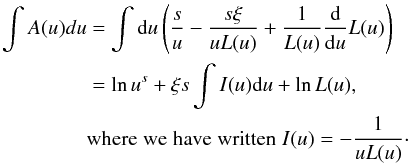A.18)Differentiating Eq. (A.15) with respect to p′, we have

$\begin{array}{ccc}\frac{\mathrm{d}}{\mathrm{d}{\mathit{p}}^{\mathrm{\prime }}}\mathit{E}\mathrm{\left(}{\mathit{p}}^{\mathrm{\prime }}\mathrm{\right)}& \mathrm{=}\mathrm{-}\exp \mathrm{(}\mathrm{i}{\mathit{k}}_{\mathit{x}}{\mathit{x}}^{\mathrm{\prime }}\mathrm{+}\mathrm{i}{\mathit{k}}_{\mathit{y}}{\mathit{y}}^{\mathrm{\prime }}\mathrm{)}\exp \left(\mathit{\xi s}{\mathrm{\int }}^{{\mathit{p}}^{\mathrm{\prime }}}\mathit{I}\mathrm{\left(}\mathit{u}\mathrm{\right)}\mathrm{d}\mathit{u}\right)& \\ & & \hspace{0.17em}\hspace{0.17em}\hspace{0.17em}\mathrm{\times }\frac{\mathrm{d}}{\mathrm{d}{\mathit{p}}^{\mathrm{\prime }}}\left(\mathit{\xi s}{\mathrm{\int }}^{{\mathit{p}}^{\mathrm{\prime }}}\mathit{I}\mathrm{\left(}\mathit{u}\mathrm{\right)}\mathrm{d}\mathit{u}\right)\\ & \mathrm{=}& \mathrm{-}\exp \mathrm{(}\mathrm{i}{\mathit{k}}_{\mathit{x}}{\mathit{x}}^{\mathrm{\prime }}\mathrm{+}\mathrm{i}{\mathit{k}}_{\mathit{y}}{\mathit{y}}^{\mathrm{\prime }}\mathrm{)}\exp \left(\mathit{\xi s}{\mathrm{\int }}^{{\mathit{p}}^{\mathrm{\prime }}}\mathit{I}\mathrm{\left(}\mathit{u}\mathrm{\right)}\mathrm{d}\mathit{u}\right)\mathit{\xi sI}\mathrm{\left(}{\mathit{p}}^{\mathrm{\prime }}\mathrm{\right)}\\ & \mathrm{=}& \exp \mathrm{(}\mathrm{i}{\mathit{k}}_{\mathit{x}}{\mathit{x}}^{\mathrm{\prime }}\mathrm{+}\mathrm{i}{\mathit{k}}_{\mathit{y}}{\mathit{y}}^{\mathrm{\prime }}\mathrm{)}\exp \left(\mathit{\xi s}{\mathrm{\int }}^{{\mathit{p}}^{\mathrm{\prime }}}\mathit{I}\mathrm{\left(}\mathit{u}\mathrm{\right)}\mathrm{d}\mathit{u}\right)\frac{\mathit{\xi s}}{{\mathit{p}}^{\mathrm{\prime }}\mathit{L}\mathrm{\left(}{\mathit{p}}^{\mathrm{\prime }}\mathrm{\right)}}\end{array}$(A.19)where we have substituted $\mathit{I}\mathrm{\left(}{\mathit{p}}^{\mathrm{\prime }}\mathrm{\right)}\mathrm{=}\mathrm{-}\frac{\mathrm{1}}{{\mathit{p}}^{\mathrm{\prime }}\mathit{L}\mathrm{\left(}{\mathit{p}}^{\mathrm{\prime }}\mathrm{\right)}}$ in the last expression. Analogous to Eq. (A.13), we also obtain, $\begin{array}{ccc}\exp \left(\mathrm{-}{\mathrm{\int }}^{\mathit{p}}\mathit{A}\mathrm{\left(}\mathit{u}\mathrm{\right)}\mathrm{d}\mathit{u}\right)\mathrm{=}\frac{\mathrm{1}}{{\mathit{p}}^{\mathit{s}}\mathit{L}\mathrm{\left(}\mathit{p}\mathrm{\right)}}\exp \left(\mathrm{-}\mathit{\xi s}{\mathrm{\int }}^{\mathit{p}}\mathit{I}\mathrm{\left(}\mathit{u}\mathrm{\right)}\mathrm{d}\mathit{u}\right)\mathit{.}& & \end{array}$(A.20)Substituting Eqs. (A.16) and (A.17) into Eq. (A.12), we get $\begin{array}{ccc}\mathit{G̅}\mathrm{\left(}\mathrm{0}\mathrm{\right)}& \mathrm{=}& \mathit{C}\mathrm{\left(}\mathit{p}\mathrm{\right)}\mathit{\delta }\mathrm{(}\mathit{p}\mathrm{-}{\mathit{p}}^{\mathrm{\prime }}\mathrm{)}\mathrm{+}\mathrm{H}\mathrm{[}\mathit{p}\mathrm{-}{\mathit{p}}^{\mathrm{\prime }}\mathrm{]}{{\mathit{p}}^{\mathrm{\prime }}}^{\mathit{s}}\exp \mathrm{(}\mathrm{i}{\mathit{k}}_{\mathit{x}}{\mathit{x}}^{\mathrm{\prime }}\mathrm{+}\mathrm{i}{\mathit{k}}_{\mathit{y}}{\mathit{y}}^{\mathrm{\prime }}\mathrm{)}\frac{\mathit{\xi s}}{{\mathit{p}}^{\mathrm{\prime }}\mathit{L}\mathrm{\left(}{\mathit{p}}^{\mathrm{\prime }}\mathrm{\right)}}\\ & & \mathrm{\times }\exp \left(\mathit{\xi s}{\mathrm{\int }}^{{\mathit{p}}^{\mathrm{\prime }}}\mathit{I}\mathrm{\left(}\mathit{u}\mathrm{\right)}\mathrm{d}\mathit{u}\right)\frac{\mathrm{1}}{{\mathit{p}}^{\mathit{s}}\mathit{L}\mathrm{\left(}\mathit{p}\mathrm{\right)}}\exp \left(\mathrm{-}\mathit{\xi s}{\mathrm{\int }}^{\mathit{p}}\mathit{I}\mathrm{\left(}\mathit{u}\mathrm{\right)}\mathrm{d}\mathit{u}\right)\\ & \mathrm{=}& \mathit{C}\mathrm{\left(}\mathit{p}\mathrm{\right)}\mathit{\delta }\mathrm{(}\mathit{p}\mathrm{-}{\mathit{p}}^{\mathrm{\prime }}\mathrm{)}\mathrm{+}\mathrm{H}\mathrm{[}\mathit{p}\mathrm{-}{\mathit{p}}^{\mathrm{\prime }}\mathrm{]}\frac{\exp \mathrm{(}\mathrm{i}{\mathit{k}}_{\mathit{x}}{\mathit{x}}^{\mathrm{\prime }}\mathrm{+}\mathrm{i}{\mathit{k}}_{\mathit{y}}{\mathit{y}}^{\mathrm{\prime }}\mathrm{)}}{\mathit{L}\mathrm{\left(}\mathit{p}\mathrm{\right)}}\frac{\mathit{\xi s}{{\mathit{p}}^{\mathrm{\prime }}}^{\mathit{s}\mathrm{-}\mathrm{1}}}{{\mathit{p}}^{\mathit{s}}\mathit{L}\mathrm{\left(}{\mathit{p}}^{\mathrm{\prime }}\mathrm{\right)}}\\ & & \mathrm{\times }\exp \left(\mathit{\xi s}{\mathrm{\int }}_{\mathit{p}}^{{\mathit{p}}^{\mathrm{\prime }}}\mathit{I}\mathrm{\left(}\mathit{u}\mathrm{\right)}\mathrm{d}\mathit{u}\right)\\ & \mathrm{=}& \frac{\exp \mathrm{(}\mathrm{i}{\mathit{k}}_{\mathit{x}}{\mathit{x}}^{\mathrm{\prime }}\mathrm{+}\mathrm{i}{\mathit{k}}_{\mathit{y}}{\mathit{y}}^{\mathrm{\prime }}\mathrm{)}}{\mathit{L}\mathrm{\left(}\mathit{p}\mathrm{\right)}}[\mathit{\delta }\mathrm{(}\mathit{p}\mathrm{-}{\mathit{p}}^{\mathrm{\prime }}\mathrm{)}\mathrm{+}\mathrm{H}\mathrm{[}\mathit{p}\mathrm{-}{\mathit{p}}^{\mathrm{\prime }}\mathrm{]}\frac{\mathit{\xi s}{{\mathit{p}}^{\mathrm{\prime }}}^{\mathit{s}\mathrm{-}\mathrm{1}}}{{\mathit{p}}^{\mathit{s}}\mathit{L}\mathrm{\left(}{\mathit{p}}^{\mathrm{\prime }}\mathrm{\right)}}\\ & & \mathrm{\times }\exp \left(\mathit{\xi s}{\mathrm{\int }}_{\mathit{p}}^{{\mathit{p}}^{\mathrm{\prime }}}\mathit{I}\mathrm{\left(}\mathit{u}\mathrm{\right)}\mathrm{d}\mathit{u}\right)]\\ & & \mathrm{wherewehavesubstituted}\mathit{C}\mathit{\left(}\mathit{p}\mathit{\right)}\mathrm{fromEq}\mathit{.}\mathrm{\left(}\mathrm{A}\mathit{.7}\mathrm{\right)}\\ & \mathrm{=}& \exp \mathrm{(}\mathrm{i}{\mathit{k}}_{\mathit{x}}{\mathit{x}}^{\mathrm{\prime }}\mathrm{+}\mathrm{i}{\mathit{k}}_{\mathit{y}}{\mathit{y}}^{\mathrm{\prime }}\mathrm{)}\mathit{F}\mathrm{\left(}\mathit{p,}{\mathit{p}}^{\mathrm{\prime }}\mathrm{\right)}\end{array}$(A.21)where we have written, $\begin{array}{ccc}\mathit{F}\mathrm{\left(}\mathit{p,}{\mathit{p}}^{\mathrm{\prime }}\mathrm{\right)}& \mathrm{=}& \frac{\mathrm{1}}{\mathit{L}\mathrm{\left(}\mathit{p}\mathrm{\right)}}[\mathit{\delta }\mathrm{(}\mathit{p}\mathrm{-}{\mathit{p}}^{\mathrm{\prime }}\mathrm{)}\mathrm{+}\mathrm{H}\mathrm{[}\mathit{p}\mathrm{-}{\mathit{p}}^{\mathrm{\prime }}\mathrm{]}\frac{\mathit{\xi s}{{\mathit{p}}^{\mathrm{\prime }}}^{\mathit{s}\mathrm{-}\mathrm{1}}}{{\mathit{p}}^{\mathit{s}}\mathit{L}\mathrm{\left(}{\mathit{p}}^{\mathrm{\prime }}\mathrm{\right)}}\\ & \mathrm{\times }& \exp \left(\mathit{\xi s}{\mathrm{\int }}_{\mathit{p}}^{{\mathit{p}}^{\mathrm{\prime }}}\mathit{I}\mathrm{\left(}\mathit{u}\mathrm{\right)}\mathrm{d}\mathit{u}\right)]\mathit{.}\end{array}$Substituting for from Eq. (A.18) into Eq. (A.4), the Green’s function for Eq. (1) can be obtained using the relation,

$\begin{array}{ccc}& & \mathit{G}\mathrm{\left(}\mathit{x,}{\mathit{x}}^{\mathrm{\prime }}\mathit{,y,}{\mathit{y}}^{\mathrm{\prime }}\mathit{,z,p,}{\mathit{p}}^{\mathrm{\prime }}\mathrm{\right)}\mathrm{=}\frac{\mathrm{1}}{\mathrm{(}\mathrm{2}\mathit{\pi }{\mathrm{)}}^{\mathrm{2}}}{\mathrm{\int }}_{\mathrm{-}\mathrm{\infty }}^{\mathrm{\infty }}\mathrm{d}{\mathit{k}}_{\mathit{x}}\\ & & \mathrm{\times }{\mathrm{\int }}_{\mathrm{-}\mathrm{\infty }}^{\mathrm{\infty }}\mathrm{d}{\mathit{k}}_{\mathit{y}}\mathit{G̅}\mathrm{\left(}{\mathit{k}}_{\mathit{x}}\mathit{,}{\mathit{x}}^{\mathrm{\prime }}\mathit{,}{\mathit{k}}_{\mathit{y}}\mathit{,}{\mathit{y}}^{\mathrm{\prime }}\mathit{,z,p,}{\mathit{p}}^{\mathrm{\prime }}\mathrm{\right)}\exp \mathrm{(}\mathrm{-}\mathrm{i}{\mathit{k}}_{\mathit{x}}\mathit{x}\mathrm{-}\mathrm{i}{\mathit{k}}_{\mathit{y}}\mathit{y}\mathrm{)}\mathit{.}\end{array}$(A.22)In cylindrical coordinates (r,r′,z,z′), where x − x′ = (r − r′)cosθ, y − y′ = (r − r′)sinθ, and k_x = kcosφ, k_y = ksinφ, we obtain

$\begin{array}{ccc}& \mathit{G}\mathrm{\left(}\mathit{r,}{\mathit{r}}^{\mathrm{\prime }}\mathit{,z,p,}{\mathit{p}}^{\mathrm{\prime }}\mathrm{\right)}\mathrm{=}\frac{\mathrm{1}}{\mathrm{2}\mathit{\pi }}{\mathrm{\int }}_{\mathrm{0}}^{\mathrm{\infty }}\mathit{k}\mathrm{d}\mathit{kF}\mathrm{\left(}\mathit{p,}{\mathit{p}}^{\mathrm{\prime }}\mathrm{\right)}\mathrm{\times }\frac{\sinh \left[\mathit{k}\mathrm{(}\mathit{H}\mathrm{-}\mathit{z}\mathrm{)}\right]}{\sinh \mathrm{\left(}\mathit{kH}\mathrm{\right)}}& \\ & \mathrm{\times }{\mathrm{J}}_{\mathrm{0}}\left[\mathit{k}\mathrm{(}\mathit{r}\mathrm{-}{\mathit{r}}^{\mathrm{\prime }}\mathrm{)}\right]& \end{array}$(A.23)where J₀ is a Bessel function of order 0.

Acknowledgments

The authors wish to thank Prof. Reinhard Schlickeiser for his critical comments and suggestions on the mathematical derivation given in the appendix.

References

All Figures

	Fig. 1 Top: proton spectrum showing the re-accelerated and the normal components. Bottom: re-acceleration effect on different elements. Lines top to bottom: proton, helium, carbon, oxygen, and iron. Model parameters used: η = 0.6, D0 = 5 × 1028 cm2 s-1, ρ0 = 3 GV, a = 0.33, q = 2.3, s = 4.0, and pc = ∞.
In the text

	Fig. 2 Carbon (top) and boron (bottom) spectra for η = (0,0.1,0.3,0.5,0.8,1.1). Other model parameters remain the same as in Fig. 1.
In the text

	Fig. 3 Boron-to-carbon ratio for η = (0,0.1,0.3,0.5,0.8,1.1). Other model parameters are the same as in Fig. 1.
In the text

Fig. 4 Boron-to-carbon ratio. Solid line: our present result for maximum reacceleration. Dashed line: best-fit result for pure diffusion model (Thoudam & Hörandel 2013). Model parameters used: η = 1.02, D0 = 9 × 1028 cm2 s-1, ρ0 = 3 GV, a = 0.33, qC = 2.24, qO = 2.26, s = 4.5, pc = 1 PeV/c, fC = 0.024%, fO = 0.025%, SNe Myr-1 kpc-2 and φ = 450 MV. Data: HEAO (Engelmann et al. 1990), CRN (Swordy et al. 1990), CREAM (Ahn et al. 2008), AMS-01 (Aguilar et al. 2010), ATIC (Panov et al. 2008; Orth et al. 1978; Simon et al. 1980; Webber et al. 1985), and TRACER (Obermeier et al. 2011).

In the text

	Fig. 5 Carbon, oxygen and boron energy spectra. Solid line: our calculation. Model parameters are the same as in Fig. 4. Data: CREAM (Ahn et al. 2009), ATIC (Panov et al. 2007), CRN (Müller et al. 1991; Swordy et al. 1990), HEAO (Engelmann et al. 1990), and TRACER (Obermeier et al. 2011).
In the text

	Fig. 6 Result for protons (top) and helium nuclei (bottom). Solid line: our calculation. Model parameters used: qP = 2.21, qHe = 2.18, fP = 6.95%, fHe = 0.79%. The propagation and the reacceleration model parameters (D0,ρ0,a,η,s) are the same as in Fig. 4. Data: CREAM (Yoon et al. 2011), ATIC (Panov et al. 2007), AMS-01 (Alcaraz et al. 2000; Aguilar et al. 2002), and PAMELA (Adriani et al. 2011).
In the text

	Fig. 7 Result for iron nuclei. Solid line: our calculation. Model parameters used: qFe = 2.28, fFe = 0.0049%. All other model parameters remain the same as in Fig. 4. Data: CREAM (Ahn et al. 2009), ATIC (Panov et al. 2007), CRN (Swordy et al. 1990), HEAO (Engelmann et al. 1990), and TRACER (Obermeier et al. 2011).
In the text

References

- Adriani, O., Barbarino, G. C., Bazilevskaya, G. A., et al. 2011, Science, 332, 69 [NASA ADS] [CrossRef] [PubMed] [Google Scholar]
- Aguilar, M., Alcaraz, J., Allaby, J., et al., AMS Collaboration 2002, Phys. Rep., 366, 331 [NASA ADS] [CrossRef] [Google Scholar]
- Aguilar, M., Alcaraz, J., Allaby, J., et al. 2010, ApJ, 724, 329 [Google Scholar]
- Ahn, H. S., Allison, P. S., Bagliesi, M. G., et al. 2008, Astropart. Phys., 30, 133 [Google Scholar]
- Ahn, H. S., Allison, P. S., Bagliesi, M. G., et al. 2009, ApJ, 707, 593 [Google Scholar]
- Alcaraz, J., Alpat, B., Ambrosi, G., et al. 2000, Phys. Lett. B, 490, 27 [NASA ADS] [CrossRef] [Google Scholar]
- Aloisio, R., & Blasi, P. 2013, JCAP, 07, 001 [Google Scholar]
- Bell, A. R. 1978, MNRAS 182, 147 [NASA ADS] [CrossRef] [Google Scholar]
- Berezhko, E. G., Ksenofontov, L. T., Ptuskin, V. S., Zirakashvili, V. N., & Völk, H. J. 2003, A&A, 410, 189 [NASA ADS] [CrossRef] [EDP Sciences] [Google Scholar]
- Bernard, G., Delahaye, T., Keum, Y. -Y., et al. 2013, A&A, 555, A48 [NASA ADS] [CrossRef] [EDP Sciences] [PubMed] [Google Scholar]
- Biermann, P. L., Becker, J. K., Dreyer, J., et al. 2010, ApJ, 725, 184 [Google Scholar]
- Blandford, R., &Eichler, D. 1978, ApJ, 221, L29 [Google Scholar]
- Blasi, P., Amato, E., & Serpico, P. D. 2012, Phys. Rev. Lett., 109, 061101 [NASA ADS] [CrossRef] [PubMed] [Google Scholar]
- Cesarsky, C. J. 1987, ICRC, 8, 87 [Google Scholar]
- Engelmann, J. J., Ferrando, P., Soutoul, A., Goret, P., & Juliusson, E. 1990, A&A, 233, 96 [NASA ADS] [Google Scholar]
- Erlykin, A. D., &Wolfendale, A. W. 2012, Astropart. Phys., 35, 449 [NASA ADS] [CrossRef] [Google Scholar]
- Ginzburg, V. L., & Ptuskin, V. S. 1976, Rev. Mod. Phys., 48, 161 [NASA ADS] [CrossRef] [Google Scholar]
- Heinbach, U., & Simon, M. 1995, ApJ, 441, 209 [NASA ADS] [CrossRef] [Google Scholar]
- Kelner, S. R., Aharonian, F. A., & Bugayov, V. V. 2006, Phys. Rev. D, 74, 034018 [NASA ADS] [CrossRef] [Google Scholar]
- Krymskii, G. F. 1977, Sov. Phys. Doklady, 234, 1306 [Google Scholar]
- Letaw, J. R., Silberberg, R., & Tsao, C. H. 1983, ApJS, 51, 271 [NASA ADS] [CrossRef] [Google Scholar]
- Müller, D., Swordy, S. P., Meyer, P., L’Heureux, J., & Grunsfeld, J. M. 1991, ApJ, 374, 356 [Google Scholar]
- Obermeier, A., Ave, M., Boyle, P., et al. 2011, ApJ, 742, 14 [NASA ADS] [CrossRef] [Google Scholar]
- Ohira, Y., Murase, K., & Yamazaki, R. 2011, MNRAS, 410, 1577 [NASA ADS] [Google Scholar]
- Orth, C. D., Buffington, A., Smoot, G. F., & Mast, T. S. 1978, ApJ, 226, 1147 [NASA ADS] [CrossRef] [Google Scholar]
- Panov, A. D., Adams, J. H., Jr., Ahn, H. S., et al. 2007, Bull. Russ. Acad. Sci., 71, 494 [Google Scholar]
- Panov, A. D., Sokolskaya, N. V., Adams, J. H., Jr, et al. 2008, 30th ICRC, 2, 3 [Google Scholar]
- Ptuskin, V., Zirakashvili, V., & Seo, E. S. 2011, in Proc. Int. Cosmic Ray Conf. 32nd, 6, 234 [Google Scholar]
- Ptuskin, V. S., Zirakashvili, V., & Seo, E. S. 2013, ApJ, 763, 47 [Google Scholar]
- Seo, E. S., & Ptuskin, V. S. 1994, ApJ, 431, 705 [NASA ADS] [CrossRef] [Google Scholar]
- Simon, M., Spiegelhauer, H., Schmidt, W. K. H., et al. 1980, ApJ, 239, 712 [NASA ADS] [CrossRef] [Google Scholar]
- Stephens, S. A., & Golden, R. L. 1990, Proc. of the 21 st Int. Cosmic Ray Conf., 3, 353 [NASA ADS] [Google Scholar]
- Strong, A. W., & Moskalenko, I. V. 1998, ApJ, 509, 212 [NASA ADS] [CrossRef] [Google Scholar]
- Swordy, S. P., Müller, D., Meyer, P., L’Heureux, J., & Grunsfeld, J. M. 1990, ApJ, 349, 625 [NASA ADS] [CrossRef] [Google Scholar]
- Thoudam, S. 2008, MNRAS, 388, 335 [NASA ADS] [CrossRef] [Google Scholar]
- Thoudam, S., & Hörandel, J. R. 2012, MNRAS, 421, 1209 [NASA ADS] [CrossRef] [Google Scholar]
- Thoudam, S., & Hörandel, J. R. 2013, MNRAS, 435, 2532 [Google Scholar]
- Tomassetti, N. 2012, ApJ, 752, L13 [NASA ADS] [CrossRef] [EDP Sciences] [Google Scholar]
- Wandel, A. 1988, A&A, 200, 279 [NASA ADS] [Google Scholar]
- Wandel, A., Eichler, D. S., Letaw, J. R., Silberberg, R., & Tsao, C. H. 1987, ApJ, 316, 676 [NASA ADS] [CrossRef] [Google Scholar]
- Webber, W. R., Kish, J. C., & Schrier, D. A. 1985, 19th, Int. Cosmic Ray Conf., 2, 16 [NASA ADS] [Google Scholar]
- Yoon, Y. S., Ahn, H. S., Allison, P. S., et al. 2011, ApJ, 728, 122 [Google Scholar]
- Yuan, Q., Zhang, B., & Bi, X. -J. 2011, Phys. Rev. D, 84, 3002 [Google Scholar]
- Zatsepin, V. I., Panov, A. D., & Sokolskaya, N. V. 2013, J. Phys.: Conf. Ser., 409, 2028 [NASA ADS] [CrossRef] [Google Scholar]