| Issue |
A&A
Volume 566, June 2014
|
|
|---|---|---|
| Article Number | A105 | |
| Number of page(s) | 7 | |
| Section | Atomic, molecular, and nuclear data | |
| DOI | https://doi.org/10.1051/0004-6361/201423726 | |
| Published online | 20 June 2014 | |
K-shell energy levels and radiative rates for transitions in Si ix⋆
Key Laboratory of Optical Astronomy, National Astronomical Observatories, Chinese Academy of Sciences, 100012 Beijing, PR China
e-mail: This email address is being protected from spambots. You need JavaScript enabled to view it.
; This email address is being protected from spambots. You need JavaScript enabled to view it.
Received: 28 February 2014
Accepted: 13 May 2014
Abstract
Context. Accurate atomic data are needed to analyze the Si ix K-shell features in astrophysical X-ray spectra. Relative large discrepancies in the existing atomic data have impeded this progress.
Aims. We present the accurate Si ix K-shell transition data, including K-shell energy levels, wavelengths, radiative rates, and oscillator strengths.
Methods. The flexible atomic code (FAC), which is a fully relativistic atomic code with configuration interaction (CI) included, was employed to calculate these data. To investigate the CI effects, calculations with different configurations included were carried out.
Results. The K-shell atomic data of Si ix transitions between 1s22s22p2, 1s22s2p3, 1s22p4, 1s2s22p3, 1s2s2p4, and 1s2p5 are reported. The accuracy of our data is demonstrated by comparing them with the available experimental measurements and theoretical calculations. The energy levels are accurate to 3.5 eV, the wavelengths to within 15 mÅ. For most transitions, the radiative rates an accuracy of 20%. The effects of CI from high-energy configurations were investigated as well.
Key words: atomic data / atomic processes
Full Tables 3 and 4 are only available at the CDS via anonymous ftp to cdsarc.u-strasbg.fr (130.79.128.5) or via http://cdsarc.u-strasbg.fr/viz-bin/qcat?J/A+A/566/A105
© ESO, 2014
1. Introduction
Detailed spectral structures that originate from ion K-shell transitions have been observed in various astrophysical objects with the high-resolution X-ray telescopes, such as XMM-Newton, Chandra, and Suzaku (Kaspi et al. 2000; Sako et al. 2001; Krongold et al. 2003; Holczer et al. 2007). While the iron K emission line exists in almost all X-ray sources (Bautista et al. 2003), K-line features from silicon have also been commonly observed (Kaspi et al. 2001; 2002; Kallman et al. 2009). Young et al. (2005) reported the detection of H-like Si absorption lines in MCG 6-30-15 and determined the outflow velocity by measuring the line blueshift. The K-lines from He-like silicon ions are useful tools for investigating the physical properties of plasmas around astro-objects, such as the stellar corona (Smith et al. 2004; Güdel et al. 2009), the warm absorbers that widely exist in active galaxy nuclei (AGNs; King et al. 2002; Ebrero et al. 2013; Krongold et al. 2003; Andrade-Velázquez et al. 2010), and the accretion winds around X-ray binaries (Juett & Chakrabarty 2008; Chang & Cui 2007). Based on the information (such as the column density, electron temperature, ionization states, wind velocity, and abundances) obtained by analysis of these high-resolution spectra, mechanisms that drive and heat plasmas can be deduced. Determining the abundance of various elements can shed light on the chemical evolution and origin of the hosting galaxy (Kallman et al. 2009). The L-shell transition lines from low-ionization ions of Si are used to identify them in UV spectra (Ebrero et al. 2013). Recently, more and more observations showed that the K-shell lines, namely 1s − 2p transitions, from these low-ionization ions of Si can also be found in high-resolution X-ray spectra. Kaspi et al. (2002) and Netzer et al. (2003) detected the Si vii to Si xiv K lines in spiral galaxy NGC 3783. Holczer et al. (2010) reported Si vi to Si xiv absorption lines in the slow warm absorber of bright Seyfert 1 galaxy MCG 6-30-15. Hell et al. (2013) observed the K-shell absorption lines from Si viii to Si xiv in the high-mass X-ray binary Cygnus X-1. More recently, Si viii to Si xiv K lines have been detected in warm absorbers around the quasar MR 2251-178 (Reeves et al.2013). Thus the accurate and comprehensive Si K-shell atomic data are urgently needed to model and analyze these high-resolution X-ray spectra.
Behar & Netzer (2002) calculated the wavelengths and oscillator strengths of 1s − np(n ≤ 3) transitions from Li-like to F-like ions for elements of astrophysical interest Ne, Mg, Al, Si, S, Ar, Ca, and Fe with the Hebrew University Lawrence Livermore atomic code (HULLAC). Only lines with oscillator strengths greater than 0.1 are given in their work. Palmeri et al. (2008) have reported the K-shell atomic data for Ne, Mg, Si, S, Ar and Ca ions, including the level energies, wavelengths, A-values, and radiative and Auger widths using the codes HFR (Cowan 1981) and AUTOSTRUCTURE (Badnell 1986; 1997). The accuracy of their atomic data is accessed by comparison with the other previous theoretical works, and good agreement is achieved except for C-like ions. This disagreement can be as large as 40% on average for C-like ion radiative rates when compared with those from Chen et al. (1997). For some transitions the disagreement can even reach a factor of 2, while for Be-like or B-like ions, the differences are usually lower than 10%.
Unfortunately, the experiments on K-shell atomic data for low-ionization Si ions are very limited, particularly for Si ix. Trabert et al. (1979; 1982) measured and identified X-ray emission lines from H-like to N-like silicon ions in the beam-foil experiments. These lines mainly belong to K-shell 2p − 1s transitions, while lines from C-like and N-like ions are too weak to be clearly identified. In similar experiments, Mosnier et al. (1986) reported 2p − 1s transition lines from Si xi to Si xiv ions, but no lines from Si ix are reported in their work. Faenov et al. (1994) precisely measured the wavelengths of Be-like to F-like ion K lines generated by laser-produced plasmas and calculated the wavelengths, A-values, and Auger rates with the MZ code (Vainshtein & Safronova 1978; 1980). Recently, Hell (2012) reported the measurements of K-line energies of the L-shell ions of Si using the electron beam ion trap EBIT-I at Lawrence Livermore National Laboratory to determine the Doppler shifts of these lines in Cygnus X-1.
Configuration interaction can have strong effects on K-shell atomic data calculations. Gorczyca et al. (2003; 2006) have calculated the fluorescence yields for Be-like and Li-like ions by inculding configuration interaction, and found large differences between their results with those from most widely used database (Kaastra & Mewe 1993), which is configuration averaged. Hasoğlu et al. (2008) have computed the K-shell 1s2s22p2 configuration fluorescence yields using the AUTOSTRUCTURE code by including the configuration interaction and relativistic effect. Their results confirmed that there are differences with the results from the database (Kaastra & Mewe 1993), and showed that these fluorescence yields are strongly LSJ dependent. Zeng & Yuan (2006) have shown that inclusion of CI from the excited configurations can improve the accuracy of the calculations of the atomic data, such as energy levels and oscillation strengths.
Here, we mainly report the K-shell atomic data of Si ix transitions between 1s22s22p2, 1s22s2p3, 1s22p4, 1s2s22p3, 1s2s2p4, and 1s2p5. Configuration interaction and relativistic effects are included in our calculations. Especially, configuration interaction from highly excited level configurations, which used to be neglected, are investigated. Details of calculations are described in Sect. 2. The assessments of the calculated results and discussions are then given in Sect. 3, and two supplementary tables are presented as well. The summary and conclusions are drawn in Sect. 4.
Comparison of level energies for Si ix.
2. Calculations
We used the flexible atomic code (FAC), which is developed by Gu (2003), to calculate the Si ix K-shell atomic data. FAC is a fully relativistic atomic code using a modified Dirac-Fock-Slater central filed potential and takes configuration interaction into accounted. The radial orbitals are optimized to a fictitious mean configuration with fractional occupation numbers to represent the electronic screening effect. The configuration’s average energy determined using these orbitals is different from that using the orbitals individually optimized to each specific configuration, and the difference between the two is then used to correct the final level energies. Similarly as Wei et al. (2010), these level energy-corrected procedures are employed in our FAC calculations.
The effects of configuration interaction from high-energy configurations have been investigated in iron K-shell data by Bautista et al. (2003) and Palmeri et al. (2003), who found that the configurations with n = 3 have little effect on the accuracy of the 1s − 2p transition atomic data from Fe xviii to Fe xxv, either for energy levels or for radiative rates. For example, differences lower than 2% are found for radiative rates when the n = 3 configurations are included in Fe xxiv (Bautista et al. 2003). Hasoğlu et al. (2008) found that these configurations can only induce changes lower than 5% in K-shell radiative rates for 1s2s22p3 isoelectronic sequence. Aggarwal et al. (2006) re-calculated the Fe ix data with the codes FAC and the general purpose relativistic atomic structure package (GRASP; Dyall 1989), and large differences are found when comparing their results with those from Verma et al. (2006). This arises because CI effects from the 3s23p33d3 configurations have been included in the calculations of Aggarwal et al. (2006), but were not included in those of Verma et al. (2006). Forster & Testa (2011) confirmed the importance of including CI effects from high-level configurations using the code FAC in Fe ix calculations, and showed that further improvements in energy levels and level orderings can be achieved by including more configurations, e.g. n = 6 configurations. To evaluate the CI effects of configurations from high-energy levels, we calculated the Si ix K-shell atomic data with different configurations included. Basic configurations include 1s22s22p2, 1s22s2p3, 1s22p4, 1s2s22p3, 1s2s2p4, and 1s2p5, referred to as FAC1. In addition to these configurations included in FAC1, we took n = 3 configurations into account in FAC2 calculations, namely 1s2s22p23l, 1s2s2p33l, and 1s2p43l. Similarly, we involved all configurations in FAC2 and 1s2s22p24l, 1s2s2p34l, and 1s2p44l in FAC3 calculation. In FAC4, 1s2s22p25l, 1s2s2p35l, and 1s2p45l were added compared to FAC3. For FAC5, we took those n = 6 configurations into consideration, namely 1s2s22p26l, 1s2s2p36l, and 1s2p46l in addition to FAC4. For the largest calculations of FAC6, some double-excited configurations of 1s2s22p3l2, 1s2s2p23l2, and 1s2p33l2 were included in addition to the configurations in FAC5.
3. Results and discussion
Assessments on the accuracy of our calculated atomic data can be done by comparing our results with those of the previous theoretical and experimental atomic data. The effects of CI from high energy configurations are also discussed in the following sections.
3.1. Energy levels and wavelengths
We present our calculated energy levels with FAC1 and FAC6 in Table 1, where FAC1 and FAC6 are the results with the smallest and largest configurations included. The calculated energy levels from FAC1 to FAC6 are compared, and Fig. 1 shows the energy differences between FAC6 and the other calculated results, namely FAC1, FAC2, FAC3, FAC4, and FAC5, to investigate the impact of CI from high-energy configurations. With more and more configurations included, the energy differences between FAC6 and other calculated results decrease. The highest and the mean energy difference between FAC6 and FAC1 are 3.3 eV and 1.3 eV. The differences between FAC6 and FAC5 are reduced to 0.3 eV and 0.1 eV. Considerable impact on the energy level values is observed when the n = 3 configurations are included in FAC2, which reduces the energy differences between FAC2 and FAC6 to approximately 1 eV. The reason is that the energy levels belonging to n = 3 configurations closely interact with n = 2 configurations since the energies of all these levels are very close. This also suggests that CI from the configurations of higher energy levels has weaker effects on the atomic data calculations because these levels are much higher than the levels considered here. That is why the calculations converge. In Table 1, we also list the calculated energy levels from Palmeri et al. (2008, hereafter HFR1). They have employed the code HFR (Cowan 1981) and took the relativistic corrections except two-body Breit interaction into consideration. The configurations considered in their work are the same as in our FAC1. The energy differences between FAC1 and HFR1 are lower than 1.5 eV, as shown in Fig. 1. However, these differences can reach as much as 3.5 eV between FAC6 and HFR1. Since the same configurations have been considered in FAC1 and HFR1, the differences are relative small. The main reason for the large differences between FAC6 and HFR1 are that the CI effects from the high-energy configurations have been included in FAC6. This phenomenon also occurred in our previous work on Si xi (Wei et al. 2010). The compiled energy levels from the NIST database 30 are also listed in Table 1 (hereafter NIST). Only the levels from ground configurations, namely the lowest 20 levels in our calculated levels, are available. The differences between NIST and FAC1 are lower than 3.1 eV, which is the same as the differences between NIST and FAC6. This is because CI have little effect on the energy levels belonging to ground configurations, and the strongest energy changes caused by this effect are lower than 0.05 eV, as shown in Fig. 1. Based on these comparisons, we conclude that our FAC6 energy levels are accurate to 3.5 eV, which is higher than that in our Be-like Si xi work (Wei et al. 2010) because of the complex electron structures and interactions in C-like Si ix. The level ordering can also be altered when more configurations are included. For example, levels 11 and 12 in our results are ordered differently from NIST, while levels 10 to 12 are also differently ordered from NIST in HFR1 (Palmeri et al. 2008). Levels 35, 36, 38, and 39 would change the ordering with more configurations included, as noted in Table 1.
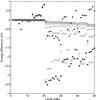 |
Fig. 1 Energy differences between our FAC calculations and the HFR1 results. The level energy differences are plotted versus the level index. Open squares: FAC6 minus FAC1. Open circles: FAC6 minus FAC2. Cross: FAC6 minus FAC3. Open diamonds: FAC6 minus FAC4. Open triangles: FAC6 minus FAC5. Solid circles: FAC6 minus HFR1 (Palmeri et al. 2008). Solid squares: FAC1 minus HFR1 (Palmeri et al. 2008). |
Experimental investigations of Si ix K-shell spectra are difficult in the laboratory. As stated in the introduction, no isolated lines of Si ix were observed using beam-foil methods (Trabert et al. 1979; 1982; Mosnier et al. 1986). The main reasons are that it is difficult to generate these K-vacancy states since the needed energies are usually higher than the ion ionization energy, and the high auto-ionization rates of these K-vacancy states depress the production of fluorescence yielding, thus these K-lines from Si ix are relatively very weak. The available experimental measurements by Faenov et al. (1994) are listed in Table 2. The largest wavelength difference between our FAC6 calculations and those of the experimental results is 8 mÅ, which is consistent with our former work on Si xi (Wei et al. 2010). Theoretical calculations from Palmeri et al. (2008) with the code HFR are also listed in Table 2, labeled HFR1. The wavelength differences between their results and those of the experimental measurements are lower than 10 mÅ, which is similar to our results. The theoretical results from Chen et al. (1997), based on a multiconfiguration Dirac-Fock (MCDF) method, are listed in Table 2. Relative larger wavelength differences, which can be as large as 35 mÅ, are found when comparing their results with those of the experimental measurements, which suggests that our works are more consistent with those of Palmeri et al. (2008).
Wavelengths of K-shell transitions in Si ix
It is also interesting to compare our results with those of the above theoretical calculations for all the transition wavelengths. The wavelength differences between our results (FAC1 and FAC6) and HFR1 (Palmeri et al. 2008) are shown in Fig. 2. The largest wavelength difference between FAC6 and HFR1 is lower than 13 mÅ, while the difference between FAC1 and HFR1 is lower than 8 mÅ. The average wavelength difference between FAC6 and HFR1 is 5 mű 2.9 mÅ, while it is 3 ± 2.4 mÅ between FAC1 and HFR1. The FAC6 wavelengths generally agree with HFR1, while the agreement between FAC1 and HFR1 is even better. This is because the CI effects from high-energy configurations have not been included in either the FAC1 or HFR1 calculations, as discussed above for energy levels. As shown in Fig. 2, large wavelength differences are found when comparing FAC6 with those from Chen et al. (1997). The largest wavelength difference is 37 mÅ and the average difference is 12 mÅ with a large standard deviation 13.8 mÅ. This big discrepancy is beyond the error ranges of our FAC6 or HFR1. Behar & Netzer (2002) have presented the strongest transition line for C-like Si ix is 6.939Å in wavelength, which also agrees well with our FAC6, and the difference is only 1 mÅ. By comparison with both experimental and previous theoretical results, we conclude that the wavelength of our FAC6 are with an accuracy about 15 mÅ.
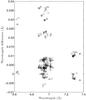 |
Fig. 2 Wavelength differences between our FAC calculations, HFR1 results, and the results from the MCDF method. The wavelength differences are plotted versus FAC6 wavelengths in Å for Si ix. Diamonds: FAC1 with HFR1 (Palmeri et al. 2008). Circles: FAC6 with HFR1 (Palmeri et al. 2008). Squares: FAC6 with MCDF method (Chen et al. 1997). |
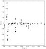 |
Fig. 3 Comparison of radiative rates between different FAC calculations. The ratio is plotted versus the FAC6 radiative rates. Squares: FAC6/FAC1. Circles: FAC6/FAC2. Cross: FAC6/FAC3. Diamond: FAC6/FAC4. Triangle: FAC6/FAC5. Solid dots are transitions originating from levels 34, 35, 38, and 39. |
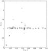 |
Fig. 4 Comparison of radiative rates between FAC6 and the results from HFR1 and FAC1. Squares: HFR1 (Palmeri et al. 2008). Circles: FAC1 (with radiative rates higher than 1E + 13(s-1)). |
3.2. Radiative rates
Before we tested the accuracy of our radiative rates, we investigated the CI effects from configurations of high-energy levels. Detailed comparison were carried out on the radiative rates between our FAC1, FAC2, FAC3, FAC4, FAC5, and FAC6 calculations. Only the ratios for the strong transition rates (>1E + 13s-1) are shown in Fig. 3. All transitions whose upper levels belongs to configurations 1s2s22p3 and 1s2p5, agree well within 5%, except for two transitions within 20%. This indicates that even if more configurations included, the CI effects on radiative rates can be neglected. These results agree with the findings of Hasoğlu et al. (2008). They used the multiconfiguration Breit-Pauli (MCBP) method to calculate radiative rates for 1s2s22p3 isoelectronic sequence, and found changes lower than 5% in radiative rates by including n = 3 configurations. However, large changes are found for transitions belonging to the configuration 1s2s2p4. In Fig. 3, the transition rates from levels 34, 35, 38, and 39, which belong to configuration 1s2s2p4, can change by as much as 75% between FAC1 and FAC6. These differences are gradually reduced to be lower than 5% with more extensive configurations included. Similarly to the energy levels, distinct changes occur in radiative rates when n = 3 configurations are taken into account in the calculations, since energy levels from both n = 2 and n = 3 configurations are very similar and CI effects are strong. Thus, our results show that the configurations from high-energy levels have strong CI effects on transitions from 1s2s2p4 configurations in Si ix and need to be included in atomic calculations.
To assess the accuracy of our FAC6 calculations, comparisons of our results with those from Palmeri et al. (2008) were carried out for the strong transitions (>1E + 13s-1). In our previous Be-like Si xi work, results calculated with the FAC code and those from Palmeri et al. (2008) agreed well for these strong transitions (within 10%). As shown in Fig. 4, for C-like Si ix, most radiative rates agree well with those from Palmeri et al. (2008), and the differences are lower than 10%. Large discrepancies exist both between FAC1 and HFR1 and between FAC6 and HFR1 for transitions originating from levels 34, 35, 38, and 39. The differences between FAC6 and HFR1 can be partly explained by the different configurations taken into account in the calculations, and the main reason for these differences is the relativistic effects. The levels 34 (1s(2S)2s2p4(4P) ) and 39 (1s(2S)2s2p4(2D)
 ) do not couple to each other in non-relativistic conditions. However, these two levels show strong relativistic interactions through spin-orbit interaction because of the same angular momentum J = 1 and the very similar energy values. Thus, the perturbation methods may not fully account for these relativistic effects. A similar explanation is valid for levels 35 (1s(2S)2s2p4(4P)
 ) and 38 (1s(2S)2s2p4(2D)
 ). For the weak transitions, as pointed out by Aggarwal et al. (2006), large differences commonly exist because of their sensitivities to the mixing coefficients. In total, 71% transitions have radiative rates within 20% between FAC6 and HFR1. By comparison with the radiative rates listed by Chen et al. (1997), we find large scatter even for the strong transitions, and most of them exceed 50%, which is not surprising since a good agreement is found between our FAC6 results with those from Palmeri et al. (2008). Inappropriate choice of the orbital wave function may be the reason for this discrepancy (Hasoğlu et al. 2008). In fact, we calculated the radiative rates with a purposely incorrect wave functions, and found a change of more than 20% in radiative rates.
3.3. Supplementary electronic tables
Two electronic tables are supplied at CDS as a supplement to this paper. In Table 3, state configurations, total angular quantum number, and parity of FAC6 are presented. In Table 4, the upper and lower level index are tabulated together with wavelengths, radiative rates, and absorption oscillator strengths.
Level energies of K-shell transitions for Si ix.
4. Summary and conclusions
We have calculated the energy levels, wavelengths, radiative rates, and oscillator strengths for the K-shell transitions of Si ix using the relativistic atomic code FAC (Gu 2003). The accuracy of the atomic data was assessed by detailed comparison with those of previous theoretical and experimental results. Our energy levels, wavelengths, and radiative rates are in generally closer to the results from Palmeri et al. (2008), while large differences in wavelengths and radiative rates were found when comparing our results with those from Chen et al. (1997). The large differences may be due to the inappropriate choice of the wave functions. Our energy levels are accurate to 3.5 eV and the wavelengths are accurate to within 15 mÅ. The radiative rates have an accuracy of 20% for most transitions. Our conclusions are supported from comparing our results with the compiled experimental level data from NIST. For the wavelengths, the differences with those of laser experimental measurements (Faenov et al. 1994) are lower than 8 mÅ. The large differences of radiative rates for some strong transitions, such as level 34 and 35, are mainly due to the strong spin-orbit interactions between these levels, which suggests that it is important to include relativistic effects in calculations.
The effects of CI from high-energy configurations were investigated. For 1s2s22p3 and 1s2p5 configurations of Si ix, this effect can be neglected, while for 1s2s2p4 configurations, significant changes are found, e.g. as large as 75% in radiative rates. We showed that including the configurations of high-energy levels, especially n = 3 configurations, is very important in Si ix K-shell data calculations.
K-shell transitions of Si ix
Acknowledgments
This work was supported by National Basic Research Program of China (973 Program) under grant 2013CBA01503 and the National Natural Science Foundation of China under grants Nos. 11103040, 11390371, 11173032, 11273032, 11273033, 11135012, and 11220101002.
References
- Aggarwal, K. M., Keenan, F. P., Kato, T., & Murakami, I. 2006, A&A, 460, 331 [NASA ADS] [CrossRef] [EDP Sciences] [Google Scholar]
- Andrade-Velázquez, M., Krongold, Y., Elvis, M., et al. 2010, ApJ, 711, 888 [NASA ADS] [CrossRef] [Google Scholar]
- Badnell, N. R. 1986, J. Phys. B, 19, 3827 [Google Scholar]
- Badnell, N. R. 1997, J. Phys. B, 30, 1 [Google Scholar]
- Bautista, M. A., Mendoza, C., Kallman, T. R., & Palmeri, P. 2003, A&A, 403, 339 [NASA ADS] [CrossRef] [EDP Sciences] [Google Scholar]
- Behar, E., & Netzer, H. 2002, ApJ, 570, 165 [NASA ADS] [CrossRef] [Google Scholar]
- Chang, Chulhoon, & Cui, Wei 2007, ApJ, 663, 1207 [NASA ADS] [CrossRef] [Google Scholar]
- Chen, M. H., Reed, K. J., McWilliams, D. M., et al. 1997, At. Data Nucl. Data Tables, 65, 289 [Google Scholar]
- Cowan, R. D. 1981, The Theory of Atomic Structure and Spectra Berkeley: Univ. California Press [Google Scholar]
- Dyall, K. G., Grant, I. P., Johnson, C. T., Parpia, F. A., & Plummer, E. P. 1989, Comput. Phys. Commun., 55, 424 [Google Scholar]
- Ebrero, J., Kaastra, J. S., Kriss, G. A., et al. 2013, MNRAS, 435, 3028 [NASA ADS] [CrossRef] [Google Scholar]
- Faenov, A. Ya., Pikuz, S. A., & Shlyaptseva, A. S. 1994, Phys. Scr., 49, 41 [NASA ADS] [CrossRef] [Google Scholar]
- Foster, A. R., & Testa, P. 2011, ApJ, 740, 52 [NASA ADS] [CrossRef] [Google Scholar]
- Gorczyca, T. W., Kodituwakku, C. N., Korista, et al. 2003, ApJ, 592, 636 [NASA ADS] [CrossRef] [Google Scholar]
- Gorczyca, T. W., Dumitriu, I., Hasoglu, M. F., et al. 2006, ApJ, 638, 121 [NASA ADS] [CrossRef] [Google Scholar]
- Güdel, M., & Naze, Y. 2009, A&ARv, 17, 309 [NASA ADS] [CrossRef] [Google Scholar]
- Gu, M. F., 2003, ApJ, 582, 1241 [NASA ADS] [CrossRef] [Google Scholar]
- Hell, N. 2012, Laboratory astrophysics: investigating the mystery of low charge states of Si and S in the HMXB Cyg X-1 Masters Thesis Dr Karl Remeis-Sternwarte, Universität Erlangen-Nürnberg [Google Scholar]
- Hell, N., Miškovičová, I., Brown, G. V., et al. 2013, Phys. Scr., 156, 014008 [NASA ADS] [CrossRef] [Google Scholar]
- Holczer, T., Behar, E., & Kaspi, S. 2007, ApJ, 663, 799 [NASA ADS] [CrossRef] [Google Scholar]
- Holczer, T., Behar, E., & Kaspi, S. 2010, ApJ, 708, 981 [NASA ADS] [CrossRef] [Google Scholar]
- Hasoğlu, M. F., Nikoli, D., Gorczyca, T. W., et al. 2008, Phy. Rev. A, 78, 2509 [NASA ADS] [CrossRef] [Google Scholar]
- Juett, A. M., & Chakrabarty, D. 2006, ApJ, 646, 493 [NASA ADS] [CrossRef] [Google Scholar]
- Kaastra, J. S., & Mewe, R. 1993, A&AS, 97, 443 [NASA ADS] [Google Scholar]
- Kallman, T. R., Bautista, M. A., Goriely, S., et al. 2009, ApJ, 701, 865 [NASA ADS] [CrossRef] [Google Scholar]
- Kaspi, S., Brandt, W. N., Netzer, H., et al. 2000, ApJ, 535, L17 [NASA ADS] [CrossRef] [PubMed] [Google Scholar]
- Kaspi, Shai, Brandt, W. N., Netzer, H., et al. 2001, ApJ, 554, 216 [NASA ADS] [CrossRef] [Google Scholar]
- Kaspi, S., Brandt, W. N., George, I. M., et al. 2002, ApJ, 574, 643 [NASA ADS] [CrossRef] [Google Scholar]
- King, A. L., Miller, J. M., & Raymond, J. 2012, ApJ, 746, 2 [NASA ADS] [CrossRef] [Google Scholar]
- Kramida, A., Ralchenko, Yu., Reader, J., and NIST ASD Team 2013, NIST Atomic Spectra Database (ver. 5.1), Available: http://physics.nist.gov/asd [2013, December 31], National Institute of Standards and Technology, Gaithersburg, MD [Google Scholar]
- Krongold, Y., Nicastro, F., Brickhouse, N. S., et al. 2003, ApJ, 597, 832 [NASA ADS] [CrossRef] [Google Scholar]
- Mosnier, J. P., Barchewitz, R., Senemaud, C., Cukier, M., & Dei-Cas, R. 1986 J. Phys. B: At. Mol. Opt. Phys., 19, 2531 [Google Scholar]
- Netzer, H., Kaspi, S., Behar, E., et al. 2003, ApJ, 599, 933 [NASA ADS] [CrossRef] [Google Scholar]
- Palmeri, P., Mendoza, C., Kallman, T. R., & Bautista, M. A. 2003, A&A, 403, 1175 [NASA ADS] [CrossRef] [EDP Sciences] [Google Scholar]
- Palmeri, P., Quinet, P., Mendoza, C., et al. 2008, ApJS, 177, 408 [NASA ADS] [CrossRef] [Google Scholar]
- Reeves, J. N., Porquet, D., Braito, V., et al. 2013, ApJ, 776, 99 [NASA ADS] [CrossRef] [Google Scholar]
- Sako, M., Kahn, S. M., Behar, E., et al., 2001, A&A, 365, L168 [NASA ADS] [CrossRef] [EDP Sciences] [Google Scholar]
- Safronova, U. I., & Urnov, A. M. 1979, J. Phys. B: At. Mol. Opt. Phys., 12, 3171 [NASA ADS] [CrossRef] [Google Scholar]
- Smith, M. A., Cohen, D. H., Gu, M. F., et al. 2004, ApJ, 600, 972 [NASA ADS] [CrossRef] [Google Scholar]
- Trabert, E., Armour, I. A., Bashkin, S., et al. 1979, J. Phys. B: At. Mol. Opt. Phys., 12, 1665 [NASA ADS] [CrossRef] [Google Scholar]
- Trabert, E., Fawcett, B. C., & Silver, J. D. 1982 J. Phys. B: At. Mol. Opt. Phys., 15, 3587 [Google Scholar]
- Vainshtein, L. A., & Safronova, U. I. 1978, At. Data Nucl. Data Tables, 21, 49 [Google Scholar]
- Vainshtein, L. A., & Safronova, U. I. 1980, At. Data Nucl. Data Tables, 25, 311 [Google Scholar]
- Verma, N., Jha, A. K. S., & Mohan, M. 2006, ApJS, 164, 297 [NASA ADS] [CrossRef] [Google Scholar]
- Wei, H. G., Shi, J. R., Zhao, G., et al. 2010, A&A, 522, A103 [NASA ADS] [CrossRef] [EDP Sciences] [Google Scholar]
- Young, A. J., Lee, J. C., Fabian, A. C., et al. 2005, ApJ, 631, 733 [NASA ADS] [CrossRef] [Google Scholar]
- Zeng, Jiaolong, & Yuan, Jianmin, 2006, Phy. Rev. E, 74, 5401 [Google Scholar]
All Tables
All Figures
|
Fig. 1 Energy differences between our FAC calculations and the HFR1 results. The level energy differences are plotted versus the level index. Open squares: FAC6 minus FAC1. Open circles: FAC6 minus FAC2. Cross: FAC6 minus FAC3. Open diamonds: FAC6 minus FAC4. Open triangles: FAC6 minus FAC5. Solid circles: FAC6 minus HFR1 (Palmeri et al. 2008). Solid squares: FAC1 minus HFR1 (Palmeri et al. 2008). |
| In the text | |
|
Fig. 2 Wavelength differences between our FAC calculations, HFR1 results, and the results from the MCDF method. The wavelength differences are plotted versus FAC6 wavelengths in Å for Si ix. Diamonds: FAC1 with HFR1 (Palmeri et al. 2008). Circles: FAC6 with HFR1 (Palmeri et al. 2008). Squares: FAC6 with MCDF method (Chen et al. 1997). |
| In the text | |
|
Fig. 3 Comparison of radiative rates between different FAC calculations. The ratio is plotted versus the FAC6 radiative rates. Squares: FAC6/FAC1. Circles: FAC6/FAC2. Cross: FAC6/FAC3. Diamond: FAC6/FAC4. Triangle: FAC6/FAC5. Solid dots are transitions originating from levels 34, 35, 38, and 39. |
| In the text | |
|
Fig. 4 Comparison of radiative rates between FAC6 and the results from HFR1 and FAC1. Squares: HFR1 (Palmeri et al. 2008). Circles: FAC1 (with radiative rates higher than 1E + 13(s-1)). |
| In the text | |
Current usage metrics show cumulative count of Article Views (full-text article views including HTML views, PDF and ePub downloads, according to the available data) and Abstracts Views on Vision4Press platform.
Data correspond to usage on the plateform after 2015. The current usage metrics is available 48-96 hours after online publication and is updated daily on week days.
Initial download of the metrics may take a while.