| Issue |
A&A
Volume 566, June 2014
|
|
|---|---|---|
| Article Number | A40 | |
| Number of page(s) | 9 | |
| Section | Galactic structure, stellar clusters and populations | |
| DOI | https://doi.org/10.1051/0004-6361/201423600 | |
| Published online | 05 June 2014 | |
Enhancement of magnetic fields arising from galactic encounters
1
School of Mathematics, University of Manchester,
Oxford Road,
Manchester,
M13 9PL,
UK
e-mail:
This email address is being protected from spambots. You need JavaScript enabled to view it.
2
Department of Physics, Moscow University,
119992
Moscow,
Russia
3
MPI für Radioastronomie, Auf dem Hügel 69,
53121
Bonn,
Germany
Received:
8
February
2014
Accepted:
2
April
2014
Abstract
Context. Galactic encounters are usually marked by a substantial increase in synchrotron emission of the interacting galaxies when compared with the typical emission from similar non-interacting galaxies. This increase is believed to be associated with an increase in the star formation rate and the turbulent magnetic fields resulting from the encounter, while the regular magnetic field is usually believed to decrease as a result of the encounter.
Aims. We attempt to verify these expectations.
Methods. We consider a simple, however rather realistic, mean-field galactic dynamo model where the effects of small-scale generation are represented by random injections of magnetic field resulting from star forming regions. We represent an encounter by the introduction of large-scale streaming velocities and by an increase in small-scale magnetic field injections. The latter describes the effect of an increase in the star formation rate caused by the encounter.
Results. We demonstrate that large-scale streaming, with associated deviations in the rotation curve, can result in an enhancement of the anisotropic turbulent (ordered) magnetic field strength, mainly along the azimuthal direction. This leads to a significant temporary increase of the total magnetic energy during the encounter; the representation of an increase in star formation rate has an additional strong effect. In contrast to expectations, the large-scale (regular) magnetic field structure is not significantly destroyed by the encounter. It may be somewhat weakened for a relatively short period, and its direction after the encounter may be reversed.
Conclusions. The encounter causes enhanced total and polarized emission without increase in the regular magnetic field strength. The increase in synchrotron emission caused by the large-scale streaming can be comparable to the effect of the increase in the star formation rate, depending on the choice of parameters. The effects of the encounter on the total magnetic field energy last only slightly longer than the duration of the encounter (ca. 1 Gyr). However, a long-lasting field reversal of the regular magnetic field may result.
Key words: galaxies: spiral / galaxies: magnetic fields / Galaxy: disk / magnetic fields / ISM: magnetic fields
© ESO, 2014
1. Introduction
Galactic encounters are spectacular phenomena that are usually marked by a substantial increase in synchrotron emission of the interacting galaxy when compared with the typical emission from similar non-interacting galaxies. The conventional interpretation associates this increase with an increase in the star formation rate (SFR) and in the strength of turbulent magnetic fields resulting from the encounter (Schleicher & Beck 2013). The radio-far infrared relation also holds for interacting galaxies (e.g. Ivison et al. 2010). The polarized radio emission, signature of compressed turbulent fields, is also known to be enhanced during the interaction (Vollmer et al. 2013). In contrast, the regular magnetic field, which is generated by the mean-field dynamo and contributes to the synchrotron radiation, is usually believed to decrease as a result of the encounter because the interaction disturbs one of the drivers of galactic dynamos, namely the rotation curve of the interacting galaxy. Of course, this naive expectation requires verification. In its full extent this would be a far from straightforward undertaking. Indeed, a detailed modelling of the process through an encounter would require modelling the magnetic fields and hydrodynamics of both galaxies as well as the interaction itself. This does not appear feasible in the near future. There is however a simplification which isolates the features of the interactions that appear salient for the evolution of the regular galactic magnetic field, and can allow its evolution to be followed through an encounter event, at least at an exploratory level.
Models for mean-field galactic dynamos have become increasingly more detailed (and so arguably more realistic). However, even with the very significant increase in computer resources that have become available over the last 20 years or so, severe approximations remain necessary. This is likely to remain true for the foreseeable future. Broadly speaking, models split into two groups. In one group, attempts are made to model in some detail processes in the interstellar medium (ISM), including cosmic ray transport and large-scale dynamics. Direct numerical simulation (DNS) in “boxes” can be used to provide estimates of transport coefficients (see e.g. Gressel et al. 2008; Brandenburg et al. 2008; Siejkowski et al. 2010). Models in the other group are in some ways less ambitious, using a simpler and more direct mean field formulation, often with rather ad hoc expressions for transport coefficients. Brandenburg (2014) gives an up-to-date review. Of course there is considerable overlap of these approaches, e.g. Hanasz et al. (2009). The latter type of model is much less demanding of computing resources, and readily allows extensive exploration of parameter space, and also the study of phenomena such as large-scale gas streaming in barred galaxies (e.g. Moss 1998; Moss et al. 1998, 2001, 2007; Kulpa-Dybel et al. 2011; Kim & Stone 2012), and the effects of spiral arms on dynamo action (Shukurov 1998; Moss 1998; Moss et al. 1998, 2013; Chamandy et al. 2013a,b). There are also many studies of the effects of externally driven gas flows on the gas content of galaxies (e.g. Vollmer et al. 2012 and references therein). Some of these also solve the passive induction equation, but do not include dynamo action, which is the main issue addressed in the current paper.
Our intention here is to revisit the effects of a galaxy-galaxy encounter, which generates large-scale non-circular velocities, on large-scale dynamo action in the larger galaxy. This problem seems to have been first studied by Moss et al. (1993) and Moss (1996). In the first of these papers, non-circular velocities taken from a dynamical model of the encounter between M 81 and its satellite NGC 3077 by Thomasson & Donner (1993) were introduced into a (necessarily) rather low-resolution and crude 3D dynamo model, and in the second a thin disc approximation was used. Moss et al. (1992) used a static velocity field corresponding to the instant of closest approach, whereas Moss (1997) used the fully time dependent velocity field. Although the dynamical model of the interaction is necessarily of low resolution by contemporary standards, we feel it is adequate to investigate some generic effects, and so we introduce the fully time dependent velocity field from Thomasson & Donner (1993) into the dynamo model recently proposed by Moss et al. (2012a,b). In this “hybrid” dynamo model, a crude representation of the effects of supernovae driven star formation regions in injecting smaller scale magnetic field into the ISM is included explicitly in a thin disc dynamo model. The resulting global magnetic fields display a number of novel features for mean field dynamos, including disorder on the scale of a kiloparsec or less, and small- and large-scale field reversals. We were particularly interested in seeing what additional effects might result, arising from the interaction of the non-circular velocities with the effects of the magnetic field injections. This sort of study has connections with cosmic ray driven dynamos of e.g. Siejkowski et al. (2014).
We first investigate the effects of the large-scale velocity field that is generated by the encounter, on the galactic magnetic field, and then tentatively explore the outcome of a parametrization of an associated increase in the star formation rate. A problem here is that the relation between the star formation rate and small-scale dynamo action is not completely resolved. We have not attempted any calibration of the novel effects with any standard model which quantifies the effect of an interaction on dynamo action via star formation, and simply represent this by a plausible parametrization. We stress that this point deserves further attention; however, such a study is obviously outside of the scope of this paper.
We describe our model in Sect. 2 including a brief recapitulation of the galactic dynamo model of Moss et al. (2012a,b). Our main result is that the interaction can significantly enhance synchrotron radiation emission, by its effects on both the small-scale and regular fields. Our detailed results are presented in Sect. 3 followed by discussion and conclusions in Sect. 4.
2. The model
2.1. The dynamo setup
The model is the thin disc model (”no-z” approximation) described in Moss et al. (2012a,b), with the addition of advection of magnetic field by the non-circular velocities. The model of Moss et al. (2012a,b) has the novel feature that small-scale field is continually injected at discrete locations, to simulate the effects of star forming regions in introducing small-scale field into the ISM. Briefly, we add random fields Binj = Binj0f(r,t) at n = 250 randomly chosen discrete locations with re-randomization (i.e. changing the location of the injection sites and the distribution of field strengths over them by choosing a new independent set of random numbers) at intervals dtinj ≈ 10 Myr. We note that the no-z approximation implicitly preserves the solenoidality condition ∇·B = 0 for both the dynamo generated and injected fields. Full details are given in Moss et al. (2012a,b). We take a flat disc, while noting that there is currently some uncertainty about whether galactic discs are substantially flat or flared (cf. Lazio & Cordes 1998); we note that further investigation of this point is needed, but it does not appear that our results are very sensitive to this assumption. Our approach is consistent with that of Thomasson & Donner (1993). The HI disc of the Milky Way does flare, but it is unclear whether the ionized gas disc does so, and the observational data for external galaxies are inconclusive. In most of the simulations to be discussed, we took the conventional alpha coefficient α and turbulent diffusivity η to be uniform throughout the disc; we intended a generic study with assumptions that were as simple as possible. We did run models with α(r) ∝ Ω(r) for comparison.
The code was implemented first on a Cartesian grid with 497 × 497 points, equally spaced, extended to just beyond the galactic radius, taken as R = 15 kpc. In this outer region beyond 15 kpc, there is no alpha-effect and the diffusivity retains its global value. This enables satisfactory treatment of the boundary conditions, see Moss et al. (2012a,b). This grid was used until the interaction began, a statistically steady state having been attained. The computational grid was extended further after the interaction began, to 617 × 617 points, with the same mesh size as before, allowing a larger exterior region to be included, see Sect. 2.4 below.
We use a nondimensional time unit, h2/η. With η = 1026 cm2 s-1 (used in all but one model presented) and h = 500 pc, this unit is approximately 0.78 Gyr. The timestep is fixed at approximately 0.04 Myr.
2.2. The velocity field
We adopted the velocity field for the interaction of M 81 and NGC 3077 of Thomasson & Donner (1993), with some minor modifications implemented for computational convenience. We took for the basic rotation curve the (purely axisymmetric and azimuthal) velocities from the dynamical model immediately before the interaction began. This had rather unsatisfactory behaviour near the galactic centre where the velocities remained approximately constant until very near the centre. Thus it was merged smoothly in the inner regions with a Brandt curve. At subsequent times through the interaction (which lasted about 0.9 Gyr), the non-circular velocities were as generated by the Thomasson & Donner code; the perturbations to the m = 0 azimuthal velocities at a given time were calculated by subtracting the raw m = 0 azimuthal velocities before the interaction from the current values. Fourier modes m = 1,2,3 were included from the Thomasson & Donner data. The interaction generates non-zero velocities for about 0.9 Gyr.
The salient models.
2.3. Choice of parameters
The large-scale velocities in the system are given (in km s-1) by the dynamical model, so once the values of the turbulent diffusivity and disc thickness are chosen, the conventional dynamo parameter Rω and the magnetic Reynolds number of the non-circular motions Rm are fixed. For reference, with η = 1026 cm s-1 and h = 500 pc, then Rω = 0.75, Rm = 1.5, and these values were used for the bulk of the simulations. For illustrative purposes we ran some models with other values of these parameters. The value of the parameter Rα is more uncertain: we took Rα = α0hη-1 = 1 as our standard value for the flat disc models. We note that we assume that α and η are uniform through the disc.
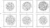 |
Fig. 1 Field vectors at times t ≈ 13.3,13.65,13.8 Gyr (row a)), and t ≈ 14.0,14.3,14.7 Gyr (row b)), for the canonical model 16. The interaction extends over the interval 13.3 ≤ t ≲ 14.2 Gyr. The vectors give the magnetic field direction, and their lengths are proportional to the magnetic field strengths. |
2.4. Extension of the model beyond the galactic radius
We found that when we set the boundary of the galactic disc at r = R = 15 kpc, which is the extent of the dynamical model and thus of the given velocities, then anomalous field gradients were generated near the boundary. For this reason we extended the velocities into the region r>R, reducing to very small values by r = 1.35R. This is certainly unphysical, in that we expect rotation curves to remain more-or-less flat until quite large radii. However, the interaction model does not provide data beyond r = R = 15 kpc, and this exterior region is only included to provide a satisfactory treatment of the outer parts of the disc; i.e. we do not try to represent accurately the region r>R. In r>R diffusion acts, but there is no alpha-effect. The dynamo model of Moss et al. (2012a,b) is already embedded in a surrounding passive region, so this is a minor modification which is found to give more satisfactory behaviour near r = R, and allows fields to be advected weakly beyond radius R.
2.5. Parametrization of the connection between the star formation rate and the dynamo governing parameters
In order to compare the effect of changes to the SFR caused by the interaction on the dynamo action we have to choose a parametrization of dynamo governing parameters which includes the star formation rate. Here we face the problem that such parametrization is little discussed in the current literature (see e.g. Mikhailov et al. 2012). However, this is an important problem which needs to be addressed separately. In order to make some progress we adopt a parametrization which looks at least plausible at first sight, i.e. we anticipate a simple quasi-linear relation between the SFR and the energy input into turbulence. This seems quite natural because a higher SFR means more supernovae and hence more energy input. As each supernova is a singular event, the energy input should simply add linearly. However, the question is whether the energy fractions going into turbulence, cosmic rays, and gas heating depend on the overall level of star formation or on the density of the surrounding medium. A higher SFR is expected in denser galaxies where the typical Mach numbers of supernova shocks should be higher. At the moment it remains unclear to what extent this affects the energy fractions. Additional uncertainties include whether a higher SFR is associated only with denser concentrations of SN, or larger star forming regions, or a combination. However, in any case it is to be expected that an increase in SFR will produce increased small-scale dynamo action. We represent this by an increase in the parameter Binj0, but could also consider increasing the size of the injection sites, or their number. Furthermore, we do not know the relation between energy deposited and the resulting small-scale dynamo field strength (see however Geng et al. 2012; Beck et al. 2012, which support the general view that something like equipartition will occcur).
We stress that the point deserves clarification; however, we restrict ourselves to this simple parametrization.
3. Results
3.1. The standard model
The more relevant models of those computed are summarized in Table 1.
We first discuss a model with the standard parameters described in Sect. 2.3, that is Rα = 1, Rω = 0.75, Rm = 1.5, f(r,t) = 1. Our computational procedure was to run the code until dimensionless time τ = 17, corresponding to an age of approximately 13 Gyr (“now”, cf. Moss et al. 2012a,b). As the field has long been settled into a statistically steady state by this time, the choice τ = 17 is not particularly significant in the current context and, for our purposes, it is the time from the start of the interaction at τ = 17 that is relevant. The non-circular velocities are then introduced, and the code is run for a further dimensionless time of about 4 units. As the interaction lasts for a little over 1 dimensionless time unit (ca 0.9 Gyr), by the time the simulation ends the field is found to approach a statistically steady state again. These models are basically similar to those of Moss et al. (2012a,b), except for the different rotation profile and larger galactic radius (here R = 15 kpc compared to 10 kpc).
In Fig. 1 we show snapshots of the magnetic field, from the beginning to just after the end of the interaction. We also show in Fig. 2 (solid curve) the time-averaged magnetic energy. (Time averages are used to smooth the instantaneous effects of the field injections, and are taken with a sliding window Δτ = 0.25, corresponding to physical time intervals of about 0.2 Gyr, except for Model 17 where Δτ = 0.50.)
To provide some orientation, we compare these results with a more conventional dynamo model (Model 9) with no field injections. This model has the same dynamo parameters as Model 16, and again was first run until time t ≈ 13.3 Gyr, by which time a steady state had long been established. At this time the interaction began, with the same underlying rotation curve as Model 16. Snapshots of the field configuration through and beyond the interaction are shown in Fig. 3. In slight contrast to Model 16 (see Fig. 1), in the last panel (t ≈ 14.7 Gyr) there are still small signs of the interaction process in r>R, but a steady state is reached by time 15.6 Gyr. Interestingly, the stable reversal present in the field before the interaction (first panel of Fig. 3) is absent from the post-interaction field, and the magnetic energy (shown in Fig. 4) does not return to its original value.
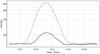 |
Fig. 2 Running time averages of total magnetic energy for Model 16 (solid) and Model 203 (broken). The interaction begins at t ≈ 13.3 Gyr and ends at t ≈ 14.2 Gyr. |
In both of these simulations, the effect of extending the velocity field beyond the nominal boundary of the galaxy at R = 15 kpc is visible, dragging the magnetic field into the exterior region. This is reminiscent of the extended field structures seen when modelling the effects of intergalactic “winds”, studied by Moss et al. (2012a,b). If the velocities in r>R are allowed to decrease more slowly with radius, then these “tails” extend farther in radius. Given the physical uncertainties associated with these regions, we did not pursue this point.
The value taken for the turbulent diffusivity, η = 1026 cm2 s-1, is conventional but uncertain. Thus, it is desirable to investigate the effects of changing the value of η (and so the magnetic Reynolds numbers). We found that the code could not handle the increase in Rω, Rm resulting from a decrease in η at an affordable resolution, but we show in Figs. 5 and 6 the results of increasing η to 2 × 1026 cm2 s-1. As the time unit scales with η-1, the values of τ for the panels of Fig. 5 differ substantially from those in the earlier figures, but the time intervals from the onset of the interaction are similar. The smaller value of Rω taken with an unchanged mean injected field strength means that fluctuations are larger in Model 17 than in Model 16. Also note that the local dynamo number is everywhere reduced by the increase in η.
3.2. A model with α(r) ∝ Ω(r)
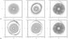 |
Fig. 3 Field vectors at dimensionless times t ≈ 13.3,13.65,13.8 Gyr (row a)), t = 14.0,14.3,14.7 Gyr (row b)), for the conventional Model 9 (without field injections) . The vectors give the magnetic field direction, and their lengths are proportional to the magnetic field strengths. |
In order to verify that our simple assumptions, in particular that α is constant throughout the disc, were not affecting the results significantly, we ran cases with α(r) ∝ Ω(r) (see e.g. Ruzmaikin et al. 1988). The value of Rα was now defined in terms of the central value α(0), and we ran several cases with the parameters of Model 16, but Rα > 1 (to compensate for the decrease in alpha with radius). We show in Fig. 7 the field configuration in mid-interaction at time t = 13.85 Gyr, and also the running time-averaged global energy, with Rα = 3. Comparison with the third panels of Figs. 1 and 2 suggests that there are few qualitative differences.
3.3. Dynamo action versus star formation in an encounter event
An enlargement of the total flux of synchrotron emission can also be connected with the well known increase in the SFR caused by an encounter. According to numerical simulations by Matteo et al. (2008), the increase in the SFR is by a factor smaller than 5 in about 85% of all major galaxy interactions and mergers for low redshift galaxies. To estimate the relative influence of the increase in SFR compared to that of the dynamo action and large-scale non-circular velocities alone, we performed the following experiments.
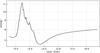 |
Fig. 4 Model 9, total magnetic energy. The interaction begins at t ≈ 13.3 Gyr. |
We took the basic Model 16, and in one case multiplied the field injection rate by the
factor  (1)between
times τbeg and τend, where
τbeg,τend
are the times of the start and finish of the interaction (i.e. when non-circular
velocities are non-zero). This model attempts to simulate a global increase in SFR, which
is increased by a factor of (1 +
qI) at mid-interaction. Perhaps not very
surprisingly, even with qI = 1 there is a marked increase (by a
factor of about 5) in the global magnetic energy at mid-interaction.
(1)between
times τbeg and τend, where
τbeg,τend
are the times of the start and finish of the interaction (i.e. when non-circular
velocities are non-zero). This model attempts to simulate a global increase in SFR, which
is increased by a factor of (1 +
qI) at mid-interaction. Perhaps not very
surprisingly, even with qI = 1 there is a marked increase (by a
factor of about 5) in the global magnetic energy at mid-interaction.
 |
Fig. 5 Field vectors at dimensionless times t ≈ 6.6,7.0,7.3 Gyr (row a)), t ≈ 7.5,7.8 Gyr (row b)), for Model 17 (with η = 2 × 1026 cm2 s-1). The vectors give the magnetic field direction, and their lengths are proportional to the magnetic field strengths. The interaction occurs during 6.6 ≤ t ≲ 7.5 Gyr. |
In the second case we set 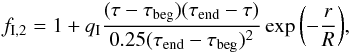 (2)simulating
an increase in SFR concentrated towards the central regions. Again, the global energy at
mid-interaction increases markedly compared to the standard case, Model 16 (but by less
than with fI,1 given by Eq.
(1) for the same qI = 1). Thus
the Models discussed above in Sects. 3.1 and 3.2 effectively take qI = 0.
(2)simulating
an increase in SFR concentrated towards the central regions. Again, the global energy at
mid-interaction increases markedly compared to the standard case, Model 16 (but by less
than with fI,1 given by Eq.
(1) for the same qI = 1). Thus
the Models discussed above in Sects. 3.1 and 3.2 effectively take qI = 0.
The plots of magnetic field vectors do not show marked differences to those displayed in Fig. 1, and so we do not show them.
We also ran cases with fI,2 given by Eq. (2) and qI = 2,10, with correspondingly larger increases in the global magnetic energy. The field vectors at t ≈ 13.85 Gyr with qI = 2,9 (Models 203, 204) are shown in Fig. 8.
3.4. Analysis of results
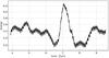 |
Fig. 6 Model 17, running time average of total magnetic energy. The interaction begins at t ≈ 6.6 Gyr and ends at t ≈ 7.5 Gyr. |
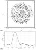 |
Fig. 7 Model 101 (with α ∝ Ω); a) field at t ≈ 13.85 Gyr, b) running time average of total magnetic energy. The interaction begins at t ≈ 13.3 Gyr and ends at t ≈ 14.2 Gyr. |
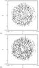 |
Fig. 8 Snapshots of field vectors at t ≈ 13.85 Gyr for a) Model 203, qi = 2; and b) Model 204, qI = 9. The scale factor for the vectors in b) is half that in a). |
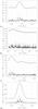 |
Fig. 9 Time averaged global Fourier integrals pi of
|
The effects of the interaction do not show up very dramatically in e.g. Fig. 1, but it is clear from Fig. 2 that there are profound effects on the magnetic field. This is in apparent contrast to the situation shown in Figs. 3 and 4. If the fields shown in Fig. 1 are averaged over a spatial scale larger than the scale of the injections, the confusing effects of the small-scale fields are removed, and a significant increase in the azimuthal magnetic field component by the non-circular velocities can be seen. However, this field is still turbulent anisotropic (i.e. ordered)1, but the regular large-scale field may be weakened (see Fig. 11a,b) as both azimuthal magnetic field directions can be found. These effects contribute strongly to the increase in global energy through the interaction, as seen in Fig. 2. Such an ordered field increases the total as well as the polarized emission. However, it can only partly be regarded as being part of the large-scale (regular) magnetic field of the disc.
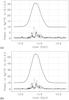 |
Fig. 10 Running time averages of global Fourier integrals pi of
|
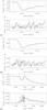 |
Fig. 11 Running time averages of global Fourier integrals Pi of Bφ through and beyond the interaction, (which begins at t ≈ 13.3 Gyr and ends at t ≈ 14.2 Gyr). Upper panelsP0, lower panelsP1 (continuous), P2 (broken), P3 (dotted): a) Model 16; b) Model 203; c) Model 9 (no field injections, data not averaged). |
In order to display this more clearly, we computed the global integrals of magnetic
energy in the azimuthal field  ,
,
 ,
m =
0,1,2,3,
n =
1,2,3 during the interaction. We
then set
,
m =
0,1,2,3,
n =
1,2,3 during the interaction. We
then set  ,
with g0 =
0. The results are shown in Fig. 9
for models 16 and 17 (with η =
1026 and 2 ×
1026 cm2 s-1, respectively), and also for Models 201 and 202. The
physical appearance of the fields (Figs. 1 and 5) and the time-averaged energies (Figs. 2 and 6) quite
rapidly approach their pre-interaction states after the interaction has ended. The effects
of the interaction are primarily seen in the mode m = 0, as are the gross
effects of the field injections, see the upper (continuous) curves in the panels of Fig.
9. Plausibly this is because the field injections
occur on a much shorter timescale than that of the interaction, and also the decay times
of the small-scale field components are relatively short. Furthermore their spatial scale
is smaller than that of the Fourier modes m = 0−3 analysed. We show in Fig. 10 the comparable plots for Models 202 and 203, where
the increase in energy in mode m = 0 can be seen when compared to that of Model 16
shown in Fig. 9a.
,
with g0 =
0. The results are shown in Fig. 9
for models 16 and 17 (with η =
1026 and 2 ×
1026 cm2 s-1, respectively), and also for Models 201 and 202. The
physical appearance of the fields (Figs. 1 and 5) and the time-averaged energies (Figs. 2 and 6) quite
rapidly approach their pre-interaction states after the interaction has ended. The effects
of the interaction are primarily seen in the mode m = 0, as are the gross
effects of the field injections, see the upper (continuous) curves in the panels of Fig.
9. Plausibly this is because the field injections
occur on a much shorter timescale than that of the interaction, and also the decay times
of the small-scale field components are relatively short. Furthermore their spatial scale
is smaller than that of the Fourier modes m = 0−3 analysed. We show in Fig. 10 the comparable plots for Models 202 and 203, where
the increase in energy in mode m = 0 can be seen when compared to that of Model 16
shown in Fig. 9a.
In order to isolate more clearly the effects of the interaction on the global scale
field, we evaluated integrals Fm,Gn,
and quantities Pi analogous to the
fm,gn,pi
defined above, with  replaced by
the signed quantity Bφ in the integrals.
The integrals
replaced by
the signed quantity Bφ in the integrals.
The integrals  and
and
 are a measure of the regular
(mean) field. The results for Models 16 and 203 are shown in Fig. 11, together with those for Model 9 (no field injections). Now there is
almost no increase in the magnitude of the quantities P0 during the
interaction, and the magnitudes of P1,P2,P3
are comparable. However, there is a long-lived change of sign of P0, apparently
corresponding to the reversals that are discernable in the field vector plots, and the
values of P0 do not quickly revert to their
pre-interaction levels (i.e. there is a long term effect on the large-scale field). In
effect, the interaction resets the initial state for the post-interaction evolution. It is
known (e.g. Moss & Sokoloff 2013), that in
a non-linear dynamo model different initial conditions can produce different stable
states, with or without field reversals, if the system is initially non-linear. This is in
marked contrast to the situation shown in Figs. 9 and
10, where p0 quickly
returns to the pre-interaction state. It may be relevant that in Model 9 (with no field
injections) there is a long-term change in the global field structure. The corresponding
behaviour of the Fourier modes for this model is shown in Fig. 11c. The change in power in the mode m = 0 seems to correspond
to the removal of the field reversal in the post interaction state. The higher modes are
then decaying.
are a measure of the regular
(mean) field. The results for Models 16 and 203 are shown in Fig. 11, together with those for Model 9 (no field injections). Now there is
almost no increase in the magnitude of the quantities P0 during the
interaction, and the magnitudes of P1,P2,P3
are comparable. However, there is a long-lived change of sign of P0, apparently
corresponding to the reversals that are discernable in the field vector plots, and the
values of P0 do not quickly revert to their
pre-interaction levels (i.e. there is a long term effect on the large-scale field). In
effect, the interaction resets the initial state for the post-interaction evolution. It is
known (e.g. Moss & Sokoloff 2013), that in
a non-linear dynamo model different initial conditions can produce different stable
states, with or without field reversals, if the system is initially non-linear. This is in
marked contrast to the situation shown in Figs. 9 and
10, where p0 quickly
returns to the pre-interaction state. It may be relevant that in Model 9 (with no field
injections) there is a long-term change in the global field structure. The corresponding
behaviour of the Fourier modes for this model is shown in Fig. 11c. The change in power in the mode m = 0 seems to correspond
to the removal of the field reversal in the post interaction state. The higher modes are
then decaying.
4. Discussion
Both the interaction itself and any increase in SFR associated with the interaction can increase the overall magnetic energy, due to the effects of injected random fields and their subsequent shearing, that give rise to unpolarized and polarized synchrotron radiation, respectively. In more detail, our results do not seem particularly sensitive to the chosen radial distribution of the enhancement of the SFR, as shown by our experiments with the enhancement function f(r,t) given by Eqs. (1) and (2 with qI = 1). The maximum enhancement of energy is positively correlated with qI. Observed increases in SFR during encounters are rarely greater than by a factor of 5 (e.g. Matteo et al. 2008), but it is important to remember that our parameter qI is only a proxy for the effects of enhanced SFR on small-scale dynamo action. We note again that any assumed linear relation between qI and SFR is only a crude plausible approximation. It is quite probable that for high SFR the effects of the individual supernovae explosions can no longer be considered as independent, and the relation begins to saturate. We use the parameter Binj0 as a proxy for all these possibilities. We cannot address this issue here; clearly the problem deserves specific investigation (e.g. Geng et al. 2012; Beck et al. 2012). We note that our results are broadly consistent with studies of cosmic ray driven dynamos (e.g. Siejkowski et al. 2014, and references therein). These studies find that for, modest values of the SFR, galactic fields are enhanced, but that the dynamo ceases to operate for very high values of SFR.
If we look at the field vector plots during the interaction, even with large values of
Binj some large-scale order appears visible,
generated by the effects of large-scale velocity shear (especially differential rotation on
the injected field, see e.g. Fig. 8). In these models
the magnitude of  in the lower modes (here
concentrated in m =
0, see Fig. 9) will be a measure of
anisotropic fields and will determine the level of polarized intensity when observing at a
low spatial resolution.
in the lower modes (here
concentrated in m =
0, see Fig. 9) will be a measure of
anisotropic fields and will determine the level of polarized intensity when observing at a
low spatial resolution.
5. Conclusions
Overall we can conclude that an interaction affects the magnetic field configuration. The effects on the field can take the form of additional reversals of the large-scale magnetic field, can lead to a concentration of magnetic fields in rings, and so on. The limiting point, however, is that we only have snapshots of magnetic field configurations for a few examples, so it is problematic to isolate effects of interactions in the evolution of galactic magnetic field configurations; we can play with the governing galactic dynamo parameters to obtain configurations which more-or-less resemble fields observed in any particular case. We note again that we have used an old, low-resolution, dynamical model, so our results can only be regarded as generic.
A reasonable way to isolate the effects of interactions observationally would be by a statistical study of interacting and non-interacting galaxies. The immediate feature of interest in our results is the peak in global energy in the epoch of encounter. The total magnetic energy increases during an encounter by 15%, 80%, 250% for Models 17, 101 and 202 respectively, which should lead to a corresponding increase in the total flux of synchrotron radiation.
I.e. appearing ordered in radio polarization observations.
Acknowledgments
D.S. is grateful for financial support from RFBR under grant 12-02-00170-a and to MPIFR for hospitality. The velocity data was provided by Magnus Thomasson. The referee, Prof. K. Otmianowski-Mazur, is thanked for her careful comments.
References
- Beck, A. M., Lesch, H., Dolag, K., et al. 2012, MNRAS, 422, 2152 [NASA ADS] [CrossRef] [Google Scholar]
- Brandenburg, A. 2014 [arXiv:1402.0212] [Google Scholar]
- Brandenburg, A., Rädler, K.-H., & Schrinner, M. 2008, A&A, 482, 739 [NASA ADS] [CrossRef] [EDP Sciences] [Google Scholar]
- Chamandy, L., Subramanian, K., & Shukurov, A. 2013a, MNRAS, 428, 3569 [NASA ADS] [CrossRef] [Google Scholar]
- Chamandy, L., Subramanian, K., & Shukurov, A. 2013b, MNRAS, 433, 3274 [NASA ADS] [CrossRef] [Google Scholar]
- Geng, A., Kotarba, H., Bürzle, F., et al. 2012, MNRAS, 419, 3571 [NASA ADS] [CrossRef] [Google Scholar]
- Gressel, O., Elstner, D., Ziegler, U., & Rüdiger, G. 2008, A&A, 486, L35 [NASA ADS] [CrossRef] [EDP Sciences] [Google Scholar]
- Hanasz, M., Woltanski, D., & Kowalik, K. 2009, ApJ, 706, 155 [Google Scholar]
- Ivison, R. J., Magnelli, B., Ibar, E., et al. 2010, A&A, 518, L31 [NASA ADS] [CrossRef] [EDP Sciences] [Google Scholar]
- Kim, W.-T., & Stone, J. M. 2012, ApJ, 751, 21 [NASA ADS] [CrossRef] [Google Scholar]
- Kulpa-Dybel, K., Otmianowska-Mazur, K., Kulesza-Åydzik, B., et al. 2011, ApJ, 733, L18 [NASA ADS] [CrossRef] [Google Scholar]
- Lazio, T. J. W., Cordes, J. M. 1998, in Radio Emission from Galactic and Extragalactic Compact Sources, eds. J. A. Zensus, G. B.Taylor, & J. M. Wrobel, IAU Colloq., 164, 329 [Google Scholar]
- Matteo, P. D., Combes, F., Melchior, A. L., & Semelin, B. 2008, ASP Conf. Ser., 390, 178 [NASA ADS] [Google Scholar]
- Mikhailov, E. A., Sokoloff, D. D., & Efremov, Yu. N. 2012, Astron. Lett., 38, 543 [NASA ADS] [CrossRef] [Google Scholar]
- Moss, D. 1996, A&A, 315, 63 [NASA ADS] [Google Scholar]
- Moss, D. 1997, MNRAS, 289, 554 [NASA ADS] [CrossRef] [Google Scholar]
- Moss, D. 1998, MNRAS, 297, 860 [NASA ADS] [CrossRef] [Google Scholar]
- Moss, D., & Sokoloff, D. 2013, Geophys. Astrophys. Fluid. Dyn. 107, 49 [Google Scholar]
- Moss, D., Korpi, M., Rautiainen, P., & Salo, H. 1998, A&A, 329, 895 [NASA ADS] [Google Scholar]
- Moss, D., Brandenburg, A., Donner, K. J., & Thomasson, M. 1993, ApJ, 409, 179 [NASA ADS] [CrossRef] [Google Scholar]
- Moss, D., Shukurov, A., Sokoloff, D., Beck, R., & Fletcher, A. 2001, A&A, 380, 55 [NASA ADS] [CrossRef] [EDP Sciences] [Google Scholar]
- Moss, D., Snodin, A. P., Englmaier, P., et al. 2007, A&A, 465, 157 [NASA ADS] [CrossRef] [EDP Sciences] [Google Scholar]
- Moss, D., Stepanov, R., Arshakian, T. G., et al. 2012a, A&A, 537, A68 [NASA ADS] [CrossRef] [EDP Sciences] [Google Scholar]
- Moss, D., Sokoloff, D., & Beck, R. 2012b, A&A, 544, A5 [Google Scholar]
- Moss, D., Beck, R., Sokoloff, D., et al. 2013, A&A, 556, A147 [NASA ADS] [CrossRef] [EDP Sciences] [Google Scholar]
- Ruzmaikin, A. A., Shukurov, A. M., & Sokoloff, D. D. 1988, Magnetic Fields of Galaxies (Dordrecht: Kluwer) [Google Scholar]
- Schleicher, D. R. G., & Beck, R. 2013, A&A, 556, A142 [NASA ADS] [CrossRef] [EDP Sciences] [Google Scholar]
- Shukurov, A. 1998, MNRAS, 299, L21 [NASA ADS] [CrossRef] [Google Scholar]
- Siejkowski, H., Soida, M., Otmianowska-Mazur, K., Hanasz, M., & Bomans, D. J. 2010, A&A, 510, 97 [Google Scholar]
- Siejkowski, H., Otmianowska-Mazur, K., Soida, M., Bomans, D. J., & Hanasz, M. 2014, A&A, 526, 136 [Google Scholar]
- Thomasson, M., & Donner, K. J. 1993, A&A, 272, 153 [NASA ADS] [Google Scholar]
- Vollmer, B., Bane, J., & Soida, M. 2012, A&A, 547, A39 [NASA ADS] [CrossRef] [EDP Sciences] [Google Scholar]
- Vollmer, B., Soida, M., Beck, R., et al. 2013, A&A, 553, A116 [NASA ADS] [CrossRef] [EDP Sciences] [Google Scholar]
All Tables
All Figures
|
Fig. 1 Field vectors at times t ≈ 13.3,13.65,13.8 Gyr (row a)), and t ≈ 14.0,14.3,14.7 Gyr (row b)), for the canonical model 16. The interaction extends over the interval 13.3 ≤ t ≲ 14.2 Gyr. The vectors give the magnetic field direction, and their lengths are proportional to the magnetic field strengths. |
| In the text | |
|
Fig. 2 Running time averages of total magnetic energy for Model 16 (solid) and Model 203 (broken). The interaction begins at t ≈ 13.3 Gyr and ends at t ≈ 14.2 Gyr. |
| In the text | |
|
Fig. 3 Field vectors at dimensionless times t ≈ 13.3,13.65,13.8 Gyr (row a)), t = 14.0,14.3,14.7 Gyr (row b)), for the conventional Model 9 (without field injections) . The vectors give the magnetic field direction, and their lengths are proportional to the magnetic field strengths. |
| In the text | |
|
Fig. 4 Model 9, total magnetic energy. The interaction begins at t ≈ 13.3 Gyr. |
| In the text | |
|
Fig. 5 Field vectors at dimensionless times t ≈ 6.6,7.0,7.3 Gyr (row a)), t ≈ 7.5,7.8 Gyr (row b)), for Model 17 (with η = 2 × 1026 cm2 s-1). The vectors give the magnetic field direction, and their lengths are proportional to the magnetic field strengths. The interaction occurs during 6.6 ≤ t ≲ 7.5 Gyr. |
| In the text | |
|
Fig. 6 Model 17, running time average of total magnetic energy. The interaction begins at t ≈ 6.6 Gyr and ends at t ≈ 7.5 Gyr. |
| In the text | |
|
Fig. 7 Model 101 (with α ∝ Ω); a) field at t ≈ 13.85 Gyr, b) running time average of total magnetic energy. The interaction begins at t ≈ 13.3 Gyr and ends at t ≈ 14.2 Gyr. |
| In the text | |
|
Fig. 8 Snapshots of field vectors at t ≈ 13.85 Gyr for a) Model 203, qi = 2; and b) Model 204, qI = 9. The scale factor for the vectors in b) is half that in a). |
| In the text | |
|
Fig. 9 Time averaged global Fourier integrals pi of
|
| In the text | |
|
Fig. 10 Running time averages of global Fourier integrals pi of
|
| In the text | |
|
Fig. 11 Running time averages of global Fourier integrals Pi of Bφ through and beyond the interaction, (which begins at t ≈ 13.3 Gyr and ends at t ≈ 14.2 Gyr). Upper panelsP0, lower panelsP1 (continuous), P2 (broken), P3 (dotted): a) Model 16; b) Model 203; c) Model 9 (no field injections, data not averaged). |
| In the text | |
Current usage metrics show cumulative count of Article Views (full-text article views including HTML views, PDF and ePub downloads, according to the available data) and Abstracts Views on Vision4Press platform.
Data correspond to usage on the plateform after 2015. The current usage metrics is available 48-96 hours after online publication and is updated daily on week days.
Initial download of the metrics may take a while.